1 Introduction

One important property of field theories with spontaneous symmetry breaking is that the life-time of energetically meta-stable vacuum states can be very long. This can lead to the partitioning of the universe into regions of different meta-stable vacuum states. One of these structures is called cosmic strings [1]. Such kind of structures represent thin tubes of false vacuum and are expected to be of large linear mass density $\mu$ and can also carry intrinsic angular momentum $J$.

The cosmic strings affect the spacetime mainly topologically, giving a conical structure to the space region around the cone of the string. The conical topology may be responsible for several gravitational effects, gravitational lensing [2] and particle production due to the changing gravitational field during the formation of such object [3] being some examples.

There is a lot of papers studying quantum processes in a cosmic string spacetime. Of special interest to us are the following: [4] where pair production in a straight cosmic string spacetime is discussed, [5] where the response function of detectors in the presence of the cosmic strings is calculated, and [6] where the spinning cosmic string spacetime is investigated. Finally spinning cosmic strings were studied also by Gal’tsov et al. and also Letelier. These authors investigated chiral strings generating a chiral conical spacetime [7].

In this paper we are interested in two calculations. First, to analyse the energy momentum distribution of a time dependente spinning cosmic string spacetime. Second, to estimate the particle production due to the changing gravitational field in the situation of gradual loss of angular momentum.

2 General spinning cosmic string spacetimes

The Einstein’s gravity equation of general relativity is given by:

$$G_{\mu\nu}=-\kappa T_{\mu\nu}$$ (1)

where the constant $\kappa$ is defined to give the correct Newtonian limit, resulting in

$$\kappa=\frac{8\pi G}{c^{4}}.$$ (2)

$G$ and $c$ appearing in the latter equation represent the Newtonian gravitational constant and light velocity, respectively.

In order to obtain the geometry generated by a rotating cosmic string we proceed in the following way. First, we choose a cylindrical coordinate system ($x^{\mu}:\{ct,r,\varphi,z\}$) in which an infinitely long and thin cosmic string lies along the $z$-axis. We consider a stationary string carrying linear densities of mass $\mu$ and angular momentum ${\cal J}_{\scriptscriptstyle 0}$. The mass density is proportional to a two-dimensional delta function ($\delta$-function) while the angular momentum density is proportional to the derivatives of $\delta$-functions. The $T_{\scriptscriptstyle 00}$ and $T_{\scriptscriptstyle 0i}$ components of the associated energy momentum tensor will be proportional to $\delta$-function and its derivatives, respectively. Thus, Einstein equations leads to the geometry

$$[g_{\mu\nu}]=\left(\begin{array}[]{cccc}c^{2}&0&4G{\cal J}_{\scriptscriptstyle 0}/c^{2}&0\\ 0&-1&0&0\\ 4G{\cal J}_{\scriptscriptstyle 0}/c^{2}&0&-\left(b^{2}r^{2}-16G^{2}{\cal J}_{\scriptscriptstyle 0}^{2}/c^{6}\right)&0\\ 0&0&0&-1\end{array}\right)$$ (3)

with

$$b\equiv 1-\frac{4G\mu}{c^{2}}.$$ (4)

From these metric components we can construct the associated line element

$$ds^{2}=\left(cdt+\frac{4G{\cal J}_{\scriptscriptstyle 0}}{c^{3}}d\varphi\right)^{2}-dr^{2}-b^{2}r^{2}d\varphi^{2}-dz^{2}.$$ (5)

Therefore, as was noticed by Deser and Jackiw [8], the two-parameter $(\mu;{\cal J}_{\scriptscriptstyle 0})$ metric tensor showed in equation (3) represents the general time-independent solution to gravitational Einstein equations outside any matter distribution lying in a bounded region on the plane and having cylindrical symmetry. In this work we will consider only the exterior region of the cosmic string. Thus the $\delta$-functions will be suppressed in our analysis of the energy momentum tensor generating a spacetime configuration due to a cosmic string loosing angular momentum.

In the same way the exact spacetime metric representing the vacuum solution of a static cylindrically symmetric cosmic string is found [9] to be

$$ds^{2}=c^{2}dt^{2}-dr^{2}-b^{2}r^{2}d\varphi^{2}-dz^{2}.$$ (6)

Obviously this metric is a particular case of the former, equation (5), with null density of angular momentum.

Thus it arises the questions: How can we go from a spinning cosmic string spacetime to a static one and what is the rate of particle production between these two asymptotic limits?

First of all, let us assume that the cosmic string is generated in such way that there is spontaneous loss of energy associated with change in its rotation velocity, i.e., loss of density of angular momentum. Quantitatively such process would correspond to a non-stationary spacetime geometry that could be described by the metric (5) with ${\cal J}_{\scriptscriptstyle 0}$ replaced by a general function of time ${\cal J}(t)$:

$$ds^{2}=\left[cdt+\frac{4G{\cal J}(t)}{c^{3}}d\varphi\right]^{2}-dr^{2}-b^{2}r^{2}d\varphi^{2}-dz^{2}$$ (7)

and provided with the asymptotic conditions

$$\lim_{t\rightarrow-\infty}{\cal J}(t) = {\cal J}_{\scriptscriptstyle 0}$$ (8)

$$\lim_{t\rightarrow+\infty}{\cal J}(t) = 0.$$ (9)

A specific choice for the density of angular momentum that solves the above relations is given by

$${\cal J}(t)=\frac{{\cal J}_{\scriptscriptstyle 0}}{2}\left[1-\tanh(t)\right].$$ (10)

In the following section we will look for the kind of matter content that generates such spacetime geometry.

3 Energy momentum distribution

As we can notice, the region between the two asymptotic limits represents a curved spacetime. From Einstein equations we show that the fluid configuration characterizing such geometry is represented by the following energy momentum tensor components

$$[T_{\mu\nu}]=-\frac{2G{\cal J}_{\scriptscriptstyle 0}}{\kappa r\cosh t}\left(\begin{array}[]{cccc}0&0&0&0\\ 0&\frac{2GJ_{\scriptscriptstyle 0}}{b^{2}r}F(t)&1&0\\ 0&1&0&0\\ 0&0&0&\frac{2GJ_{\scriptscriptstyle 0}}{b^{2}r}F(t)\end{array}\right)$$ (11)

with $F(t)$ defined by:

$$F(t)\equiv\frac{3+\sinh(2t)-2\cosh^{2}(t)}{\cosh^{3}(t)}.$$ (12)

Let us now analyze the properties of the above characterized fluid. First of all we define a 4-velocity vector field $V^{\mu}$

$$V^{\mu}=\delta^{\mu}_{0}$$ (13)

and the projector tensor $h_{\alpha\beta}$

$$h_{\alpha\beta}=g_{\alpha\beta}-V_{\alpha}V_{\beta}.$$ (14)

In the standard way, we express the energy momentum tensor in terms of its irreducible parts as

$$T_{\mu\nu}=(\rho+p)V_{\mu}V_{\nu}-pg_{\mu\nu}+q_{(\mu}V_{\nu)}+\Pi_{\mu\nu}$$ (15)

where we introduced the quantities related with the fluid, i.e., energy density, isotropic pressure, heat flux and anisotropic pressure, defined respectively as

$$\rho = T_{\mu\nu}V^{\mu}V^{\nu}$$ (16)

$$p = -\frac{1}{3}T_{\mu\nu}h^{\mu\nu}$$ (17)

$$q_{\alpha} = T_{\mu\nu}V^{\nu}h^{\mu}\mbox{}_{\alpha}$$ (18)

$$\Pi_{\mu\nu} = T_{\alpha\beta}h^{\alpha}\mbox{}_{\mu}h^{\beta}\mbox{}_{\nu}+ph_{\mu\nu}.$$ (19)

For the case we are analyzing here only isotropic and anisotropic pressure survive, and they result in:

$$p(t,r)=-\frac{8G^{2}J_{\scriptscriptstyle 0}^{2}}{3\kappa b^{2}c^{8}r^{2}}\left(\tanh^{2}t-1\right)\left(3\tanh^{2}t-2\tanh t-1\right)$$ (20)

and

$$[\Pi_{\mu\nu}]=-\frac{p(t,r)}{2}\left(\begin{array}[]{cccc}0&0&0&0\\ 0&1&\tilde{\pi}&0\\ 0&\tilde{\pi}&-2&0\\ 0&0&0&1\end{array}\right)$$ (21)

where

$$\tilde{\pi}\equiv-\frac{3b^{2}c^{4}r}{2GJ_{\scriptscriptstyle 0}}\left(\frac{1}{3\tanh^{2}t-2\tanh t-1}\right).$$ (22)

From what we have seen, outside the core of the string there is not energy density of matter but only flux of energy, that appears as pressure. From the Einstein equations we obtain the relation between the trace of the energy momentum tensor and the curvature of the spacetime ($R=\kappa T$), that results in:

$$R=-3\kappa p(t,r).$$ (23)

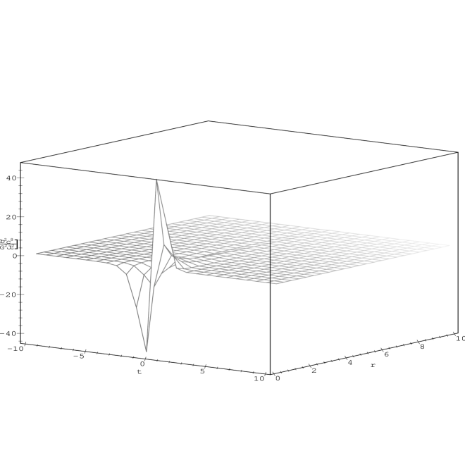
Figure 1: The spacetime curvature $R$ (as function of coordinates $t$ and $r$) generated by a spinning cosmic string loosing angular momentum during the time evolution.

The geometry of the spacetime is flat in the asymptotic regions corresponding to infinite past and infinite future. Therefore it is worth to analyze the behavior of the curvature in the intermediate region. In the figure 1 we plot the curvature $R$ as function of time $t$ and radial coordinate $r$ (distance from the $z$ axes of the string). For $t<<0$ the spacetime is approximately flat for all values of $r$, and for large values of $r$ it will still be flat for all values of $t$, as we would expect. As time $t$ goes from negative to positive values the curvature decreases until it reaches a minimum value at $t\approx-0.926$. After this point it begins to increase, becomes positive and reaches a maximum value at $t\approx 0.233$. Finally it asymptotically goes to zero. The two asymptotic spacetimes are flat. The only difference between them is that for $t\rightarrow-\infty$ the string is spinning with constant density of angular momentum $J_{\scriptscriptstyle 0}$.

As a general result of this analysis we obtained that the loss of angular momentum by a cosmic string causes a change in the metric properties of the spacetime. But changes in the gravitational field generate particles [10]. Thus we have to investigate the creation of particles and radiation by the changing gravitational field during the loss of angular momentum of a initially spinning cosmic string. We will treat this problem by performing the calculation of the Bogoliubov transformation entailed by this process.

4 Particle production between the asymptotic spacetimes

From the general geometry (7) and the conditions (8) and (9), in the two asymptotic regions — the infinite past and infinite future — the spacetime metric structures reduce to:

$$ds^{2}_{-\infty} = \left(dt+4GJ_{\scriptscriptstyle 0}d\varphi\right)^{2}-dr^{2}-b^{2}r^{2}d\varphi^{2}-dz^{2}$$ (24)

$$ds^{2}_{+\infty} = dt^{2}-dr^{2}-b^{2}r^{2}d\varphi^{2}-dz^{2}.$$ (25)

The above metrics represent the structure of the spacetime in the exterior region of a rotating and a non-rotating cosmic string, respectively.

In this section we will analyze the rate of particle production by the changing gravitational field between the two asymptotic spacetimes during the evolution of a cosmic string that looses angular momentum. A similar idea was used by Bernard and Duncan [11] to study a two dimensional Robertson-Walker model where the conformal scale factor has the same functional form as equation (10). In the two asymptotic limits, the spacetime becomes Minkowskian, and they obtained the mode solutions of the Klein-Gordon equation in these two limits. A straightforward calculation of the Bogoliubov coefficients between the in and out modes gives the rate of particle production during the expansion of the universe. It is worth to notice that such method was first introduced by L. Parker [12] in order to calculate particle creation by the expansion of the universe.

Let us consider a massive minimally coupled Hermitian scalar field $\phi(t,r,\varphi,z)$ defined at all points of the spacetime (7). The Klein-Gordon equation is given by:

$$\left[g^{\mu\nu}D_{\mu}D_{\nu}+M^{2}\right]\phi(t,r,\varphi,z)=0$$ (26)

where the symbol $D_{\alpha}$ represents the covariant derivative with respect to the metric $g_{\alpha\beta}$, and $M$ is the mass of the scalar field.

To maintain the energy produced in a limited region of the space we impose Dirichlet boundary conditions at $r=R$,

$$\left.\phi(t,r,\varphi,z)\right|_{r=R}=0$$ (27)

and periodic boundary conditions in $z$ with period $L$.

In order to circumvent the problem of the generation of closed time-like curves (CTC), we impose an additional vanishing boundary condition at $r=R_{0}>4GJ/b$. Thus, the radial coordinate has the domain $R_{0}<r<R$. For a careful study on how to construct quantum field theory in a spacetime with CTC, see for instance [13]. The same problem appears in $(2+1)$ dimensional gravity since the spinning cosmic string spacetime is exactly the solution of $(2+1)$ Einstein equations of a spinning point source [14].

The Klein-Gordon equation for the initial spacetime (24) reduces to the form:

$$\left[\left(1-\frac{16G^{2}J_{\scriptscriptstyle 0}^{2}}{b^{2}r^{2}}\right)\frac{\partial^{2}}{\partial t^{2}}-\frac{1}{r}\frac{\partial}{\partial r}\left(r\frac{\partial}{\partial r}\right)-\frac{1}{b^{2}r^{2}}\frac{\partial^{2}}{\partial\varphi^{2}}-\frac{\partial^{2}}{\partial z^{2}}+\frac{8GJ^{2}_{\scriptscriptstyle 0}}{b^{2}r^{2}}\frac{\partial^{2}}{\partial t\partial\varphi}+M^{2}\right]\phi(t,r,\varphi,z)=0.$$ (28)

The mode solutions $u_{j}$ are found to be

$$u_{j}(t,\vec{x})=N_{1}\,e^{-i\omega_{l}t}e^{ikz}e^{im\varphi}\left[\frac{J_{\mu}(qr)}{J_{\mu}(qR)}-\frac{Y_{\mu}(qr)}{Y_{\mu}(qR)}\right]$$ (29)

with

$$\mu \equiv \frac{|m+4GJ\omega_{l}|}{b}$$ (30)

$$q = \sqrt{\omega_{l}^{2}-k^{2}-M^{2}}$$ (31)

and

$$k=\frac{2\pi n}{L}.$$ (32)

In the above, $m,n=0,\pm 1,\pm 2,...$. Choosing the constant $N_{1}$ to make the set orthonormal results:

$$N_{1}=(2\omega_{l})^{-\frac{1}{2}}\left\{V\left[\frac{J^{{}^{\prime}}_{\mu}(qR)}{J_{\mu}(qR)}-\frac{Y^{{}^{\prime}}_{\mu}(qR)}{Y_{\mu}(qR)}\right]^{2}-V_{0}\left[\frac{J^{{}^{\prime}}_{\mu}(qR_{0})}{J_{\mu}(qR)}-\frac{Y^{{}^{\prime}}_{\mu}(qR_{0})}{Y_{\mu}(qR)}\right]^{2}\right\}^{-\frac{1}{2}}$$ (33)

where we defined the 3-volumes $V\equiv b\pi LR^{2}$ and $V_{0}\equiv b\pi LR_{0}^{2}$. The values of the parameter $q$ are determined by a transcendental equation which comes from the vanishing boundary conditions, that is,

$$J_{\mu}(qR_{0})Y_{\mu}(qR)-J_{\mu}(qR)Y_{\mu}(qR_{0})=0$$ (34)

and the infinite number of its roots are labeled by $l=1,2,3,...$.

The modes $u_{j}(t,\vec{x})$, form a basis in the space of the solutions of the Klein-Gordon equation and can be used to expand the field operator as:

$$\phi_{in}(\vec{x},t)=\sum_{j}\left[a_{j}u_{j}(t,\vec{x})+a_{j}^{{\dagger}}u_{j}^{*}(t,\vec{x})\right].$$ (35)

The creation and annihilation operators $a^{{\dagger}}_{j}$ and $a_{j}$ satisfy the commutation relation:

$$[a_{j},a^{{\dagger}}_{j^{\prime}}]=\delta_{j,j^{\prime}}$$ (36)

and we define the in-vacuum state by

$$a_{j}\left|0,in\right>=0\,\,\,\,\forall\,\,j.$$ (37)

In the same way we can perform the canonical quantization of the field in the infinite future. The Klein-Gordon equation in the non-rotating cosmic string spacetime (25) reads

$$\left[\frac{\partial^{2}}{\partial t^{2}}-\frac{1}{r}\frac{\partial}{\partial r}\left(r\frac{\partial}{\partial r}\right)-\frac{1}{b^{2}r^{2}}\frac{\partial^{2}}{\partial\varphi^{2}}-\frac{\partial^{2}}{\partial z^{2}}+M^{2}\right]\phi(t,r,\varphi,z)=0.$$ (38)

The mode solutions $v_{j}$ are found to be:

$$v_{j}(t,\vec{x})=N_{2}\,e^{-i\Omega_{l^{\prime}}t}e^{ik^{\prime}z}e^{im^{\prime}\varphi}\left[\frac{J_{\nu}(\bar{q}r)}{J_{\nu}(\bar{q}R)}-\frac{Y_{\nu}(\bar{q}r)}{Y_{\nu}(\bar{q}R)}\right]$$ (39)

with

$$\nu \equiv \frac{|m^{\prime}|}{b}$$ (40)

$$\bar{q} = \sqrt{\Omega_{l^{\prime}}^{2}-k^{\prime 2}-M^{2}}$$ (41)

and

$$k^{\prime}=\frac{2\pi n^{\prime}}{L}.$$ (42)

Choosing the constant $N_{2}$ in order to make the set of modes $\{v_{j},v^{*}_{j}\}$ orthonormal, results:

$$N_{2}=(2\Omega_{l^{\prime}})^{-\frac{1}{2}}\left\{V\left[\frac{J^{{}^{\prime}}_{\nu}(\bar{q}R)}{J_{\nu}(\bar{q}R)}-\frac{Y^{{}^{\prime}}_{\nu}(\bar{q}R)}{Y_{\nu}(\bar{q}R)}\right]-V_{0}\left[\frac{J^{{}^{\prime}}_{\nu}(\bar{q}R_{0})}{J_{\nu}(\bar{q}R)}-\frac{Y^{{}^{\prime}}_{\nu}(\bar{q}R_{0})}{Y_{\nu}(\bar{q}R)}\right]\right\}^{-\frac{1}{2}}$$ (43)

where the values of $\bar{q}$ are determined by a transcendental equation of the same type as before.

The out modes, solutions of the Klein-Gordon equation, also form a complete set and can be used to expand the field operator as:

$$\phi_{out}(t,\vec{x})=\sum_{j}\left[b_{j}v_{j}(t,\vec{x})+b_{j}^{{\dagger}}v_{j}^{*}(t,\vec{x})\right].$$ (44)

The creation and annihilation operators $b^{{\dagger}}_{j}$ and $b_{j}$ satisfy the usual commutation relation:

$$[b_{j},b^{{\dagger}}_{j^{\prime}}]=\delta_{j,j^{\prime}}$$ (45)

and the out-vacuum state is defined by

$$b_{j}\left|0,out\right>=0\,\,\,\,\forall\,\,j.$$ (46)

Following Parker we will calculate the rate of particle production between two asymptotic spacetimes discussed above: the spinning cosmic string spacetime in the infinite past and a non-spinning cosmic string spacetime in the infinite future.

An important point is that in our model we have not to deal with the problems of junction conditions since there is no sudden approximation here. The metric evolves continuously between both asymptotic states. The angular momentum of the spinning cosmic string is lost by particle emission processes. The fundamental quantity we have to calculate is the Bogoliubov coefficients between the modes in the non-spinning and spinning cosmic string spacetime. The average number of out-particles in the modes $j=(l,m,n)$ produced by this process is:

$$\left<in,0\right|b^{{\dagger}}_{j}b_{j}\left|0,in\right>=\sum_{i}\left|\beta_{ij}\right|^{2}.$$ (47)

Using the definition of the Bogoliubov coefficients $\beta_{ij}$ given by

$$\beta_{jj^{\prime}}=-(u_{j},v^{*}_{j^{\prime}})$$ (48)

we have

$$\beta_{jj^{\prime}}=-2\pi bL(\Omega_{l^{\prime}}-\omega_{l})N_{1}N_{2}\xi(R,R_{0})\delta_{m,-m^{\prime}}\delta_{n,-n^{\prime}}$$ (49)

where

$$\xi(R,R_{0})\equiv\int^{R}_{R_{0}}dr\,r\,\left[\frac{J_{\mu}(qr)}{J_{\mu}(qR)}-\frac{Y_{\mu}(qr)}{Y_{\mu}(qR)}\right]\left[\frac{J_{\nu}(\bar{q}r)}{J_{\nu}(\bar{q}R)}-\frac{Y_{\nu}(\bar{q}r)}{Y_{\nu}(\bar{q}R)}\right]$$ (50)

By substituting (49) in equation (47) and using the definitions of the normalization constants $N_{1}$ and $N_{2}$, the average number of particles produced in the mode $j=(l,m,n)$ is:

$$\left<in,0\right|b^{{\dagger}}_{j}b_{j}\left|0,in\right> = \frac{1}{4}\left[\left(\frac{\Omega_{l^{\prime}}}{\omega_{l}}\right)^{\frac{1}{2}}-\left(\frac{\omega_{l}}{\Omega_{l^{\prime}}}\right)^{\frac{1}{2}}\right]^{2}$$ (51)

$$\times \left\{V\left[\frac{J^{{}^{\prime}}_{\mu}(qR)}{J_{\mu}(qR)}-\frac{Y^{{}^{\prime}}_{\mu}(qR)}{Y_{\mu}(qR)}\right]^{2}-V_{0}\left[\frac{J^{{}^{\prime}}_{\mu}(qR_{0})}{J_{\mu}(qR)}-\frac{Y^{{}^{\prime}}_{\mu}(qR_{0})}{Y_{\mu}(qR)}\right]^{2}\right\}^{-1}.$$

The expression of the average number of particles in the mode $j$ is very complicated, and some simplifications used by Mendell and Hiscock can not be made here. The key point is that in Parker’s work use was made of the sudden approximation, i.e., for $t-\epsilon$ the spacetime is Minkowskian and for $t+\epsilon$ the geometry is conic. Mendell and Hiscock extended Parker’s work considering a number of different models still using the sudden approximation. Consequently if $\Delta t$ is the actual time of formation of the string, the production of particles in modes with frequencies that are large compared with $\Delta t^{-1}$ are suppressed. In our model, the process of particle production by loss of angular momentum takes an infinite time, since we have two asymptotically flat spacetimes with curved geometry between both states. Nevertheless some conclusions can be obtained. Note that the part of the above expression that comes between braces does not depend on the energy of the produced particle $\Omega_{l^{\prime}}$. From this it is clear that the number of produced particles diverges for low and high energy modes. This behavior is expected for the low energy modes, but is not for the high ones. A way to improve our model is to assume a finite time $\Delta t_{0}$ for the loss of the angular momentum to occur, thereby introducing a natural cutoff in the energy of the produced particles, because now the production of modes for which the energy is large compared with $\Delta t_{0}^{-1}$ will be also suppressed, as in the case of the sudden approximation.

5 Conclusion

In this paper we discussed the properties of a fluid generating a general spinning cosmic string spacetime with flat limiting cases corresponding to a constant angular momentum in the infinite past and static configuration in the infinite future. We also analyze the particle production by loss of angular momentum in a spinning cosmic string spacetime. To circumvent the problem of CTC’s we assumed a cosmic string with a radius fixed. Moreover, to keep energy and number of particles produced by the process in a finite region of space, following Parker’s arguments, we impose vanishing boundary conditions on the wall of a cylinder with finite radius $R$.

A possible continuation of this paper is to formulate the energy conservation law, that is, to show if there is a balance between the total energy of the particles created and the energy associated with loss of angular momentum. This can be done comparing the vacuum stress-tensor of the massive field in the spinning and non-spinning cosmic string spacetimes. The calculation for a massless conformally coupled scalar field in the non-spinning cosmic string spacetime has been done by many authors [15]. The same calculation in the spinning cosmic string spacetime has been done by [16]. As far as we know the renormalized stress tensor of a massive minimally coupled scalar field has not been investigated in the literature.

6 Acknowledgement

This paper was partially supported by Conselho Nacional de Desenvolvimento Científico e Tecnológico (CNPq), of Brazil.

References

- [1] T. W. Kibble, J. Phys. A 9, 1387 (1976); A. D. Linde, Rep. Prog. Phys. 42, 390 (1979).
- [2] A. Vilenkin, Phys. Rep. 121, 263 (1985).
- [3] L. Parker, Phys. Rev. Lett. 59, 1369 (1987); G. Mendell and W. A. Hiscock, Phys. Rev. D 40, 282 (1989).
- [4] D. Harari and V. D. Skarzhinsky, Phys. Lett B 240, 322 (1990); J. Audretsch and A. Economou, Phys. Rev. D 44, 980 (1991).
- [5] P. C. W. Davies and V. Sahni, Class. Q. Grav. 5, 1 (1988); B. F. Svaiter and N. F. Svaiter, Class. Q. Grav. 11, 347 (1994); L. Iliadakis, U. Jasper and J. Audretsch, Phys. Rev. D 51, 2591 (1995).
- [6] P. O. Mazur, Phys. Rev. Lett. 57, 929 (1986); D. Harari and A. P. Polychronakos, Phys. Rev. D 38, 3320 (1988); B. Jensen and H. H. Soleng, Phys. Rev. D 45, 3528 (1992); C. Doran, A. Lasenby and S. Gull, Phys. Rev. D 54, 6021 (1996).
- [7] D. V. Gal’tsov and P. S. Letelier, Phys. Rev. D47, 4273 (1993); P. S. Letelier, Class. Quant. Grav. 12, 971 (1995).
- [8] S. Deser and R. Jackiw, Comments Nucl. Part. Phys. 20, 337 (1992).
- [9] W. A. Hiscock, Phys. Rev. D 31, 3288 (1985).
- [10] N. D. Birrell and P. C. W. Davies, in Quantum fields in curved space, Cambridge U. Press, Cambridge (1982).
- [11] C. Bernard and A. Duncan, Ann. Phys. 107, 201 (1977).
- [12] L. Parker, Phys. Rev. 183, 1057 (1969).
- [13] D. G. Boulware, Phys. Rev. D 46, 4421 (1992).
- [14] S. Deser, R. Jackiw and G. t’Hooft, Ann. Phys. 152, 220 (1984); ibid 153, 405 (1984); J. R. Gott III and M. Alpert, Gen. Rel. Grav. 16, 243 (1984); S. Giddings, J. Abhott and K. Kuchar, Gen. Rel. Grav. 16, 751 (1984).
- [15] T. M. Helliwell and D. A. Konkowski, Phys. Rev. D 34, 1918 (1986); B. Linet, Phys. Rev. D 35, 536 (1987); W. A. Hiscock, Phys. Lett. B 188, 317 (1987); J. S. Dowker, Phys. Rev. D 36, 3095 (1987); P. C. W. Davies and V. Sahni, Class. Q. Grav. 5, 1 (1988).
- [16] G. E. A. Matsas. Phys. Rev. D 42, 2927 (1990).