Entanglement/Brick-wall entropies correspondence

Abstract

There have been many attempts to understand the statistical origin of black-hole entropy. Among them, entanglement entropy and the brick wall model are strong candidates. In this paper we show a relation between entanglement entropy and the brick wall model: the brick wall model seeks the maximal value of the entanglement entropy. In other words, the entanglement approach reduces to the brick wall model when we seek the maximal entanglement entropy .

I Introduction

Black hole entropy is given by a mysterious formula called the Bekenstein-Hawking formula Bekenstein ; Hawking :

$$S_{BH}=\frac{A}{4l_{pl}^{2}},$$ (1)

where $A$ is area of the horizon. There have been many attempts to understand the statistical origin of the black-hole entropy.

Entanglement entropy BKLS ; Srednicki is one of the strongest candidates of the origin of black hole entropy. It is originated from a direct-sum structure of a Hilbert space of a quantum system: for an element $|\psi\rangle$ of the Hilbert space ${\cal F}$ of the form

$${\cal F}={\cal F}_{I}\bar{\otimes}{\cal F}_{II},$$ (2)

the entanglement entropy $S_{ent}$ is defined by

$$S_{ent} = -{\bf Tr}_{I}[\rho_{I}\ln\rho_{I}],$$

$$\rho_{I} = {\bf Tr}_{II}|\psi\rangle\langle\psi|.$$ (3)

Here $\bar{\otimes}$ denotes a tensor product followed by a suitable completion and ${\bf Tr}_{I,II}$ denotes a partial trace over ${\cal F}_{I,II}$, respectively.

On the other hand, there is another strong candidate for the origin of black hole entropy: the brick wall model introduced by ’tHooft tHooft . In this model, thermal atmosphere in equilibrium with a black hole is considered. In this situation, we encounter with two kinds of divergences in physical quantities. The first is due to infinite volume of the system and the second is due to infinite blue shift near the horizon. We are not interested in the first since it represents contribution from matter in the far distance. Hence we introduce an outer boundary in order to make our system finite. It is the second divergence that we would like to associate with black hole entropy. Namely, it can be shown by introducing a Planck scale cutoff that entropy of the thermal atmosphere near the horizon is proportional to the area of the horizon in Planck units.

In this paper, we show that the brick wall model seeks the maximal value of the entanglement entropy.

II Model description

For simplicity, we consider a minimally coupled, real scalar field described by the action

$$S=-\frac{1}{2}\int d^{4}x\sqrt{-g}\left[g^{\mu\nu}\partial_{\mu}\phi\partial_{\nu}\phi+m_{\phi}^{2}\phi^{2}\right],$$ (4)

in the spherically symmetric, static black-hole spacetime

$$ds^{2}=-f(r)dt^{2}+\frac{dr^{2}}{f(r)}+r^{2}d\Omega^{2}.$$ (5)

We denote the area radius of the horizon by $r_{0}$ and the surface gravity by $\kappa_{0}$ ($\neq 0$):

$$f(r_{0}) = 0,$$

$$\kappa_{0} = \frac{1}{2}f^{\prime}(r_{0}).$$ (6)

We quantize the system of the scalar field with respect to the Killing time $t$ in a Kruskal-like extension of the black hole spacetime. The corresponding ground state is called the Boulware state and its energy density is known to diverge near the horizon. Although we shall only consider states with bounded energy density, it is convenient to express these states as excited states above the Boulware ground state for technical reasons. Hence, we would like to introduce an ultraviolet cutoff $\alpha$ with dimension of length to control the divergence. The cutoff parameter $\alpha$ is implemented so that we only consider two regions satisfying $r>r_{1}$ (shaded regions $I$ and $II$ in Figure 1), where $r_{1}$ ($>r_{0}$) is determined by

$$\alpha=\int_{r_{0}}^{r_{1}}\frac{dr}{\sqrt{f(r)}}.$$ (7)

[Evidently, the limit $\alpha\to 0$ corresponds to the limit $r_{1}\to r_{0}$. Thus, in this limit, the whole region in which $\partial/\partial t$ is timelike is considered.] Strictly speaking, we also have to introduce outer boundaries, say at $r=L$ ($\gg r_{0}$), to control the infinite volume of the constant-$t$ surface. However, even if there are outer boundaries, the following arguments still hold.

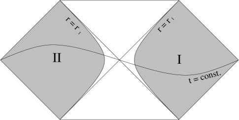
Figure 1: The Kruskal-like extension of the static, spherically symmetric black-hole spacetime. We consider only the regions satisfying $r>r_{1}$ (the shaded regions $I$ and $II$ ).

In this situation, there is a natural choice for division of the system of the scalar field: let ${\cal H}_{I}$ be the space of mode functions with supports in the region $I$ and ${\cal H}_{II}$ be the space of mode functions with supports in the region $II$. Thence, the space ${\cal F}$ of all states are of the form (2), where ${\cal F}_{I}$ and ${\cal F}_{II}$ are defined as symmetric Fock spaces constructed from ${\cal H}_{I}$ and ${\cal H}_{II}$, respectively:

$${\cal F}_{I} \equiv \mbox{\boldmath C}\oplus{\cal H}_{I}\oplus\left({\cal H}_{I}\bar{\otimes}{\cal H}_{I}\right)_{sym}\oplus\cdots,$$

$${\cal F}_{II} \equiv \mbox{\boldmath C}\oplus{\cal H}_{II}\oplus\left({\cal H}_{II}\bar{\otimes}{\cal H}_{II}\right)_{sym}\oplus\cdots.$$ (8)

Here $(\cdots)_{sym}$ denotes the symmetrization.

III Small backreaction condition

Let us investigate what kind of condition should be imposed for our arguments to be self-consistent. A clear condition is that the backreaction of the scalar field to the background geometry should be finite. For the brick wall model this condition is satisfied. Namely, in Ref. Mukohyama&Israel , it was shown that the total mass of the thermal atmosphere of quantum fields is actually bounded. Thus, also for our system, we would like to impose the condition that the contribution $\Delta M$ of the subsystem ${\cal F}_{I}$ to the mass of the background geometry should be bounded in the limit $\alpha\to 0$.

It is easily shown that $\Delta M$ is given by

$$\Delta M\equiv-\int_{x\in I}T^{t}_{t}4\pi r^{2}dr=H_{I},$$ (9)

where $H_{I}$ is the Hamiltonian of the subsystem ${\cal F}_{I}$ with respect to the Killing time $t$. Hence, the expectation value of $\Delta M$ with respect to a state $|\psi\rangle$ of the scalar field is decomposed into the contribution of excitations and the contribution from the zero-point energy:

$$\langle\psi|\Delta M|\psi\rangle=E_{ent}+\Delta M_{B},$$ (10)

where $E_{ent}$ is entanglement energy defined by

$$E_{ent}\equiv\langle\psi|:H_{I}:|\psi\rangle,$$ (11)

and $\Delta M_{B}$ is the zero-point energy of the Boulware state. Here, the colons denote the usual normal ordering. [This definition of entanglement energy corresponds to $E_{ent}^{(I^{\prime})}$ in Ref. MSK1998 and $\langle:H_{2}:\rangle$ in Ref. D-thesis .]

Since the Boulware energy $\Delta M_{B}$ diverges as $\Delta M_{B}\sim-AT_{H}\alpha^{-2}$ in the limit $\alpha\to 0$ Mukohyama&Israel , we should impose the condition

$$E_{ent}\simeq|\Delta M_{B}|,$$ (12)

where $A=4\pi r_{0}^{2}$ is the area of the horizon, $T_{H}=\kappa_{0}/2\pi$ is the Hawking temperature. We would like to call this condition the small backreaction condition (SBC). Note that the right hand side of SBC (12) is independent of the state $|\psi\rangle$.

IV Maximal entanglement entropy

Now, we shall show that the Hartle-Hawking state is a maximum of the entanglement entropy in the space of quantum states satisfying SBC. For this purpose, we prove a more general statement for a quantum system with a state-space of the form (2): a state of the form

$$|\psi\rangle={\cal N}\sum_{n}e^{-E_{n}/2T}|n\rangle_{I}\otimes|n\rangle_{II}$$ (13)

is a maximum of the entanglement entropy in the space of states with fixed expectation value of the operator $E_{I}$ defined by

$$E_{I}=\left(\sum_{n}E_{n}|n\rangle_{I}\cdot{}_{I}\langle n|\right)\otimes\left(\sum_{m}|m\rangle_{II}\cdot{}_{II}\langle m|\right),$$ (14)

provided that the real constant $T$ is determined so that the expectation value of $E_{I}$ is actually the fixed value. Here, $\{|n\rangle_{I}\}$ and $\{|n\rangle_{II}\}$ ($n=1,2,\cdots$) are bases of the subspaces ${\cal F}_{I}$ and ${\cal F}_{II}$, respectively, and $E_{n}$ are assumed to be real and non-negative. Note that this statement is almost the same as the following statement in statistical mechanics: a canonical state is a maximum of statistical entropy in the space of states with fixed energy, provided that the temperature of the canonical state is determined so that the energy is actually the fixed value.

Note that the expectation value of $E_{I}$ is equal to the entanglement energy (11), providing that $|n\rangle_{I}$ and $E_{n}$ are an eigenstate and an eigenvalue of the normal-ordered Hamiltonian $:H_{I}:$ of the subsystem ${\cal F}_{I}$. Hence, for the system of the scalar field, the above general statement insists that the state (13) is a maximum of the entanglement entropy in the space of states satisfying SBC, which corresponds to fixing the entanglement entropy. Off course, in this case, the constant $T$ should be determined so that SBC (12) is satisfied.

Returning to the subject, let us prove the general statement. (The following proof is the almost same as that given in the Appendix of Ref. Mukohyama1998 for a slightly different statement. However, for completeness, we shall give the proof. )

First, we decompose an element $|\psi\rangle$ of ${\cal F}$ as

$$|\psi\rangle=\sum_{n,m}C_{nm}|n\rangle_{I}\otimes|m\rangle_{II},$$ (15)

where the coefficients $C_{nm}$ ($n,m=1,2,\cdots$) are complex numbers satisfying $\sum_{n,m}|C_{nm}|^{2}=1$ and can be considered as matrix elements of a matrix $C$. Since $C^{\dagger}C$ is a non-negative Hermitian matrix, it can be diagonalized as

$$C^{\dagger}C=V^{\dagger}PV,$$ (16)

where $P$ is a diagonal matrix with diagonal elements $p_{n}$ ($\geq 0$) and $V$ is a unitary matrix. For this decomposition and diagonalization, the entanglement entropy and the expectation value of the operator $E_{I}$ are written as follows.

$$S_{ent} = -\sum_{n}p_{n}\ln p_{n},$$ (17)

$$E_{ent} = \sum_{n,m}E_{n}p_{m}|V_{nm}|^{2},$$ (18)

where $V_{nm}$ is matrix elements of $V$. The constraints $\sum_{n,m}|C_{nm}|^{2}=1$ and $V^{\dagger}V={\bf 1}$ are equivalent to

$$\sum_{n}p_{n} = 1,$$

$$\sum_{l}V^{*}_{ln}V_{lm} = \delta_{nm}.$$ (19)

Next, we shall show that these expressions are equivalent to those appearing in statistical mechanics in ${\cal F}_{I}$. Let us consider a density operator $\bar{\rho}$ on ${\cal{F}}_{I}$:

$$\bar{\rho}=\sum_{n,m}\tilde{P}_{nm}|n\rangle_{I}\cdot{}_{I}\langle m|,$$ (20)

where $(\tilde{P}_{nm})$ is a non-negative Hermitian matrix with unit trace. By diagonalizing the matrix $\tilde{P}$ as

$$\tilde{P}=\bar{V}^{\dagger}\bar{P}\bar{V},$$ (21)

we obtain the following expressions for entropy $S$ and an expectation value $E$ of the operator $\bar{E}_{I}\equiv\sum_{n}E_{n}|n\rangle_{I}\cdot{}_{I}\langle n|$.

$$S = -\sum_{n}\bar{p}_{n}\ln\bar{p}_{n},$$

$$E = \sum_{n}\sum_{n,m}E_{n}\bar{p}_{m}|V_{nm}|^{2},$$ (22)

where $\bar{p}_{n}$ is the diagonal elements of $\bar{P}$. The constraints $\bf{Tr}\bar{\rho}=1$ and $\bar{V}^{\dagger}\bar{V}={\bf 1}$ are restated as

$$\sum_{n}\bar{p}_{n} = 1,$$

$$\sum_{l}\bar{V}^{*}_{ln}\bar{V}_{lm} = \delta_{nm}.$$ (23)

From these and those expressions, the following correspondence is easily seen:

$$S_{ent} \leftrightarrow S,$$

$$E_{ent} \leftrightarrow E,$$

$$C^{\dagger}C \leftrightarrow \tilde{P}.$$ (24)

Hence, a maximum of $S$ in the space of statistical states with a fixed value of $E$ gives a set of maxima of $S_{ent}$ in the space of quantum states with a fixed value of $E_{ent}$. (All of them are related by unitary transformations in the subspace ${\cal F}_{II}$.) Thus, since the thermal state $\tilde{P}_{nm}=e^{-E_{n}/T}\delta_{nm}$ is a maximum of $S$ in the space of statistical states with a fixed value of $E$, $C_{nm}=e^{-E_{n}/2T}\delta_{nm}$ is a maximum of $S_{ent}$ in the space of quantum states with a fixed value of $E_{ent}$. Here the temperature (or the constant) $T$ should be determined so that $E$ (or $E_{ent}$) has the fixed value. This completes the proof of the general statement.

Therefore, for the system of the scalar field, a state of the form (13) is a maximum of the entanglement entropy in the space of quantum states satisfying SBC, provided that the constant $T$ is determined so that SBC is satisfied. The value of $T$ is easily determined as $T=T_{H}$ by using the well-known fact that the negative divergence in the Boulware energy density can be canceled by thermal excitations if and only if temperature with respect to the time $t$ is equal to the Hawking temperature.

Finally, we obtain the statement that the Hartle-Hawking state Hartle&Hawking is a maximum of entanglement entropy in the space of quantum states satisfying SBC since the Hartle-Hawking state is actually of the form (13) with $T=T_{H}$ Israel1976 . [Strictly speaking, in order to obtain the Hartle-Hawking state, we have to take the limit $\alpha\to 0$ (and $L\to\infty$). However, the following arguments still hold for a finite value of $\alpha$ (and $L$).] The corresponding reduced density matrix is the thermal state with temperature equal to the Hawking temperature. Therefore, the maximal entanglement entropy is equal to the thermal entropy with the Hawking temperature, which is sought in the brick wall model.

V Conclusion

In summary the brick wall model seeks the maximal value of entanglement entropy. In other words, the entanglement approach reduces to the brick wall model when we seek the maximal entanglement entropy .

Our arguments suggests strong connection among three kinds of thermodynamics: black hole thermodynamics, statistical mechanics, and entanglement thermodynamics Mukohyama1998 ; MSK1998 ; D-thesis ; MSK1997 . It will be interesting to investigate close relations among them in detail.

- (1) J. D. Bekenstein, Phys. Rev. D7, 949 (19973).
- (2) S. W. Hawking, Commun. Math. Phys. 43, 199 (1975).
- (3) L. Bombelli, R. K. Koul, J. Lee and R. D. Sorkin, Phys. Rev. D34, 373 (1986).
- (4) M. Srednicki, Phys. Rev. Lett. 71, 666 (1993).
- (5) G. ’tHooft, Nucl. Phys. B256, 727 (1985).
- (6) S. Mukohyama and W. Israel, Phys. Rev. D58, 104005 (1998).
- (7) S. Mukohyama, M. Seriu and H. Kodama, Phys. Rev. D58, 064001 (1998).
- (8) S. Mukohyama, “The origin of black hole entropy”, Doctoral thesis, gr-qc/9812079.
- (9) S. Mukohyama, Phys. Rev. D58, 104023 (1998).
- (10) J. B. Hartle and S. W. Hawking, Phys. Rev. D13, 2188 (1976).
- (11) W. Israel, Phys. Lett. 57A, 107 (1976).
- (12) S. Mukohyama, M. Seriu and H. Kodama, Phys. Rev. D55, 7666 (1997).
- (13) S. Mukohyama, “Hartle-Hawking state is a maximum of entanglement entropy“, gr-qc/9904005.