Global solutions in gravity.
Lorentzian signature.

Abstract

The constructive method of conformal blocks is developed for the construction of global solutions for two-dimensional metrics having one Killing vector. The method is proved to yeild a smooth universal covering space with a smooth pseudo-Riemannian metric. The Schwarzschild, Reisner–Nordstrom solutions, extremal black hole, dilaton black hole, and constant curvature surfaces are considered as examples.

1 Introduction

A space-time in gravity models is a differentiable manifold which has to satisfy at least two requirements. Firstly, the Lorentz signature metric satisfying some system of equations of motion is to be given on it. Secondly, the manifold has to be maximally extended along extremals. The last requirement means that any extremal can be either continued to infinite value of the canonical parameter in both directions or at a finite value of the canonical parameter it ends up at a singular point where one of the geometric invariants, for example, the scalar curvature becomes infinite. Space-time with a given metric satisfying both requirements is called a global solution in gravity. This definition is invariant and do not depend on the coordinate system because the canonical parameter is invariant and defined up to a linear transformation. The Kruskal–Szekeres extention [1, 2] of the Schwarzschild solution [3] is a well known example of nontrivial global solution in general relativity.

The necessity to construct global solutions, that is, manifolds themselves and metrics given on them, is related to the invariance of gravity models under general coordinates transformations. As a rule some coordinates are fixed when solving the equations of motion, and this reduces the number of unknown functions. On the other hand fixing of the coordinate system means that excluding trivial examples the obtained solution is a local one and represents only a part of some larger space-time. Note also that only the global structure of a manifold allows one to give the physical interpretation of a solution to the equations of motion for the metric because it is invariant.

The problem setting by itself differs from standard problems in mathematical physics where a manifold is assumed to be given in advance, and the task is to solve one or the other boundary value problem. In contrast to this the boundary conditions are replaced by the requirement of completeness, and the manifold by itself is constructed along with the equations solving. It is interesting to analyse the relation between the theory of global solutions and general theory of dynamical systems, the basics of which were founded by N. N. Bogolubov [4].

Construction of global solutions in gravity is a difficult problem because besides a solution of the equations of motion which is a difficult task by itself includes solution of the equations for extremals analisys of their completeness, and extention of the manifold in the case of its incompleteness. In general relativity only a small number of global solutions is known in account of the complicated equations of motion (see review [5]). In two-dimensional gravity models attracting much interest last years the situation is simpler, and all global solutions were succeeded to be found [6] in two-dimensional gravity with torsion [7], and in a large class of dilaton gravity models too [8, 9, 10]. Constractive method of conformal blocks was proposed [6] for two-dimensional gravity with torsion in the conformal gauge, the ${\cal C}^{2}$ continuity being proved on horizons along which local solutions were sewed together. The proof was based only on the analisys of asymptotics near horizons, and therefore it is applicable to other models. The use of Eddington–Finkelstein coordinates in the analisys of global solutions for a wide class of two-dimensional models including dilaton gravity [8] allowed to prove the smoothness of global solution. Analisys of the equations of motion in general relativity showed that solutions having the form of a warped product of two surfaces can also be explicitly constructed and classified [11]. In fact, the majority of known global solutions in general relativity belong to this class.) Pricisely this allowed one to give the physical interpretation to many solutions known before only locally. That is, vacuum solutions to the Einstein equations with cosmological constant from the considered class describe black holes, wohmholes, cosmic strings, domain walls, and many other solutions of physical interest.

The method of conformal blocks is applicable for two-dimensional metrics having one Killing vector. In the present paper for an arbitrary metric of this type the constructive rules for building global solutions are formulated, smoothness and uniqueness of the global solution are proved up to diffeomorphisms and the action of descreet transformation group. In section 2 the metric is considered, and conditions following from the singularity of the scalar curvature are obtained. In section 3 the notion of the conformal blocks is introduces from which global solutions are built. In the next section 4 equations for extremals are solved, their form, asymptotics, and completeness are analysed. In section 5 the method of conformal blocks for building global solutions is proposed, and the main theorem is formulated on the smoothness of the obtained universal covering space. In section 6 the Schwarzschild, Reisner–Nordström solutions, extremal and dilaton black holes, and the constant curvature surfaces are considered as examples of the conformal blocks method. In sections 7 and 8 the proof of the main theorem is completed by the transition to coordinate systems covering horizons and saddle points.

2 Local form of the metric

Consider a plane ${\mathbb{R}}^{2}$ with Cartesian coordinates $\zeta^{\alpha}$$=\left\{\tau,\sigma\right\}$, $\alpha=0,1$. Let conformally flat metric of Lorentz signature be given in some domain in the plane

$$ds^{2}=|N(q)|(d\tau^{2}-d\sigma^{2}).$$ (1)

We consider conformal factor $N(q)\in{\cal C}^{l}$, $l\geq 2$ to be $l$ times continuously differentiable function of one argument $q\in{\mathbb{R}}$ except for a finite number of singularities. Later the smoothness class of the global metric arising after continuation of (1) will be shown to coinside with the smoothness of the conformal factor $N(q)$ between singularities. Let the argument $q$ to depend on one coordinate only, and this dependence to be given by the ordinary differenrtial equation

$$\left|\frac{dq}{d\zeta}\right|=\pm N(q),$$ (2)

with the following sign rule

$$\begin{array}[]{ccl}N>0:&~{}~{}\zeta=\sigma,&~{}~{}\text{sign $+$, (static solution)},\\ N<0:&~{}~{}\zeta=\tau,&~{}~{}\text{sign $-$, (homogeneous solution)}.\end{array}$$ (3)

The choice of the quadratic form (1), (2) will be shown in section 6 to include a wide class of metrics interesting from mathematical and physical point of view. We admit that conformal factor may have zeroes and singularities in a finite number of points $q_{i}$, $i=1,\dots,k$. The infinite points $q_{1}=-\infty$ and $q_{k}=\infty$ are also included in this sequence. We consider power behaviour of the conformal factor near $q_{i}$

$$|q_{i}|<\infty: N(q)\sim(q-q_{i})^{m},$$ (4)

$$|q_{i}|=\infty: N(q)\sim q^{m}.$$ (5)

The exponent $m$ may be an arbitrary real number, that is, the conformal factor may have, for example, branch points. At finite points $|q_{i}|<\infty$ for positive $m>0$ the conformal factor equals zero. These points will be shown to correspond to horizons of a space-time. Negative values $m<0$ correspond to singularities. At infinite points positive and negative values of $m$ correspond conversly to singularities and zeroes of the conformal factor. The following analisys may be generalized to more complicated functions $N(q)$ having, for example, logarithmic branch points. For simplicity we restrict ouselves to a power behavior (4). On the intervals between zeroes and singularities where the function $N$ is either positive or negative the solution is static with the Killing vector $K=\partial_{\tau}$ or homogeneous with the Killing vector $K=\partial_{\sigma}$, correspondingly. The length of the Killing vector equals $N(q)$ in both cases.

Note that under the conformal transformations the form of the metric (1), (2) changes because the argument $q$ becomes a function of both coordinates on the plane. Under the scale transformations $\zeta^{\prime}=k\zeta$, $k={\sf const}\neq 0$, which form a subgroup of the conformal group the metric preserve its form if $q^{\prime}=k^{-1}q$ and $N^{\prime}=k^{-2}N$.

In fact formulae (1) and (2) define four different metrics, due to the modulus sign on the derivative in (2) there are two domains with static metric and two domains with homogeneous metric differing by the sign of the derivative $dq/d\zeta$. Denote these domains by the Roman digits

$$\begin{array}[]{rcl}\text{I}:{}{}&N>0,{}{}&dq/d\sigma>0,\\ \text{II}:{}{}&N<0,{}{}&dq/d\tau<0,\\ \text{III}:{}{}&N>0,{}{}&dq/d\sigma<0,\\ \text{IV}:{}{}&N<0,{}{}&dq/d\tau>0.\end{array}$$ (6)

The order of the domains will be clear from the following considerations. Note that the static solution in the domain III is obtained by the space reflection $\sigma\rightarrow-\sigma$ from that in the domain I, and homogeneous solution in the domain IV is related by time reflection $\tau\rightarrow-\tau$ to the solution in the domain II. As far as changing the sign of the conformal factor may be compensated by exchanging space and time coordinates $\tau\leftrightarrow\sigma$, then homogeneous solutions in domains II and IV may be obtained from static solutions for the conformal factor $-N$ in domains III and I with the following rotation of the $\tau,\sigma$ plain by the angle $\pi/2$ clockwise.

The Schwarzschild metric is an example of the type (1). Indeed, in static domains I and III make the coordinate transformation $\tau,\sigma$ $\rightarrow$ $\tau,q$. Then the metric takes the form

$$ds^{2}=N(q)d\tau^{2}-\frac{dq^{2}}{N(q)},~{}~{}~{}~{}~{}~{}N>0.$$ (7)

Neglecting the angular part in the Schwarzschild metric one gets the metric (7) for

$$N(q)=1-\frac{2M}{q},$$ (8)

where $M={\sf const}$ is the mass of the black hole, and the coordinate $q$ may be interpreted as the radius. In the considered case the function $N(q)$ has simple pole at $q=0$ and simple zero (horizon) at the point $q=2M$. In the homogeneous domains II and IV one can make anologous transformation of the coordinates $\tau,\sigma$ $\rightarrow$ $q,\sigma$. Then the metric becomes

$$ds^{2}=-\frac{dq^{2}}{N(q)}+N(q)d\sigma^{2},~{}~{}~{}~{}~{}~{}N<0.$$ (9)

In these domains the coordinate $q$ is timelike and can not be interpreted as the radius. Coordinates $\tau,q$ and $q,\sigma$ are called Schwarzschild coordinates. Metric in these coordinates has a simple form, all functions being given explicitly. The disadvantage of the coordinates is that they do not distinguish domains I, III and II, IV. This is essential, because all domains must be used for the construction of a global solution.

Christoffel’s symbols for the metric (1) are different in different domains. Explicit expressions for nonzero components only are

$$\text{I}: \Gamma_{\tau\tau}{}^{\sigma}=\Gamma_{\tau\sigma}{}^{\tau}=\Gamma_{\sigma\tau}{}^{\tau}=\Gamma_{\sigma\sigma}{}^{\sigma}=\frac{1}{2}N^{\prime},$$ (10)

$$\text{II}: \Gamma_{\tau\tau}{}^{\tau}=\Gamma_{\tau\sigma}{}^{\sigma}=\Gamma_{\sigma\tau}{}^{\sigma}=\Gamma_{\sigma\sigma}{}^{\tau}=\frac{1}{2}N^{\prime},$$ (11)

$$\text{III}: \Gamma_{\tau\tau}{}^{\sigma}=\Gamma_{\tau\sigma}{}^{\tau}=\Gamma_{\sigma\tau}{}^{\tau}=\Gamma_{\sigma\sigma}{}^{\sigma}=-\frac{1}{2}N^{\prime},$$ (12)

$$\text{IV}: \Gamma_{\tau\tau}{}^{\tau}=\Gamma_{\tau\sigma}{}^{\sigma}=\Gamma_{\sigma\tau}{}^{\sigma}=\Gamma_{\sigma\sigma}{}^{\tau}=-\frac{1}{2}N^{\prime},$$ (13)

where prime denotes the derivative with respect to $q$. In static and homogeneous domains nonzero Christoffel’s symbols have odd number of space and time indices, respectively. In static and homogeneous domains Christoffel’s symbols differ by the sign. This is the consequence of the fact that domains of one type are related by the transformation $\zeta\rightarrow-\zeta$, and Christoffel’s symbols are linear in derivatives. The curvature tensor has only four nonzero components in every domain

$$\text{I,~{}III}: R_{\tau\sigma\tau}{}^{\sigma}=-R_{\sigma\tau\tau}{}^{\sigma}=R_{\tau\sigma\sigma}{}^{\tau}=-R_{\sigma\tau\sigma}{}^{\tau}=-\frac{1}{2}N^{\prime\prime}N,$$ (14)

$$\text{II,~{}IV}: R_{\tau\sigma\tau}{}^{\sigma}=-R_{\sigma\tau\tau}{}^{\sigma}=R_{\tau\sigma\sigma}{}^{\tau}=-R_{\sigma\tau\sigma}{}^{\tau}=~{}~{}\frac{1}{2}N^{\prime\prime}N.$$ (15)

The Ricci tensor has two nonvanishing components

$$\text{I,~{}III}: R_{\tau\tau}=-R_{\sigma\sigma}=-\frac{1}{2}N^{\prime\prime}N,$$ (16)

$$\text{II,~{}IV}: R_{\tau\tau}=-R_{\sigma\sigma}=\frac{1}{2}N^{\prime\prime}N.$$ (17)

And the scalar curvature is the same in all four domains

$$\text{I,~{}II,~{}III,~{}IV}:~{}~{}R=-N^{\prime\prime}.$$ (18)

This is an algebraic equation relating $q$ and $R$ for a given conformal factor $N$. As the consequence one gets that the function $q=q(\tau,\sigma)$, as long as the scalar curvature may be considered as a scalar function. That is equation (18) can be considered as an invariant definition of the function $q(\zeta)$ in an arbitrary coordinate system. In the domain where equation (18) can be solved with respect to $q$, the scalar curvature $R$ may be chosen as one of the coordinates.

Maximal extension means that if a surface has a boundary lying at a finite distance, that is corresponding to a finite value of the canonical parameter, then the boundary may be only singular where the scalar curvature becomes infinite. In the opposite case a manifold could be continued. For constant curvature surfaces to be discussed in detail in section 6.7 the conformal factor is a quadratic polynomial

$$N(q)=-(aq^{2}+bq+c),~{}~{}~{}~{}~{}~{}a,b,c={\sf const}.$$ (19)

Here $R=2a$.

As the consequence of equation (18) the scalar curvature is singular near $q_{i}$ for the following exponents in asymptotic behaviour (4):

$$|q_{i}|<\infty: m<0,~{}~{}0<m<1,~{}~{}1<m<2,$$ (20)

$$|q_{i}|=\infty: m>2.$$ (21)

At infinite points $q\rightarrow\pm\infty$ the scalar curvature tends to a nonzero constant for $m=2$ and to zero for $m<2$.

3 Conformal blocks

The notion of the conformal block corresponding to every interval $(q_{i},q_{i+1})$ will be used in building of global solutions. Inside the interval the conformal factor $N$ is either strictly positive or strictly negative. Let us find the domain of definition for the metric (1) on the $\tau,\sigma$ plain. For definiteness we consider static solution I on the interval $(q_{i},q_{i+1})$. Then the time coordinate takes values on the whole real axis $\tau\in{\mathbb{R}}$. Equation (2) for the space coordinate $\sigma$ becomes

$$\frac{dq}{d\sigma}=N(q).$$ (22)

Integration constant for this equation corresponds to a shift of the spacelike coordinate $\sigma\rightarrow\sigma+{\sf const}$, that is to the choice of the origin of $\sigma$. From equation (22) one gets that the domain of $\sigma$ depends on the convergence of the integral

$$\sigma\sim\int^{q_{i},q_{i+1}}\frac{dq}{N(q)}$$ (23)

at the boundary points. The integral (23) converge or diverge depending on the exponent $m$:

$$\begin{array}[]{rl}|q_{i}|<\infty:{}{}{}{}&\left\{\begin{array}[]{rll}m<1{}{}&\text{-- converge,}&\text{~{}~{}line,}\\ m\geq 1{}{}&\text{-- diverge,}&\text{~{}~{}angle,}\end{array}\right.\\ |q_{i}|=\infty:{}{}{}{}&\left\{\begin{array}[]{rll}m\leq 1{}{}&\text{-- diverge,}&\text{~{}~{}angle,}\\ m>1{}{}&\text{-- converge,}&\text{~{}~{}line.}\end{array}\right.\end{array}$$ (24)

At the right of this table the form of the boundary of the corresponding conformal blocks introduced below is given. If at both ends of the interval $(q_{i},q_{i+1})$ the integral diverge, then $\sigma\in(-\infty,\infty)$, and the metric is defined on the whole $\tau,\sigma$ plain. If at one of the ends $q_{i+1}$ or $q_{i}$ the integral converge, then the metric is defined on the half plain $\sigma\in(-\infty,\sigma_{i+1})$ or $\sigma\in(\sigma_{i},\infty)$, correspondingly. The choice of boundary points $\sigma_{i+1}$ and $\sigma_{i}$ is arbitrary, and without loss of generality one may set $\sigma_{i,i+1}=0$. If the integral converge on both sides of the interval, then the solution is defined on the strip $\sigma\in(\sigma_{i},\sigma_{i+1})$, and one point can be only set to zero.

For visual image of a maximally extended solution the notion of conformal block is introduced. To this end we map the $\tau,\sigma$ plain on the square along the light like directions

$$\xi=\tau+\sigma,~{}~{}~{}~{}~{}~{}\eta=\tau-\sigma.$$ (25)

For the purpose we make a conformal transformation

$$u=u(\xi),~{}~{}~{}~{}v=v(\eta),~{}~{}~{}~{}~{}~{}u,v\in{\cal C}^{l+1},$$ (26)

where the functions $u$ and $v$ are bounded, and their first derivatives are positive. Without loss of generality we consider $u,v\in[-1,1]$. The assumption about the smoothness of the transition functions preserves the smoothness of the metric after the coordinate transformation. Then the static solution defined on the whole $\tau,\sigma$ plain corresponds to a square conformal block, shown in Fig. 1,a.

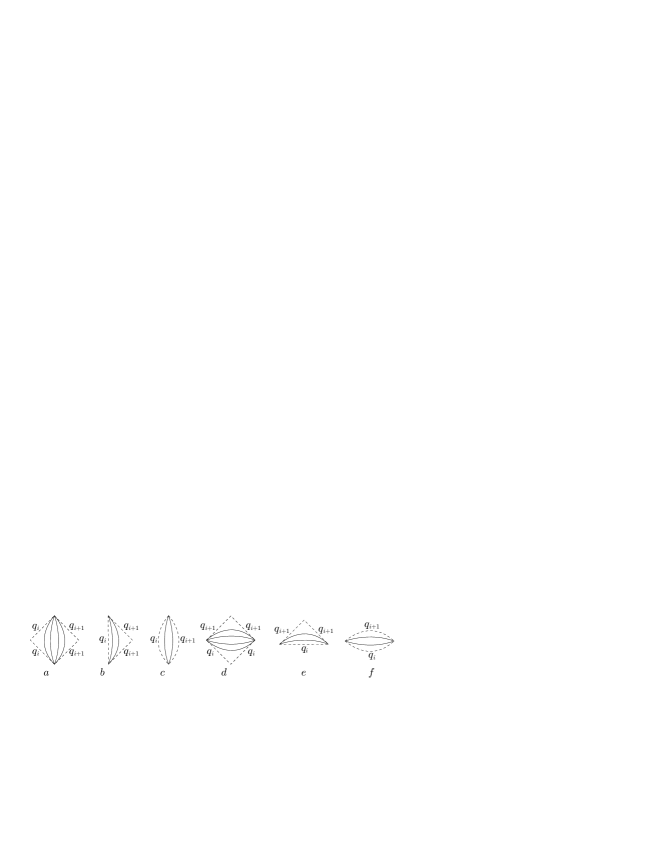
Figure 1: Conformal blocks for static (a,b,c) and homogeneous (d,e,f) solutions. Thin solid lines denote Killing trajectories. The variable $q\in(q_{i},q_{i+1})$ is constant along Killing trajectories and varies from the left boundary to the right one being constant along the boundaries. For homogeneous solutions the variable $q$ varies analogously but from bottom to top. Every conformal block has its symmetrical patner obtained by space $\sigma\leftrightarrow-\sigma$ or time $\tau\leftrightarrow-\tau$ reflection for static and homogeneous solutions, respectively.

In a general case conformal block is a finite part of the $u,v$ plain and the given metric (1) in coordinates (25), (26). If one requires the extremals to approach the boundary on all possible angles, then this uniquely determines the asymptotic behavior of the transition functions (26) [6]. In all other respects the transition functions are arbitrary. We shall not discuss this point in detail because the smoothness of the metric on the horizons will be proved by going to Eddington–Finkelstein coordinates in section 7.

The value of $q$ and, consequently, the scalar curvature is constant along time like Killing trajectories shown inside the block by thin solid lines. The variable $q$ continuoesly changes from left to right monotonically increasing in the domain I and decreasing in the domain III. It takes the value $q_{i}$ on both left sides of the square and the value $q_{i+1}$ on both right sides. Lower and upper coners of the square are essentially singular points because the limit of $q$ in these points depends on the path along which a sequence goes to the coner. We say that static conformal block has two boundaries, left and right, on which the variable $q$ takes values $q_{i}$ and $q_{i+1}$, respectively.

If solution of equation (22) is defined on the half interval, then a static solution corresponds to a triangular conformal block, an example of which is shown in Fig. 1,b. And the vertical line correspond to the boundary point $\sigma_{i}=0$. This can be always achieved by the choice of the functions $u(\xi)$ and $v(\eta)$.

When solutions of equation (22) is defined on a finite interval the conformal block is represented in the form of a lens, depicted in Fig. 1,c. The choice of the functions $u(\xi)$ and $v(\eta)$ allows one to make left or right boundary vertical but not both boundaries simultaneously.

Let us remind the reader that there are two conformal blocks for every interval because equation (2) is invariant under the space reflection $\sigma\leftrightarrow-\sigma$ due to the modulus sign.

Analogously, one of the conformal blocks shown in Fig. 1,d,e,f or its turned over partner obtained by the time inversion $\tau\leftrightarrow-\tau$ corresponds to every homogeneous solution. On these conformal blocks the variable $q$ is constant along space like Killing trajectories and monotonically increases or decreases from the value $q_{i}$ on the lower boundary to the value $q_{i+1}$ on the upper one. Left and right coners of homogeneous conformal blocks are essentially singular points.

Conformal blocks for static and homogeneous solutions are called static and homogeneous, respectively.

Thus we have shown that a Lorenzian surface with a given conformally flat metric (1) is diffeomorphic to one of the conformal blocks. To construct maximally extended solutions one has to find and analyse extremals on these surfaces, in the case of necessity to extend the manifold and the metric, and to prove the smoothness. The use of the conformal blocks in construction of global solutions is convenient because all light like extremals are depicted as two classes of straight lines going by the angle $\pm\pi/4$ to the time axis. Therefore gluing conformal blocks along edges preserves the smoothness of light like extremals.

4 Extremals

4.1 The form of the extremals

To understand the global structure of a solution for metric (1) one has to analyse the behavior of extremals $\zeta^{\alpha}(t)=\left\{\tau(t),\sigma(t)\right\}$ satisfying in general the system of equations

$$\ddot{\zeta}^{\alpha}=-\Gamma_{\beta\gamma}{}^{\alpha}\dot{\zeta}^{\beta}\dot{\zeta}^{\gamma},$$

where the dot denotes the derivative with respect to the canonical parameter $t$.

Let us analyse the behavior of extremals in the static domain

$$\text{I}:~{}~{}ds^{2}=N(q)(d\tau^{2}-d\sigma^{2}),~{}~{}~{}~{}~{}~{}\frac{dq}{d\sigma}=N(q)>0.$$ (27)

Using the expression for Christoffell’s symbols (10) we get equations for extremals

$$\ddot{\tau} = -N^{\prime}\dot{\tau}\dot{\sigma},$$ (28)

$$\ddot{\sigma} = -\frac{1}{2}N^{\prime}(\dot{\tau}^{2}+\dot{\sigma}^{2}).$$ (29)

This system of equations has two first integrals

$$N(\dot{\tau}^{2}-\dot{\sigma}^{2}) = C_{0}={\sf const},$$ (30)

$$N\dot{\tau} = C_{1}={\sf const}.$$ (31)

The integral of motion (30) has the same meaning as the possibility to choose the length of an extremal as the canonical parameter for a positive definite metric. The value of the constant $C_{0}$ defines the type of an extremal:

$$C_{0}>0 - \text{time like extremals},$$

$$C_{0}=0 - \text{light like extremals},$$

$$C_{0}<0 - \text{space like extremals}.$$

Note that the type of an extremal does not change when going from one point to another one. The second integral (31) is the consequence of the existence of a Killing vector field, that is with the symmetry of the problem, and for an arbitrary metric it does not exist.

Theorem 1

Any extremal in the static space-time of the type I, III belongs to one of the following four classes.
1) Light like extremals

$$\tau=\pm\sigma+{\sf const},$$ (32)

with the canonical parameter defined by the equation

$$\dot{\tau}=\frac{1}{N}.$$ (33)

2) General type extremals the form of which is defined by the equation

$$\frac{d\tau}{d\sigma}=\pm\frac{1}{\sqrt{1-C_{2}N}},$$ (34)

where $C_{2}$ is an arbitrary nonzero constant, the values of $C_{2}<0$ and $C_{2}>0$ defining space and time like extremals, respectively. The canonical parameter is defined by one of the two equations

$$\dot{\tau} = \frac{1}{N},$$ (35)

$$\dot{\sigma} = \pm\frac{\sqrt{1-C_{2}N}}{N}.$$ (36)

The plus or minus signs in equations (34) and (36) are to be chosen simultaneously.
3) Straight space like extremals parallel to $\sigma$ axis and going through every point $\tau={\sf const}$. The canonical parameter is defined by the equation

$$\dot{\sigma}=\frac{1}{\sqrt{N}}.$$ (37)

4) Straight degenerate time like extremals parallel to $\tau$ axis and going through the critical points $\sigma_{0}={\sf const}$ where

$$N^{\prime}(\sigma_{0})=0.$$ (38)

Their canonical parameter coinsides with the time like coordinate

$$t=\tau.$$ (39)

Proof of the theorem reduces to the integration of the system of equations (28), (29). In obtaining the integral of motion (31) one has to devide on $\dot{\tau}$ and $\dot{\sigma}$, therefore these degenerate cases must be considered seperately. For $\tau={\sf const}$ equation (28) is trivially fullfield, and equation (29) after integration yeilds

$$-N\dot{\sigma}^{2}=C_{0}\neq 0.$$

This equations is reduced to (37) by the scaling of the canonical parameter.

The second degenerate case corresponds to $\dot{\sigma}=0$. Hence equation (29) is fullfilled only in those points $\sigma=\sigma_{0}$ where $N^{\prime}(\sigma_{0})=0$ and equation (28) reduces to the equation $\ddot{\tau}=0$. Therefore the $\tau$ coordinate can be chosen as the canonical parameter. One may note the validity of the equality

$$\frac{dN}{d\sigma}=N\frac{dN}{dq}=0,$$

and differentiation with respect to $q$ in the equation (38) can be changed to the differentiation with respect $\sigma$ because $N\neq 0$. In this way all special cases are exhausted.

The remaining cases are obtained from the analysis of the integrals (30), (31), the constant $C_{0}$ being arbitrary and $C_{1}\neq 0$, since the case $C_{1}=0$ is related to the extremals of the third class. Equation (30) with (31) yeilds

$$\dot{\sigma}=\pm\frac{C_{1}}{N}\sqrt{1-C_{2}N},$$ (40)

where

$$C_{2}=\frac{C_{0}}{C_{1}^{2}}.$$ (41)

The equation for the form of a general type extremals (34) is the consequence of (31) and (40), the value of the constant $C_{2}$ defining the type of an extremal. The equation for the canonical parameter is obtained from (31) and (40) after rescaling. In a particular case $C_{2}=0$ one gets the light like extremals (32). $\Box$

As the consequence of equation (34) one gets that the constant $C_{2}$ parametrizes the angle at which the extremal goes through a given point. One may check that through every point in any direction goes one and only one extremal.

Tipical behaviour of the conformal factor with one and three local extrema between two zeroes and with two local extrema between a zero and a singularity for static conformal blocks is shown in Fig. 2 in the first row.

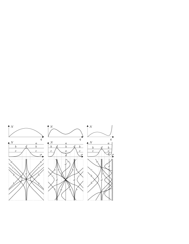
Figure 2: The first raw: tipical behaviour of the conformal factor $N(q)$ between two zeroes and a zero and a singularity for a static solution. The second raw: the dependence of the conformal factor $N(\sigma)$ on the space like coordinate. The third raw: tipical time and space like extremals. The letters mark time like extremals having qualitatively different behaviour for different values of the constant $C_{2}$. Through any local extrema goes one degenerate extremal (d). There are oscillating extremals (o) in the second and third cases.

The dependence of the conformal factors on the space like coordinate is shown in the second raw. The qualitative behaviour of time and space like extremals. Not to overload the figure light like extremals going through every point of the space-time are omitted. All extremals can be shifted along the time like coordinate $\tau$.

Time like general type extremals have qualitatively different behaviour for different values of the constant $C_{2}$. They are marked by the letters a,b,c and o. If both boundary points $q_{i}$ and $q_{i+1}$ of the interval are zeroes, then, as the consequence of continuity, the conformal factor $N$ has at least one maximum through which goes the degenerate extremal (d). For sufficiently large values of $C_{2}$ the extremals cross local maxima (a). If the function $N$ has a local minimum through which goes the degenerate extremal as well, then there are oscillating extremals among general type extremals which oscillate around the local minimum (o). This is the consequence of equation (34) because for positive values of $C_{2}$ the range of the coordinate $\sigma$ is given by the inequality

$$N<\frac{1}{C_{2}}.$$

Critical points $\sigma_{*}$ in which $N(\sigma_{*})=1/C_{2}$ are the turning points for a finite value $\tau=\tau_{*}$ if and only if the integral

$$\int^{\tau_{*}}d\tau=\pm\int^{\sigma_{*}}\frac{d\sigma}{\sqrt{1-C_{2}N}}$$ (42)

converges. This integral converges if the point $\sigma_{*}$ does not coinside with the local maximum. That is the turn happens for a finite value of $\tau_{*}$ and the canonical parameter as the consequence of equation (36). Corresponding nonoscillating extremals are marked by the letter (c). If the critical point coinsides with the local maximum, then the integral (42) diverges. It means that the critical point is reached at an infinite value of $\tau_{*}$ and the canonical parameter. That is the corresponding extremal (b) is complete in this direction.

The above theorem describes all extremals for static solutions. The behaviour of extremals for homogeneous solutions is similar. They are obtained by the replacement $N\rightarrow-N$, the exchange of time and space like coordinates $\tau\leftrightarrow\sigma$ and by the rotation of the whole plain by the angle of $\pi/2$.

4.2 Asymptotics of the extremals

To solve the problem whether a solution defined on the $\tau,\sigma$ plain is complete or it must be continued one has to analyze asymptotics and completeness of extremals near the boundary of a conformal block. All time like extremals for which

$$\lim_{\tau\to\pm\infty}\left|\frac{d\tau}{d\sigma}\right|>1$$

go to upper and lower corners of a conformal block if they exist. Extremals for which

$$\lim_{\sigma\to\pm\infty}\left|\frac{d\tau}{d\sigma}\right|<1$$

go to left and right corners of a conformal blaocks. The extremals with a light like asymptotics

$$\lim_{\tau,\sigma\to\pm\infty}\left|\frac{d\tau}{d\sigma}\right|=1$$

go to an edge of a square conformal block.

Let us consider asymptotics of extremals near the boundary of static conformal blocks. Any light like extremal starts and ends at the opposite edges of a square conformal block. On triangular or lens type conformal blocks a light like extremal starts or ends on a time like boundaries.

For static solutions I, III straight extremals parallel to the space like $\sigma$ axis start in the left and end in the right corner of a square conformal block. On a triangular or lens type conformal block these extremals start or (and) end on a time like boundary. Degenerate extremals and general type oscillating ones start in the lower and end in the upper corner of a conformal block.

Let us consider nonoscillating general type extremals. If a boundary of a conformal block is a horizon, $N(q_{i})=0$, $|q_{i}|<\infty$, then tangent vectors to extremals (34) have light like asimptotic behaviour

$$\lim_{q\to q_{i}}\left|\frac{d\tau}{d\sigma}\right|=1.$$

And these general type extremals go to edges of a square and not to the corners. Indeed, for extremals going to the right upper edge of a square equations (35), (36) imply

$$\frac{d\eta}{d\xi}=\frac{1-\sqrt{1-C_{2}N}}{1+\sqrt{1+C_{2}N}}.$$

As the consequense the integral

$$\int d\eta\sim\int d\xi N\sim\int^{q_{i}}dq=q_{i}$$

converges, and this corresponds to a point on the edge of a square. If time like boundary is reached at finite values of $\sigma_{i}$, then a tangent vector to a space like extremal has the asimptotics

$$\frac{d\tau}{d\sigma}\sim\frac{1}{\sqrt{N}}\to 0.$$

That is they reach the boundary $|\sigma_{i}|<\infty$ at the right angle. Time like extremals can not reach a time like boundary because the right hand side in (34) for $C_{2}>0$ becomes imaginary near the singularity. These extremals near the boundary $|\sigma_{i}|<\infty$ have a turning point for finite values of $\tau$ for the same reason as the oscillating extremals.

4.3 Completeness of extremals

Theorem 1 allows one to analyze the completeness of extremals near the boundary of a conformal block. For definiteness we consider a static solution. First of all note that degenerate extremals are always complete because their canonical parameter coinsides with the time (39). Oscillating extremals are complete as well because they make infinite number of oscillations each of them corresponding to a finite variation of a canonical parameter. If a general type extremal for $\tau\to\pm\infty$ approach the degenerate extremal then it is complete because equation (35) for the canonical parameter imply

$$\lim_{\sigma\to\sigma_{0}}t\to\int^{\infty}d\tau N(\sigma_{0})\to\infty.$$

For a stationary solution in lower and upper corners of a conformal block go only degenerate and oscillating extremals, hence they are always complete. The absence of these extremals is possible. In this case we consider these corners as complete because any time like curve has infinite length at $\tau\to\pm\infty$. This means that lower and upper corners of a stationary conformal blocks are always complete, that is they are past and future time infinities, correspondingly.

Completeness of light like extremals is defined by the equation (33) which imply

$$\lim_{\sigma\to\pm\infty}t\to\int d\sigma N=\int^{q_{i}}dq=q_{i}.$$ (43)

This means that near the boundary of a conformal block they are incomplete for finite $q_{i}$ and complete for $|q_{i}|=\infty$.

Completeness of nonoscillating general type extremals going to the boundary corresponding to $q_{i}$ follows from the equation (36)

$$\lim_{q\to q_{i}}t\to\int d\sigma\frac{N}{\sqrt{1-C_{2}N}}\sim\int^{q_{i}}\frac{dq}{\sqrt{1-C_{2}N}}.$$ (44)

Near horizons $N\rightarrow 0$ behaviour of general type extremals is the same as of light like extremals (43). The singularity $N\rightarrow\infty$ is reached by space like extremals, $C_{2}<0$, their completeness being defined by the equation

$$\lim_{q\to q_{i}}t\to\int^{q_{i}}\frac{dq}{\sqrt{N}}.$$ (45)

These extremals are incomplete at finite points $|q_{i}|<\infty$ for $m<0$. At infinite points $|q_{i}|=\infty$ space like extremals are complete for $0<m\leq 2$ and incomplete for $m>2$.

Completeness of straight extremals parallel to $\sigma$ axis is defined by equation (37) and near the boundary $q_{i}$ is given by the integral (45). This means that their completeness near singularities is the same as for general type extremals. Near zeroes they are always complete except for the case of a simple zero at a finite point where they are incomplete.

Thus completeness of all boundary elements is analysed. The summary is given in Fig. 3.

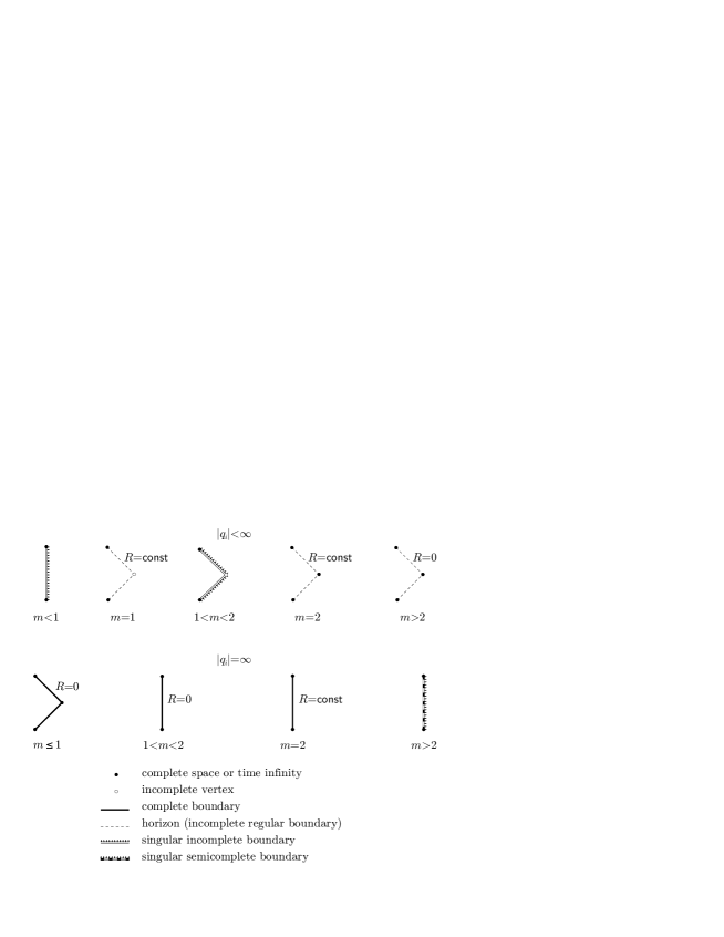
Figure 3: The form of the right boundary of the static conformal block depending on the exponent $m$. In upper and lower raws the boundaries are shown for finite and infinite values of $q_{i}$, respectively.

Here boundary elements of conformal blocks are shown depending on the exponent $m$ (4) for finite and infinite values of $q_{i}$. For definiteness we show the right boundary of static conformal blocks I. In the figure time like boundary is shown by a vertical line and light like boundary by an angle. If the scalar curvature is singular on the boundary (20), (21), then it has protuberances. Incomplete and complete boundaries are shown by dashed and thick solid lines, respectively. Exclusion is the semicomplete boundary corresponding to $|q_{i}|=\infty$ for $m>2$, Fig. 3. Light like extremals reaching this boundary are complete while space like ones are not. Lower and upper corners of all static conformal blocks (time past and future infinities) are essentially singular poits and always complete, the completeness is shown by filled circles. Completeness and incompleteness of right corners of angle boundaries are shown by filled and not filled circles, respectively. Left boundaries have the same structure, but angles should be reflected with respect to a vertical line.

Qualitative behaviour of all extremals in homogeneous space-time II, IV is defined by zeroes and singularities of the conformal factor in the same way as for a static solution. Corresponding conformal blocks should be turned by the angle $\pi/2$.

5 Construction of global solutions

In section 3 the conformal block was associated to every solution of type I-IV defined on the interval $(q_{i},q_{i+1})$. Then in section 4.3 the completeness or incompleteness of their boundaries was proved by the analysis of extremals. As a result horizons and only them turned out to correspond to boundaries incomplete with respect to extremals, the scalar curvature being finite on them. In all other cases the boundary is either complete or the curvature is singular. Therefore solutions of the form (1) must be continued only through horizons, that is the zeroes of the conformal factor. Global solutions will be depicted with the help of Carter–Penrose diagrams. Carter–Penrose diagram is a bounded image of maximally extended surface in which two classes of light like extremals are depicted as two classes of perpendicular straight lines on the Minkowskian plain. Let us formulate the rules by which maximal extension of a manifold with metric (1) for a given conformal factor $N(q)$ is realised. Smoothness and uniqueness of the manifold constructed following these rules is given by the theorem 2.

1. Every global solution for a metric (1) corresond to the interval of the variable $q\in(q_{-},q_{+})$, where $q_{\pm}$ are either infinite points or a curvature singularities defined by the condition (20). Singularities inside the interval must be absent.

2. If there are no zeroes inside the interval $(q_{-},q_{+})$ then the corresponding conformal block is the maximally extended solution.

3. If there are zeroes (horizons) inside the interval $(q_{-},q_{+})$ then enumerate them, $N(q_{j})=0$, $j=1,\dots,n$, $q_{j}\in(q_{-},q_{+})$, and associate with each of the interval $(q_{-},q_{1}),\dots,(q_{n},q_{+})$ a pare of static or homogeneous conformal blocks for $N>0$ $N<0$, respectively.

4. Sew together conformal blocks along horizons $q_{j}$, preserving the smoothness of the conformal factor, that is sew together conformal blocks corresponding only to adjacent intervals $(q_{j-1},q_{j})$ and $(q_{j},q_{j+1})$, and if the gluing is performed for static or homogeneous conformal blocks, then sew together blocks of one type.

5. The Carter–Penrose diagram obtained by gluing all adjacent conformal blocks is a connected fundamental region if inside the interval $(q_{-},q_{+})$ the conformal factor changes its sign. If $N\geq 0$ or $N\leq 0$ everywhere inside the interval $(q_{-},q_{+})$ then one gets two fundamental regions related by space or time reflection.

6. For one zero of an odd degree the boundary of the fundamental region consists of boundaries of the conformal blocks corresponding to the points $q_{-}$ and $q_{+}$, and the Carter–Penrose diagram represents the global solution.

7. If there is one zero of even degree or two or more zeroes of arbitrary degree the boundary of the fundamental region includes horizons, and it has to be either continued periodically in space and (or) time or the opposite sides should be identified.

8. If the fundamental group of the Carter–Penrose diagram is trivial then it is the universal covering space for a global solution.

9. If the fundamental group of the Carter–Penrose diagram is nontrivial, then construct the corresponding universal covering space.

The statement 1) is the consequence of impossibility to continue the solution through the points $q_{\pm}$ because these points are either complete or singular. Solutions are extended only through horizons $|q_{j}|<\infty$ with $m=1$ or $m\geq 2$. In these cases the boundary of a conformal block is an angle. If the value $q_{j}$ corresponds to an odd zero, then all four conformal blocks for the intervals $(q_{j-1},q_{j})$ and $(q_{j},q_{j+1})$ are sewed together according to the rules 3) and 4) around the vertex $q_{j}$, this point being the saddle point. If $q_{j}$ is a zero of even degree then the regions of one type are only sewed together along horizons. If inside the interval $(q_{-},q_{+})$ the function $N$ does not change the sign, then two disconnected fundamental regions appear, each of them can be periodically continued. When $N$ changes its sign the saddle point appear, and regions of different types form one fundamental region which can be either periodically continued or not depending on the value of $q$ on the boundary. This is the meaning of the rules 5) and 6). Let us formulate the main theorem justifying the above mentioned rules for construction of global solutions.

Theorem 2

The universal covering space constructed according to the rules 1)–9) is the maximally extended pseudo riemannian ${\cal C}^{l+1}$ manifold with the continuous ${\cal C}^{l}$, $l\geq 2$, metric such that every point not lying on the horizon has a neighbourhood diffeomorphic to some domain with the metric (1).

Proof. By construction the interiour of a conformal block is covered by one chart and is a ${\cal C}^{l+1}$ manifold as the consequence of (26). Therefore inside a conformal block the metric is of the same class as the conformal factor. The transition functions (26) isometrically map the $\tau,\sigma$ plain on the interior of the conformal block. Therefore one has to prove the smoothness of manifold and metric on the horizons and saddle points only. This is done in sections 7 and 8, respectively. The uniqueness of the resulting manifold follows from the well known theorem from algebraic topology stating that every manifold with nontrivial fundamental group has a unuque universal covering space up to diffeomorphisms (see, for example, [12]). $\square$

Before concluding the proof of the theorem we consider several examples to clear how to use the rules for construction of global solutions, and what kind of solutions may appear.

6 Examples

If the metric of the form (1) is obtained as the result of solution of some equations of motion, then following the rules 1)–9) from the preceeding section one can construct the global solution do not worring about going to new coordinate systems covering larger domains. The advantage of the method is that elementary analysis of the conformal factor $N(q)$ is sufficient for construction of global solutions. We start from three well known examples from general relativity.

6.1 Schwarzschild solution

The conformal factor for the Schwarzschild solution has the form (8) with $M>0$. It has a simple pole at $q=0$, $m=-1$, which corresponds to curvature singularity (20). The point $q_{1}=2M$, $m=1$, is a simple zero and corresponds to a horizon. The values $q=\pm\infty$, $m=0$, correspond to asymptotically flat space infinity. The behaviour of the conformal factor is shown in Fig. 4.

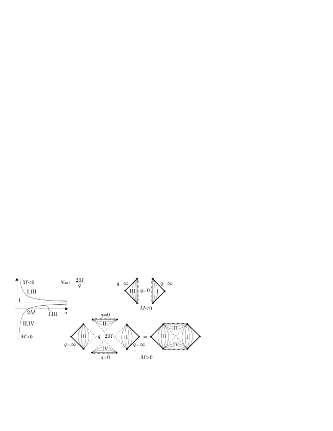
Figure 4: The behavior of the conformal factor for the Schwarzschild solution for positive and negative mass. For $M<0$ there are two global solutions depicted by triangular Carter–Penrose diagrams. For $M>0$ four conformal blocks corresponding to two intervals $(0,2M)$ $(2M,\infty)$ are sewed together in one global solution.

We see that two global solutions for positive and negative $q$ correspond to the infinite interval $q\in(-\infty,\infty)$. For positive $q\in(0,\infty)$ one has $q_{-}=0$, $q_{1}=2M$ and $q_{+}=\infty$. For each interval $q\in(0,2M)$ and $q\in(2M,\infty)$ there are two homogeneous and static conformal blocks depicted in Fig. 4. The boundary elements are defined in Fig. 3. The global solution shown in Fig. 4 is uniquely constructed by gluing together these four conformal blocks according to the rule 4). This Carter–Penrose diagram represents the Kruskal–Szekeres extention of the Schwartzschild solution. Let us remind that the Kruskal–Szekeres extention is the Schwarzschild metric written in such a coordinate system which covers all domains I–IV. Carter was the first who depicted this extension as the bounded region on the plain [5].

The constructed global solution is the unique, up to diffeomorphisms, universal covering space because its fundamental group is trivial, and part of it, namely, the domain I or III is diffeomorphic to the Schwarzschild solution.

Similar global solutions one will have for a wide class of metrics with the conformal factor having qualitatively the same form as the lower branch in Fig. 4. That is the conformal factor is defined on an infinite half-interval $(q_{-},\infty)$, has singularity at $q_{-}$, one zero, and goes to a constant at infinity. The theorem 2 quarantees the uniqueness and smoothness of the global solution, and one does not need to find global coordinates explicitly.

Note that the surface represented by the Carter–Penrose diagram has nonconstant scalar curvature

$$R=\frac{4M}{q^{3}}.$$ (46)

This is the two-dimensional scalar curvature on the Lorentz surface. The scalar curvature for a four-dimensional metric with the angular dependence is identically zero due to Einstein’s equations. Note that the two-dimensional scalar curvature (46) coinsides with the invariant eigen value of four dimensional Weyl tensor [13]. The center of the Carter–Penrose diagram is the saddle point for variable $q$ and, consequently, for the scalar curvature (46). This point is incomplete and denoted by the unfilled circle.

For negative values of $q$ horizons are absent. Therefore triangular conformal blocks shown in Fig. 4 represent maximally extended solutions. In this space-time the curvature singularity is along the time like boundary lying at a finite distance and is not surrounded by a horizon. Singularities of this type are called naked. Global solution for negative $q$ can be considered as a global solution for positive $q$ allowing one to interpret the coordinate $q$ as the radius but with negative mass $M<0$. These solutions are considered as unphysical.

6.2 Reissner–Nordström solution

The conformal factor for the Reissner–Nordström solution describing a charged black hole has the form

$$N=1-\frac{2M}{q}+\frac{Q^{2}}{q^{2}},~{}~{}~{}~{}~{}~{}0<Q<M,$$ (47)

where $M$ and $Q$ are the mass and charge of the black hole. The function $N$ for a given relation between the constants can be written in the form

$$N=\frac{(q-q_{1})(q-q_{2})}{q^{2}},$$ (48)

where

$$q_{1,2}=M\pm\sqrt{M^{2}-Q^{2}}.$$

Consequently, the conformal factor has double pole at $q=0$ and two simple zeroes (horizons) at $q_{1,2}$. Its behaviour is shown in Fig. 5.

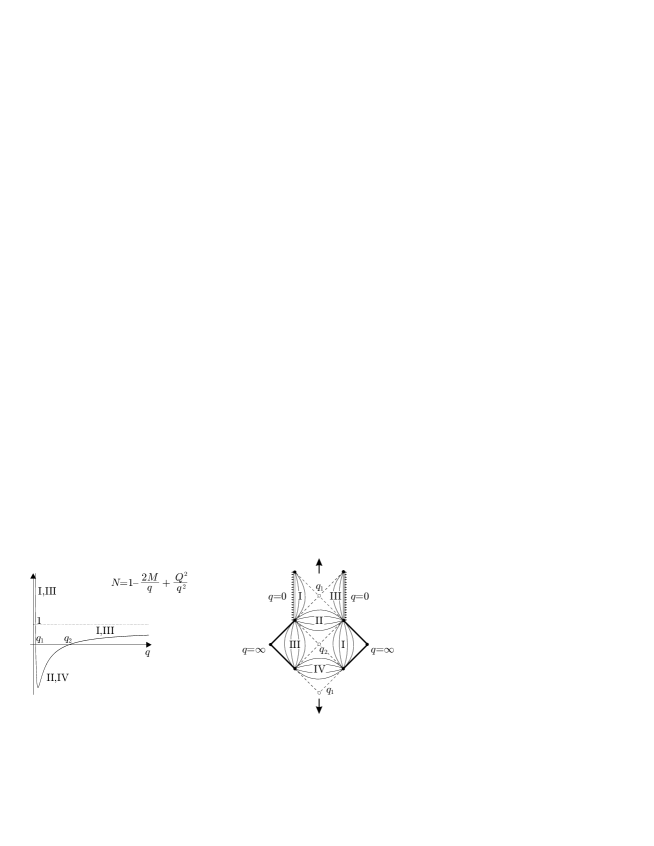
Figure 5: The conformal factor and the fundamental region for the Reissner–Nordström solution. Arrows show possible extension or identification of the solution along horizonz.

The left branch of the conformal factor corresponds to a naked singularity and will be not considered because the change of the order of the pole does not affect the structure of the global solution. Global structure of the solution for positive $q$ changes qualitatively as compared to the Schwarzschild solution due to the existence of two horizons. There are two conformal blocks for each of the intervals $(0,q_{1})$, $(q_{1},q_{2})$, and $(q_{2},\infty)$. According to the rule 6) the Carter–Penrose diagram glued from six conformal blocks and shown in Fig. 5 represents the unique fundamental region for the Reissner–Nordström solution because the conformal factor changes its sign inside the interval $(0,\infty)$. Its boundary consists not only from the singular and infinite points but includes also points corresponding to horizons. According to the rule 7) it can be periodically continued by gluing fundamental regions along horizons in the directions shown by arrows. In this case one obtains the universal covering space for the Reissner–Nordström solution. The other possibility is to identify boundary points on the lower and upper horizons after gluing together an arbitrary number of fundamental regions. Then the global solution will then be a cyllinder from topological point of view.

The scalar curvature (18) for the Reissner–Nordström solution is not constant

$$R=\frac{4M}{q^{3}}-\frac{6Q^{2}}{q^{4}}.$$ (49)

6.3 Extremal black hole

An extremal black hole appears from the Reissner–Nordström solution (47) when the mass equals to the charge $Q=M$. Corresponding conformal factor

$$N=\frac{(q-M)^{2}}{q^{2}},$$ (50)

has double pole at $q=0$ and double zero at $q=M$. Its behaviour is shown in Fig. 6.

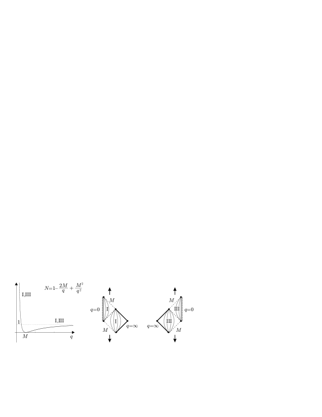
Figure 6: Conformal factor and two fundamental regions for an extremal black hole. Arrows show directions along which solutions can be continued periodically.

The left branch as in the previous cases describes a naked singularity. Positive values of $q$ are devided on two intervals $(0,M)$ and $(M,\infty)$. Two conformal blocks and their space reflection correspond to these intervals. According to the rule 6) one has two disconnected fundamental domains shown in Fig. 6 because the conformal factor does not change the sign. The second fundamental domain built from domains of type III is obtained from the domain of type I by space reflection. As in the case of Reissner–Nordström solution the boundary of the fundamental domains includes horizons and can be either glued infinitely or identified leading to the universal covering space or cyllinders, respectively.

6.4 Two-dimensional gravity with torsion

The simplest geometrical gravity model in two-dimensional space-time yeilding second order equations of motion for the zweibein and the Lorentz connection is quadratic in curvature and torsion [7]. This model is integrable [14, 15], and all solutions are devided in two classes, the constant curvature and zero torsion surfaces and the surfaces of nonconstant curvature and nontrivial torsion. For nontrivial torsion the conformal factos has the form

$$N(q)=q\left[({\sf ln}^{2}q-2{\sf ln}q+2-\Lambda)q-A\right],$$ (51)

where $\Lambda$ is the dimensionless cosmological constant and $A$ is an arbitrary integration constant (similar to the mass in the Schwarzschild solution). Depending on the values of these constants the conformal factor may have up to three roots and this yeilds eleven types of global solutions [6]. For the sake of space we shall not reproduce these solutions here. We mension that more fine classification for two-dimensional gravity with torsion is given which takes into account the completeness not only of extremals but geodesics too (they do not coinside for nontrivial torsion). It takes also into account the existence and number of degenerate extremals and geodesics.

In the present paper for simplicity we restrict ourselves to power behaviour of the conformal factor at infinite points (5). The above analysis can be easily generalized to logarithmic behaviour of the conformal factor (51) for $q\rightarrow\infty$.

6.5 The dilaton gravity

Two-dimensional dilaton gravity model is described by the metric and the scalar dilaton field. It is closely related to string theory and is integrable [16, 17]. The conformal factor in this case has the form

$$N(q)=1-\frac{2M}{e^{q}}.$$ (52)

For positive $M$ the conformal factor has one horizon, and the global solution is similar to the Schwarzschild black hole, see. Fig. 7.

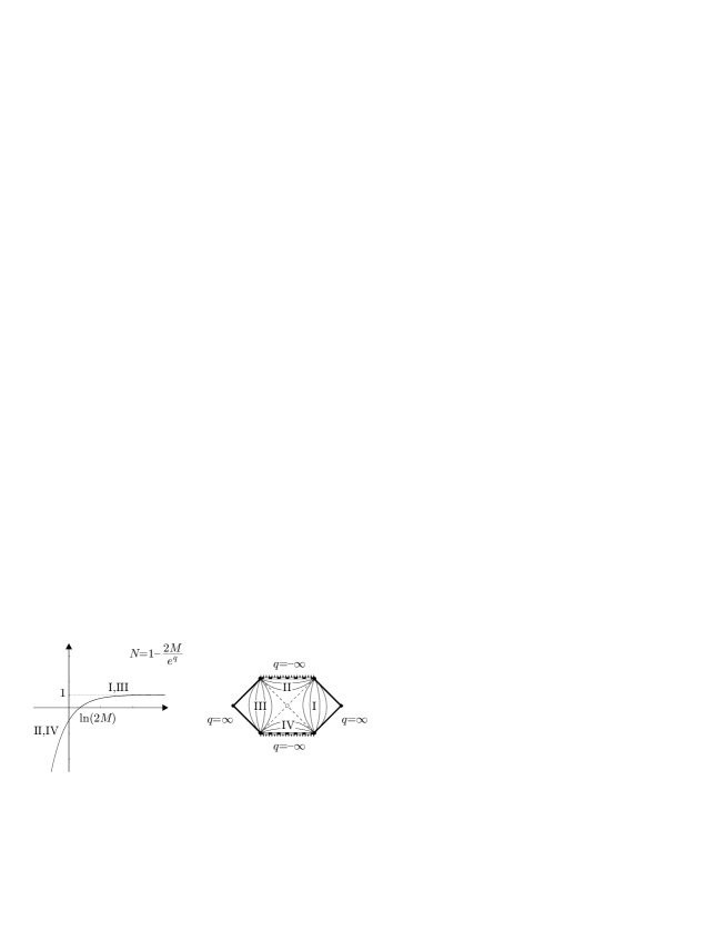
Figure 7: The conformal factor and the global solution for two-dimensional dilaton gravity. The singularity at $q=-\infty$ is complete for light like extremals and incomplete for time like ones.

The exponential behaviour of the conformal factor (52) near the curvature singularity when $q\rightarrow-\infty$ leads to qualitative distinction of this solution from the black hole because the singularity is semi complete. Namely, all light like extremals approach the singularity at an infinite value of the canonical parameter while time and space like extremals meet the singularity at a finite value [10].

Note that the dilaton gravity is locally equivalent to quadratic two-dimensional gravity with torsion but global equivalence is abcent [9].

6.6 Minkowskian plain

The above examples demonstrate the rules of construction of global Lorentz surfaces of nonconstant curvature. The following two examples show how the rules work for constant curvature surfaces, the classical field of differential geometry. Example of the Minkowskian plain is also important because it will be used later in the proof of the smoothness of global solutions in saddle points.

For the Minkowskian plain the scalar curvature is equal to zero, and the conformal factor is a linear function

$$N=bq+c,~{}~{}~{}~{}~{}~{}b,c={\sf const}.$$ (53)

There are two qualitatively different cases $b=0$ and $b\neq 0$.

For $b=0$ the metric (1) is the Minkowskian one

$$ds^{2}=c(d\tau^{2}-d\sigma^{2}),$$ (54)

where we assume $c>0$ for definiteness. The conformal factor $N=c$ does not have nor singularities nor zeroes. Then equation (2) yeilds

$$q=\pm c\sigma.$$

Here the $\pm$ sign corresponds to different orientation of the variable $q$ with respect to space coordinate. Since this variable does not enter the metric, it can be excluded from the consideration. Hence one square conformal block shown in Fig. 8 corresponds to the interval $q\in(-\infty,\infty)$.

Figure 8: Two representations of the Minkowskian plain in the absence and presence of one horizon. In the last case the Minkowskian plain is sewed from four conformal blocks.

Let us consider nonzero $b>0$. Then the conformal factor (53) has one simple zero at $q_{1}=-c/b$. Two pairs of conformal blocks correspond to the intervals $(-\infty,q_{1})$ and $(q_{1},\infty)$ wich are sewed together along horizons as shown in Fig. 8. Let us show how this solution is related to the previous representation of the Minkowskian plain by one conformal block. Without loss of generality we set $c=0$, that is

$$ds^{2}=b|q|(d\tau^{2}-d\sigma^{2})$$ (55)

This can be always achieved by the shift $q\rightarrow q+{\sf const}$, which does not affect the global structure of the solution. Consider all four domains

Domain I. For $N=bq$ equation (2) yeilds

$$q=e^{b\sigma}$$ (56)

up to a shift of $\sigma$. Corresponding metric is static, has the form

$$ds^{2}=be^{b\sigma}(d\tau^{2}-d\sigma^{2}),~{}~{}~{}~{}~{}~{}\tau,\sigma\in{\mathbb{R}}^{2},$$ (57)

and is defined on the whole plain $\tau,\sigma\in(-\infty,\infty)$. Transition to the light cone coordinates (25) and the conformal transformation

$$u=\frac{2}{b}e^{\frac{b\xi}{2}}>0,~{}~{}~{}~{}~{}~{}v=-\frac{2}{b}e^{-\frac{b\eta}{2}}<0$$ (58)

yield the Minkowskian metric

$$ds^{2}=b\,dudv,$$ (59)

defined on the first quadrant.

Domain III. For the variable $q$ and the metric one has

$$q = e^{-b\sigma},$$ (60)

$$ds^{2} = be^{-b\sigma}(d\tau^{2}-d\sigma^{2}),~{}~{}~{}~{}~{}~{}\tau,\sigma\in{\mathbb{R}}^{2}.$$ (61)

The conformal transformation leading to the Minkowskian metric (59) has the form

$$u=-\frac{2}{b}e^{-\frac{b\xi}{2}}<0,~{}~{}~{}~{}~{}~{}v=\frac{2}{b}e^{\frac{b\eta}{2}}>0,$$ (62)

corresponding to the third quadrant.

Domain II. This domain is homogeneous

$$q = -e^{b\tau},$$ (63)

$$ds^{2} = be^{b\tau}(d\tau^{2}-d\sigma^{2}),~{}~{}~{}~{}~{}~{}\tau,\sigma\in{\mathbb{R}}^{2}.$$ (64)

The conformal transformation yielding the Minkowskian metric has the form

$$u=\frac{2}{b}e^{\frac{b\xi}{2}}>0,~{}~{}~{}~{}~{}~{}v=\frac{2}{b}e^{\frac{b\eta}{2}}>0,$$ (65)

corresponding to the second quadrant.

Domain IV. Analogously, for the variable $q$ and the metric one has

$$q = -e^{-b\tau},$$ (66)

$$ds^{2} = be^{-b\tau}(d\tau^{2}-d\sigma^{2}),~{}~{}~{}~{}~{}~{}\tau,\sigma\in{\mathbb{R}}^{2}.$$ (67)

The conformal transformation leading to the Minkowskian metric is

$$u=-\frac{2}{b}e^{-\frac{b\xi}{2}}<0,~{}~{}~{}~{}~{}~{}v=-\frac{2}{b}e^{-\frac{b\eta}{2}}<0,$$ (68)

corresponding to the fourth quadrant.

For all four domains the horizon $q_{1}=0$ corresponds to the coordinate axes $u=0$ and $v=0$. Simple calculations show that in all domains

$$q=-\frac{b^{2}}{4}(t^{2}-x^{2}),$$ (69)

where

$$u=t+x,~{}~{}~{}~{}~{}~{}v=t-x.$$

These coordinates yeild the simplest example of the Kruskal–Szekeres coordinates for the metric (55). That is the variable $q$ is the hyperbolic radius of the polar coordinate system on the Minkowskian plain. For the hyperbolic polar angle in the static domains

$$\varphi={\sf arcth}\left(\frac{t}{x}\right),$$

one has

$${\rm I}:~{}~{}\varphi=\frac{b}{2}\tau,~{}~{}~{}~{}~{}~{}{\rm III}:~{}~{}\varphi=-\frac{b}{2}\tau.$$

In the homogeneous domains

$$\varphi={\sf arcth}\left(-\frac{x}{t}\right),$$

and

$${\rm II}:~{}~{}\varphi=-\frac{b}{2}\sigma,~{}~{}~{}~{}~{}~{}{\rm IV}:~{}~{}\varphi=\frac{b}{2}\sigma.$$

Hence conformal transformations (58), (62), (65), and (68) yield one and the same Minkowskian metric (59) in all four domains but defined on different quadrants, the smoothness of the metric on the horizons and the saddle point for the $q$ variable (69) is proved.

Thus the linear conformal factor (53) for $b\neq 0$ describes the Minkowskian plain, Fig. 8, b, in the hyperbolic coordinate system.

6.7 Constant curvature surfaces

Let us consider constant curvature surfaces for which the conformal factor is a quadratic polinomial (19). For definiteness we consider positive curvature surfaces $a>0$. Negative curvature surfaces are obtained from the positive curvature ones by the transformation $\tau\leftrightarrow\sigma$, that is by the rotation all the diagrams by the angle $\pi/2$. Depending on the values of the constants $a,b,c$ equation $N(q)=0$ may not have, have one or two zeroes. Consider all three cases leading to different metrics and Carter–Penrose diagrams for the constant curvature surfaces consequtively. Without loss of generality we set $b=0$, which can be always achieved by the shift of $q$.

Absence of a horizon.

$$N=-(aq^{2}+c),~{}~{}~{}~{}~{}~{}a>0,~{}c>0.$$ (70)

Since $N<0$ and singularities and zeroes are absent, the global solution corresponds to an infinite interval $q\in(-\infty,\infty)$. It is represented by the homogeneous conformal block of type II or IV shown in Fig. 9.

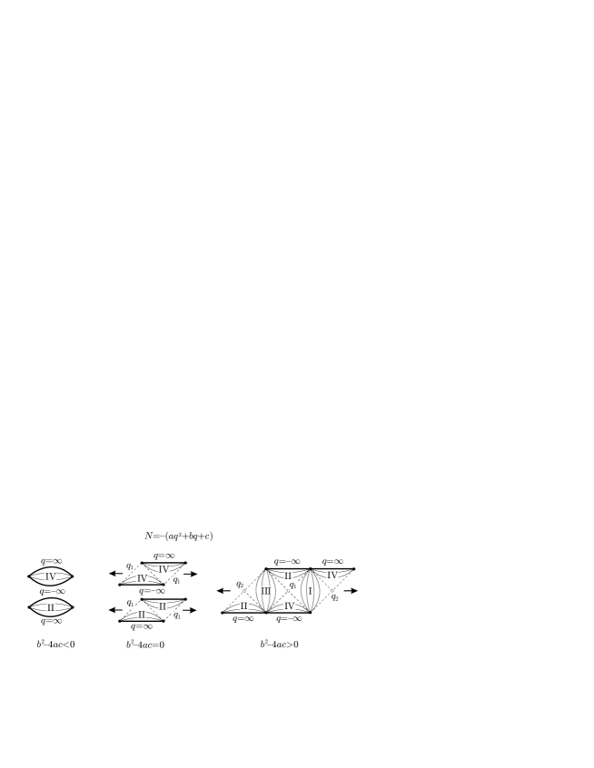
Figure 9: Carter–Penrose diagrams for constant positive curvature surfaces. There are three cases: the absence of a horizon, the existence of one or two horizons.

In the domain IV equation (2) for the conformal factor (70) yeilds

$$q=\sqrt{\frac{c}{a}}\,{\sf tg}(\sqrt{ac}\,\tau)$$ (71)

up to a shift of $\tau$. Time coordinate varies in the finite interval

$$-\frac{\pi}{2}<\sqrt{ac}\,\tau<\frac{\pi}{2},$$

corresponding to a lens type diagram. The metric in the $\tau,\sigma$ plain has the form

$$ds^{2}=\frac{c}{{\sf cos}^{2}(\sqrt{ac}\,\tau)}(d\tau^{2}-d\sigma^{2}).$$ (72)

This metric is a global one and defined on the whole universal covering space of constant curvature. In the domain II the metric has the same form except the orientation of $q$ with respect to $\tau$ changes.

One horizon.

$$N=-aq^{2},~{}~{}~{}~{}~{}~{}a>0.$$ (73)

At the point $q_{1}=0$ the conformal factor has a zero of second order corresponding to a horizon. In domain IV for both intervals $q\in(-\infty,0)$ and $q\in(0,\infty)$ one has

$$q = -\frac{1}{a\tau},$$ (74)

$$ds^{2} = \frac{1}{a\tau^{2}}(d\tau^{2}-d\sigma^{2}).$$ (75)

In this case the fundamenral region consists of two triangular conformal blocks shown in Fig. 9,b. To get the universal covering space diffeomorphic to the diagram of lens type from the previous case the fundamental domain should be extended in both directions. Identifying left and right boundary of the fundamental domain one gets the surface diffeomorphic to the one sheet hyperboloid (see, for example, [6]).

Two horizons.

$$N=-(aq^{2}+c),~{}~{}~{}~{}~{}~{}a>0,~{}c<0.$$ (76)

This conformal factor has two simple zeroes at the points $q_{1,2}=\mp\sqrt{-c/a}$. Hence there are six conformal blocks for three intervals. The symmetry of the conformal factor imply that four homogeneous and two static conformal blocks are essentially the same. For a homogeneous domain IV one has

$$q = -\sqrt{-\frac{c}{a}}\,{\sf cth}(\sqrt{-ac}\,\tau),$$ (77)

$$ds^{2} = \frac{-c}{{\sf sh}^{2}(\sqrt{-ac}\,\tau)}(d\tau^{2}-d\sigma^{2}).$$ (78)

For static domain I one has

$$q = \sqrt{-\frac{c}{a}}\,{\sf th}(\sqrt{-ac}\,\sigma),$$ (79)

$$ds^{2} = \frac{-c}{{\sf ch}^{2}(\sqrt{-ac}\,\sigma)}(d\tau^{2}-d\sigma^{2}).$$ (80)

Different forms of the metric on a constant curvature surface are caused by different coordinate choices. Since all metrics are conformally flat they are related by conformal coordinate transformations. Let us write metric (75) in light cone coordinates (25) and make a conformal transformation $\xi\rightarrow u(\xi)$, $\eta\rightarrow v(\eta)$, then

$$ds^{2}=\frac{1}{a\tau^{2}}(d\tau^{2}-d\sigma^{2})=\frac{4}{a(\xi+\eta)^{2}}\frac{d\xi}{du}\frac{d\eta}{dv}dudv.$$ (81)

The transformation

$$\xi=\frac{2}{\sqrt{ac}}{\sf tg}\left(\frac{\sqrt{ac}}{2}u\right),~{}~{}~{}~{}~{}~{}\eta=-\frac{2}{\sqrt{ac}}{\sf ctg}\left(\frac{\sqrt{ac}}{2}v\right)$$ (82)

yields the metric (75). Transformations

$$\xi=\frac{2}{\sqrt{-ac}}{\sf th}\left(\frac{\sqrt{-ac}}{2}u\right),~{}~{}~{}~{}~{}~{}\eta=\frac{2}{\sqrt{-ac}}{\sf th}\left(\frac{\sqrt{-ac}}{2}v\right)$$ (83)

and

$$\xi=\frac{2}{\sqrt{-ac}}{\sf th}\left(\frac{\sqrt{-ac}}{2}u\right),~{}~{}~{}~{}~{}~{}\eta=-\frac{2}{\sqrt{-ac}}{\sf cth}\left(\frac{\sqrt{-ac}}{2}v\right)$$ (84)

yeild metrics (78) and (80), respectively.

7 Eddington–Finkelstein coordinates

The smoothness of the metric on horizons is proved by writing it in a new coordinate system covering horizons. Let the zero $q_{j}$ of an odd order be inside the interval $(q_{-},q_{+})$. For definiteness we assume that the conformal factor is positive and negative in the adjacent intervals $(q_{j-1},q_{j})$ and $(q_{j},q_{j+1})$, respectively. In accordance with the rule 4) the stationary conformal block I must be sewed together with two homogeneous blocks of types II and IV. Horizons can be covered by the Eddington–Finkelstein coordinates [18, 19], introduced in the following way.

Sewing together domains I–II. To prove the smoothness of the sewing together domains I and II by themselves and the metric on them the Eddington–Finkelstein coordinates will be introduced. These coordinates cover the chosen domains, the transition functions in each of the domain being in the ${\cal C}^{l+1}$ class, and the metric in new coordinates including horizons is in ${\cal C}^{l}$ class.

Let us go from the conformal coordinates $\tau,\sigma$ on the domain I to the Eddington–Finkelstein coordinates $\xi,q$

$$\tau=\xi-{\displaystyle\int^{q}\frac{dr}{N(r)}},~{}~{}~{}~{}~{}~{}\sigma={\displaystyle\int^{q}\frac{dr}{N(r)}}.$$ (85)

The last integral is divergent on horizons but this is not important because the transformation (85) is considered only in the interior points of the domain I. The transition functions are obviously of ${\cal C}^{l+1}$ class in the interior points. Substituting expressions for the differentials

$$d\tau=d\xi-\displaystyle{\frac{dq}{N}},~{}~{}~{}~{}~{}~{}d\sigma=\displaystyle{\frac{dq}{N}},$$ (86)

in the metric (27) one gets the quadratic form

$$ds^{2}=Nd\xi^{2}-2dqd\xi.$$ (87)

Determinant of this metric is equal to ${\sf det}g_{\alpha\beta}=-1$, and the metric (87) is defined for all $\xi\in(-\infty,\infty)$ and, importantly, for all $q\in(q_{-},q_{+})$ and not only for $q\in(q_{j-1},q_{j})$. That is the metric (87) is defined in a larger domain then the starting one (1). The smoothness of the metric (87) coinsides with the smothness of the conformal factor everywhere including horizons.

In the homogeneous domain of the type

$$\text{II}:~{}~{}ds^{2}=-N(q)(d\tau^{2}-d\sigma^{2}),~{}~{}~{}~{}\frac{dq}{d\tau}=N(q)<0,$$ (88)

we go to the Eddington–Finkelstein coordinates

$$\tau={\displaystyle\int^{q}\frac{dr}{N}},~{}~{}~{}~{}~{}~{}\sigma=\xi-{\displaystyle\int^{q}\frac{dr}{N}}.$$ (89)

The coordinates transformation in the domain II differs from the transformation (85). However the metric (88) takes the form (87). This means that Eddington–Finkelstein coordinates with a given metric (87) isometrically cover domains I and II. This proves that the smoothness of the metric on the horizon coinsides with the smoothness of the conformal factor. One may check that the horizon $q_{j}$ is an extremal by itself in the Eddington–Finkelstein coordinates.

The domains III–IV can be sewed analogously. Explicit formulas for the transition to Eddington–Finkelstein coordinates have the form

$${\rm III}:~{}~{}~{}~{}~{}~{}\tau=\xi+{\displaystyle\int^{q}\frac{dr}{N(r)}},~{}~{}~{}~{}~{}~{}\sigma=-{\displaystyle\int^{q}\frac{dr}{N(r)}}.$$ (90)

and

$${\rm IV}:~{}~{}~{}~{}~{}~{}\tau=-{\displaystyle\int^{q}\frac{dr}{N}},~{}~{}~{}~{}~{}~{}\sigma=\xi+{\displaystyle\int^{q}\frac{dr}{N}}.$$ (91)

The metric has the same form in both domains

$$ds^{2}=Nd\xi^{2}+2dqd\xi.$$ (92)

Metrics (87) and (92) are connected between themselves by the transformation $\xi\rightarrow-\xi$.

Sewing together domains I–IV. In the domain I we choose the coordinates

$$\tau=\eta+{\displaystyle\int^{q}\frac{dr}{N(r)}},~{}~{}~{}~{}~{}~{}\sigma={\displaystyle\int^{q}\frac{dr}{N(r)}},$$ (93)

in which the metric takes the form

$$ds^{2}=Nd\eta^{2}+2dqd\eta.$$ (94)

The coordinates

$$\tau=-{\displaystyle\int^{q}\frac{dr}{N(r)}},~{}~{}~{}~{}~{}~{}\sigma=-\eta-{\displaystyle\int^{q}\frac{dr}{N(r)}}$$ (95)

yield the same metric in the domain IV.

Similar coordinates are introduced for sewing together the domains II and III, the corresponding metric being related to the metric (94) by the transformation $\eta\rightarrow-\eta$.

If the horizon $q_{j}$ has even degree and in both intervals $(q_{j-1},q_{j})$ and $(q_{j},q_{j+1})$ and the conformal factor is, for example, positive, then according to the rule 4) the blocks of one type are only sewed together. To prove the smoothness of the sewing on the blocks of type I and III the coordinates (85) and (90) are introduced respectively.

Thus the smoothness of the metric and, consequently, Christoffel’s symbols and curvature tensor is proved on all horizons. Metric in the Eddington–Finkelstein coordinates (87) covers the whole chain of the conformal blocks for $q\in(q_{-},q_{+})$ of types I and II for the fundamental domain. For this chain the coordinate $q$ decreases with the increasong of $\tau$. The chain is a ${\cal C}^{l+1}$ manifold because the transition functions (85), (89) are of this class. Metric (92) covers parallel chain of the conformal blocks III and IV. Metric in the form (94) covers a perpendicular chain of the conformal blocks I and IV. In the interior of every chain the metric in the Eddington–Finkelstein coordinates is nondegenerate and of the ${\cal C}^{l}$ class. The fundamental domain consists of two parallel chains of conformal blaocks. If there is at least one zero of odd degree inside the interval, then the fundamental domain is connected. In the opposite case one has two disconnected fundamental domains. This is the meaning of the rule 5).

The Eddington–Finkelstein coordinates are natural ones in the following sence. First of all note that the extension of the solution has to be performed along variable $q$ because it defines the completeness of the manifold and the curvature singularities, and it is a scalar function in addition. Since for a static solution the variable $q$ depends only on $\sigma$ the $q$ variable (85), (90), (93), may be chosen as a coordinate instead of $\sigma$, the coordinates being one to one related by the equation (2) up to an insignificant shift of $\sigma$ in each domain. After that the light cone coordinate (25) is introduced instead of the time coordinate. There are two possibilities, and both of them are realised yeilding coordinates on the two perpendicular chains of conformal blocks. The Eddington–Finkelstein coordinates on the homogeneous blocks are introduced analogously. One may check that there is no possibility to sew together the domains I, III or II, IV. Moreover straightforward calculations prove that the derivatives of $q$ are discontinuos under this sewing while $q$ by itself is a continuous function [6].

8 Smoothness of the metric in the saddle point

The Eddington–Finkelstein coordinates do not cover the saddle points been situated on the horizons crossing. Saddle points correspond to zeroes of $N(q)$ situated at finite points with the exponent $m=1$ or $m\geq 2$ (see Fig. 3). If the point $q_{j}$ is a zero of second order or higher then the saddle point is complete and nothing has to be proved. If the point $q_{j}$ is a simple zero then one may introduce coordinates covering a neiborhood of the saddle point. Since the behaviour of the conformal factor near the zero is the same as for the Minkowskian plain we go to the Kruskal–Szekeres coordinates with $b=N^{\prime}(q_{j})$ (see section 6.6). Explicit transformation formulas in domains I–IV have the form (58), (65), (62), and (68), respectively. As for the Minkowskian plain the $u,v$ coordinates cover a neighborhood of the saddle point including the domains of all four types sewed together along horizons. In all four quadrants metric (1) takes the same form

$$ds^{2}=|N|{\sf exp}\left(-\int^{q}dp\frac{N^{\prime}(q_{j})}{N(p)}\right)\,dudv={\sf exp}\left(\int^{q}dp\frac{N^{\prime}(p)-N^{\prime}(q_{j})}{N(p)}\right)\,dudv.$$ (96)

Since the limit of the integrand exists in the saddle point the integral is a smooth function. This proves nondegeneracy and smoothness of the metric in the saddle point, the differentiability of the metric being the same as of the conformal factor. The Kruskal–Szekeres coordinates can be obviously introduced near every saddle point of first order. Because the transition functions to the Kruskal–Szekeres coordinates are of ${\cal C}^{\infty}$ class, then the ${\cal C}^{l+1}$ smoothness class of the universal covering space is defined by the transition functions to the Eddington–Finkelstein coordinates. This finishes the proof of the main theorem 2.

9 Conclusion

The method of building of global solutions for two-dimensional metrics of Lorentz signature considered in the present paper is simple and constructive. If the gravity equations of motion lead to the metric (1) with some conformal factor then it is sufficient to analyse its zeroes and singularities. Afterwards the universal covering space is uniquely constructed. All other global solutions are factor spaces of the universal covering space under the action of free and descrete transformation group. The possibilities to construct solutions with nontrivial fundamental groups by the identification of the boundary of the fundamental domain are noted in the paper. In a general case the finding of descrete transformation groups depends on the form of the conformal factor and is the subject of independent investigation.

The author is very gratefull to T. Klösch, W. Kummer, T. Strobl, I. V. Volovich, V. V. Zharinov for fruitfull discussions on the subject and the Russian Fund for basic research, grants RFBR-99-01-00866 and RFBR-96-15-96131 for financial support.

References

- [1] Kruskal M. D. Maximal extension of Schwarzschild metric // Phys. Rev. 1960. V. 119, N 5. P. 1743–1745.
- [2] Szekeres G. On the singularities of a riemannian manifold // Publ. Mat. Debrecen. 1960. V. 7, N 1–4. P. 285–301.
- [3] Schwarzschild K. Über das Gravitationssfeldeines Massenpunktes nach der Einsteinschen Theorie // Sitzungsber. Akad. Wiss. Berlin. 1916. P. 189–196.
- [4] Bogolubov N. N. On sone ergodic properties of the indecomposable transformation groups // Naukovi zapiski KDU im. T. G. Shevchenka. Fiziko-matematichny zbirnik. 1939. V. 4, N 5. P. 45–52. [In Ukrainian].
- [5] Carter B. Black hole equilibrium states // In C. DeWitt and B. C. DeWitt, editors, Black Holes, pages 58–214, New York, 1973. Gordon & Breach.
- [6] Katanaev M. O. All universal coverings of two-dimensional gravity with torsion // J. Math. Phys. 1993. V. 34, N 2. P. 700–736.
- [7] Katanaev M. O., Volovich I. V. String model with dynamical geometry and torsion // Phys. Lett. 1986. V. 175B, N 4. P. 413–416.
- [8] Klösch T., Strobl T. Classical and quantum gravity in dimensions: II. The universal coverings // Class. Quantum Grav. 1996. V. 13. P. 2395–2421.
- [9] Katanaev M. O., Kummer W., Liebl H. Geometric interpretation and classification of global solutions in generalized dilaton gravity // Phys. Rev. 1996. V. D53, N 10. P. 5609–5618.
- [10] Katanaev M. O., Kummer W., Liebl H. On the completeness of the black hole singularity in 2d dilaton theories // Nucl. Phys. 1997. V. B486. P. 353–370.
- [11] Katanaev M. O., Klösch T., Kummer W. Global properties of warped solutions in general relativity // gr-qc/9807079, 35 pp. Ann. Phys. .
- [12] B. A. Dubrovin, S. P. Novikov, and A. T. Fomenko. Contemporary geometry. Nauka, Moscow, fourth edition, 1998. [In Russian].
- [13] L. D. Landau and E. M. Lifshitz. The Classical Theory of Fields. Pergamon, New York, second edition, 1962.
- [14] M. O. Katanaev. New integrable model: two-dimensional gravity with dynamical torsion. Sov. Phys. Dokl., 34:982–983, 1989.
- [15] Katanaev M. O. Complete integrability of two-dimensional gravity with dynamical torsion // J. Math. Phys. 1990. V. 31, N 4. P. 882–891.
- [16] Witten E. String theory and black holes // Phys. Rev. 1991. V. D44, N 2. P. 314–324.
- [17] Mandal G., Sengupta A. M., Wadia S. R. Classical solutions of two-dimensional string theory // Mod. Phys. Lett. 1991. V. 6. P. 1685–1692.
- [18] Eddington A. S. A comparison of Whitehead’s and Einstein’s formulae // Nature. 1924. V. 113. P. 192.
- [19] Finkelstein D. Past-future asymmetry of the gravitational field of a point particle // Phys. Rev. 1958. V. 110, N 4. P. 965–967.