Influence of scalar fields on the approach to a cosmological singularity

Abstract

The method of consistent potentials is used to explain how a minimally coupled (classical) scalar field can suppress Mixmaster oscillations in the approach to the singularity of generic cosmological spacetimes.

98.80.Dr, 04.20.J

In their long-term study of the approach to the singularity in generic cosmological spacetimes [1, 2, 3, 4, 5], Belinskii, Khalatnikov, and Lifshitz (BKL) concluded that generic cosmological spacetimes approach the singularity as a (different) Mixmaster universe [6] at every spatial point. The Mixmaster universe is characterized by “oscillations” from one Kasner solution [7] to another. When BKL considered the influence of a classical minimally coupled scalar field on the approach to the singularity, they found that it can suppress Mixmaster oscillations [8]. While this result is now well-known, the mechanism by which it happens is not widely appreciated. I wish to address this issue here.

The role of the scalar field may be easily clarified using the method of consistent potentials (MCP) originally due to Grubis̆ić and Moncrief [9]. The MCP has been applied to a variety of cosmological spacetimes to explain the nature of the (numerically observed) approach to the singularity in spatially inhomogeneous cosmologies [10]. The MCP first assumes that the approach to the singularity is asymptotically velocity term dominated (AVTD) [11] and then looks for a contradiction. If the model is AVTD, it approaches arbitrarily closely to a Kasner solution with a possibly different Kasner solution at every spatial point. For any model, an asymptotic velocity term dominated (VTD) solution may be found by neglecting all terms in Einstein’s equations containing spatial derivatives and taking the limit as $\tau\to\infty$. (The MCP includes the implicit assumption that strong cosmic censorship holds for these cosmological models — i.e. there exists a foliation labeled by $\tau$ such that some curvature invariant blows up as $\tau\to\infty$.) If the model is actually AVTD, then substitution of the VTD solution into the full Einstein equations will be consistent — asymptotically, all terms neglected in obtaining the VTD solution will be exponentially small. For convenience, the MCP will be applied to the Hamiltonian whose variation yields the relevant Einstein equations since exponentially small (growing) terms in the Hamiltonian will yield exponentially small (growing) terms in Einstein’s equations upon variation. Any terms which cannot be made consistent with the VTD solution indicate, within the MCP, that the model is not AVTD. Here I shall consider essentially the same models as in [10] but with the addition of a scalar field. I shall explore the influence of a massless, minimally coupled scalar field in some detail. The possibly interesting dynamics which may result from exponentially coupled scalar fields will be discussed elsewhere. For each cosmology, I shall use the MCP to show how the scalar field yields an asymptotically velocity term dominated (AVTD) approach to the singularity.

Consider first the primary Mixmaster model — the spatially homogeneous vacuum Bianchi Type IX cosmology [4, 6]. In the presence of a spatially homogeneous scalar field, $\phi(\tau)$, Einstein’s equations are obtained from the variation of the Hamiltonian constraint ${\cal H}=0$ where

$$2{\cal H}=-p_{\Omega}^{2}+p_{+}^{2}+p_{-}^{2}+p_{\phi}^{2}+V(\Omega,\beta_{\pm})+e^{6\Omega}{\cal V}(\phi)\ .$$ (1)

In Eq. (1), $\Omega$ is $1/3$ the logarithm of the spatial volume and $\beta_{\pm}$ the anisotropic shears with $p_{\Omega}$ and $p_{\pm}$ their conjugate momenta. The scalar field momentum, $p_{\phi}$, plays a crucial role in the approach to the singularity. The spatial scalar curvature appears in $V(\Omega,\beta_{\pm})={}^{3}\/g\,{}^{3}\/R$ for ${}^{3}\/g$ and ${}^{3}\/R$ respectively the determinant and scalar curvature of the spatial metric while ${\cal V}(\phi)$ is the scalar field potential. The key to the influence of the scalar field is the additional kinetic term in Eq. (1). Any scalar field coupling which produces such a term will yield the same effect as long as ${\cal V}(\phi)$ does not contain terms exponential in $\phi$. Let us consider

$${\cal H}={\cal H}_{K}+{\cal H}_{V}$$ (2)

where ${\cal H}_{K}$ contains all the momenta and

$$2{\cal H}_{V}= e^{4\Omega-8\beta_{+}}+e^{4\Omega+4\beta_{+}+4\sqrt{3}\beta_{-}}+e^{4\Omega+4\beta_{+}-4\sqrt{3}\beta_{-}}$$ (4)

$$-2(e^{4\Omega+4\beta_{+}}+e^{4\Omega-2\beta_{+}-2\sqrt{3}\beta_{-}}+e^{4\Omega-2\beta_{+}+2\sqrt{3}\beta_{-}})+e^{6\Omega}{\cal V}(\phi).$$

First, we note that, in these variables, the (strong curvature) singularity in these models occurs as $\Omega\to-\infty$. Thus, unless ${\cal V}(\phi)$ contains terms which asymptotically depend exponentially on $\Omega$ (through asymptotic linear dependence of $\phi$ on $\Omega$), $e^{6\Omega}{\cal V}(\phi)\to 0$ as $\Omega\to-\infty$. For now, we shall ignore this term.

The MCP requires us to assume that ${\cal H}={\cal H}_{K}$. Variation of this Hamiltonian yields equations with the solution

$$\beta_{\pm}=\beta_{\pm}^{0}+v_{\pm}|\Omega|,$$ (5)

$$\phi=\phi^{0}+v_{\phi}|\Omega|$$ (6)

where $v_{\pm}=p_{\pm}/|p_{\Omega}|$ and $v_{\phi}=p_{\phi}/|p_{\Omega}|$ with the momenta all constant. The Hamiltonian constraint ${\cal H}=0$ becomes ${\cal H}_{K}=0$ or

$$v_{+}^{2}+v_{-}^{2}+v_{\phi}^{2}=1.$$ (7)

First consider the vacuum case — $\phi\equiv 0$. Then we can write $v_{\pm}$ in polar coordinates (with unit radius) in the anisotropy plane. The minisuperspace (MSS) potential $V$ is dominated by the first three terms on the rhs of Eq. (4) so that

$$2V\approx e^{4\Omega-8\beta_{+}}+e^{4\Omega+4\beta_{+}+4\sqrt{3}\beta_{-}}+e^{4\Omega+4\beta_{+}-4\sqrt{3}\beta_{-}}.$$ (8)

Substitution of (5), with $v_{+}=\cos\theta$, $v_{-}=\sin\theta$, into (8) yields

$$2V\approx e^{-4|\Omega|(1+2\cos\theta)}+e^{-4|\Omega|(1-\cos\theta-\sqrt{3}\sin\theta)}+e^{-4|\Omega|(1-\cos\theta+\sqrt{3}\sin\theta)}.$$ (9)

Except for (the set of measure zero) $\theta=\{0,2\pi/3,4\pi/3\}$, any (generic) value of $\theta$ will cause one of the terms on the rhs of (9) to grow. For example, $1+2\cos\theta<0$ will cause the first term to grow. This condition arises for $\cos\theta<-1/2$ or $-2\pi/3<\theta<2\pi/3$.

With the addition of the scalar field, $v_{\phi}^{2}>0$, so that

$$v_{+}^{2}+v_{-}^{2}=1-v_{\phi}^{2}<1.$$ (10)

No term in Eq. (9) will grow if we can satisfy simulatneously with Eq. (10)

$$1+2v_{+} > 0,$$ (11)

$$1-v_{+}-\sqrt{3}v_{-} > 0,$$ (12)

$$1-v_{+}+\sqrt{3}v_{-} > 0.$$ (13)

Since $v_{+}^{2}+v_{-}^{2}=1$ is no longer required, solution of Eqs. (11) is possible if $v_{+}^{2}<1/2$ and $v_{-}^{2}<1/12$ which can occur if $2/3<v_{\phi}^{2}<1$. Since $p_{\Omega}>0$ decreases at each bounce [12], any initial value of $p_{\phi}$ will eventually yield $v_{\phi}^{2}>2/3$.

In the absence of the scalar field, the growing term in Eq. (9) causes a “bounce” (see [10]) which changes the values of $v_{\pm}$ according to the prescription first given by BKL [4]. If the new values of $v_{\pm}$ satisfy (11), there will be no further bounces so that the solution will approach (5)-(6). We see, then, that the main function of the scalar field is to weaken the restriction imposed by the Hamiltonian constraint on the gravitational “kinetic energy.” In Fig. 1, trajectories with and without the scalar field are shown in the $v_{+}$-$v_{-}$ plane. In the vacuum case, away from bounces, the trajectory must fall on the “Kasner circle” defined by $v_{+}^{2}+v_{-}^{2}=1$. For a small initial value of $p_{\phi}$, the non-vacuum model closely tracks the other until the amplitude of $v_{\phi}$ grows sufficiently large. At this point, the trajectory deviates noticeably from the Kasner circle. Shortly thereafter, $v_{\pm}$ are able to satisfy (11) so there are no more bounces and the values of $v_{\pm}$ no longer change. (This causes the trajectory in the $v_{\pm}$-plane to end.)

It is possible to retain the Mixmaster (oscillatory) behavior if ${\cal V}(\phi)$ in (1) is such that

$$e^{6\Omega}{\cal V}(\phi)=a^{2}e^{\alpha\phi}+b^{2}e^{-\zeta\phi}$$ (14)

where $\alpha,\ \zeta>0$. A potential of this type will, according to the MCP, yield an exponentially growing term in (4) unless $v_{\phi}=0$. But $v_{\phi}=0$ means that the usual Mixmaster oscillations will occur. Thus, given (14), there will be no way to avoid oscillations. Coupling between scalar field and gravitational degrees of freedom in $e^{6\Omega}\,{\cal V}(\phi)$ could lead to very complicated behavior. BKL, in fact, by coupling an electromagnetic field to a Brans-Dicke-like scalar field so as to produce a potential term like (14) where $a$ and $b$ are functions of the electromagnetic field, claimed to have restored the oscillations suppressed initially by the scalar field alone [8]. Potentials exponential in the scalar field can also arise in string theory [13].

The most complicated models to which the MCP has been applied are vacuum cosmologies with a single spatial $U(1)$ symmetry and $T^{3}$ spatial topology [14, 15, 16, 17, 10]. The degrees of freedom are $\{x,z,\Lambda,\varphi,\omega\}$ with conjugate momenta $\{p_{x},p_{z},p_{\Lambda},p,r\}$. The variables are functions of spatial coordinates $u$ and $v$ and time $\tau$. Here the Hamiltonian constraint (${\cal H}=0$) is

$${\cal H} = {1\over 8}p_{z}^{2}+{1\over 2}e^{4z}p_{x}^{2}+{1\over 8}p^{2}+{1\over 2}e^{4\varphi}r^{2}-{1\over 2}p_{\Lambda}^{2}$$ (17)

$$+\left({e^{\Lambda}e^{ab}}\right),_{ab}-\left({e^{\Lambda}e^{ab}}\right),_{a}\Lambda,_{b}+e^{\Lambda}\left[\left({e^{-2z}}\right),_{u}x,_{v}-\left({e^{-2z}}\right),_{v}x,_{u}\right]$$

$$+2e^{\Lambda}e^{ab}\varphi,_{a}\varphi,_{b}+{1\over 2}e^{\Lambda}e^{-4\varphi}e^{ab}\omega,_{a}\omega,_{b}$$

$$= {\cal H}_{K}+\,{\cal H}_{V}$$ (18)

where ${\cal H}_{K}$ contains only momenta and

$$e^{ab}={1\over 2}e^{-2z}\left({\matrix{{e^{4z}+(1-x)^{2}}&{-e^{4z}+(1-x^{2})}\cr\cr{-e^{4z}+(1-x^{2})}&{e^{4z}+(1+x)^{2}}\cr}}\right)\,.$$ (19)

Its variation yields Einstein’s equations. A transformation $\Lambda\to\Lambda-2\tau$ will restore the explicit time dependence in (17) found in [15, 16, 17]. To apply the MCP, the appropriate generalization of (5) is required. This is found by solving the velocity term dominated (VTD) equations obtained by neglecting all terms in Einstein’s equations containing spatial derivatives. In the limit as $\tau\to\infty$, we find [16]

$$z = -v_{z}\tau,\quad x=x_{0},\quad p_{z}=-4v_{z},\quad p_{x}=p_{x}^{0},\quad\varphi=-v_{\varphi}\tau,$$ (20)

$$\omega = \omega_{0},\quad p=-4v_{\varphi},\quad r=r^{0},\quad\Lambda=\Lambda_{0}-v_{\Lambda}\tau,\quad p_{\Lambda}=v_{\Lambda}$$ (21)

where $v_{z}$, $v_{\varphi}$, $x_{0}$, $p_{x}^{0}$, $\omega_{0}$, $r^{0}$, $\Lambda_{0}$, and $v_{\Lambda}>0$ are functions of $u$ and $v$ but independent of $\tau$. (The sign of $v_{\Lambda}$ is fixed to ensure collapse.) In the $VTD$ limit, the Hamiltonian constraint (17) becomes

$$-{1\over 2}p_{\Lambda}^{2}+{1\over 8}p^{2}+{1\over 8}p_{z}^{2}=0.$$ (22)

To obtain this expression, it was necessary to assume $v_{\varphi}>0$ and $v_{z}>0$ so that the exponential terms containing $p_{x}^{2}\,e^{4z}$ and $r^{2}\,e^{4\varphi}$ in ${\cal H}_{K}$ would be exponentially small. However, $v_{\varphi}>0$ causes the term ${1\over 2}e^{\Lambda-4\varphi}e^{ab}\nabla_{a}\omega\nabla_{b}\omega$ in (17) to grow unless

$$\mathop{\lim}\limits_{\tau\to\infty}\,(\Lambda-2z-4\varphi),_{\tau}=-v_{\Lambda}+2v_{z}+4v_{\varphi}<0.$$ (23)

This condition is obtained by noting that $v_{z}>0$ implies $z\to-\infty$ as $\tau\to\infty$ so that $e^{ab}$ from (19) behaves as $e^{-2z}$. As was shown in [16, 17], the VTD form of the Hamiltonian constraint (22) gives $v_{\Lambda}^{2}=4v_{z}^{2}+4v_{\varphi}^{2}$ so that (23) cannot be satisfied with $v_{\varphi}>0$ and $v_{z}>0$. On the other hand, if either of these is $<0$, either $r^{2}e^{4\varphi}$ or $p_{x}^{2}e^{4z}$ in (17) will grow. This leads to the prediciton (observed numerically) that the approach to the singularity is oscillatory.

Just as in the spatially homogeneous case, in the presence of a scalar field $\phi(u,v,\tau)$, the AVTD limit of the Hamiltonian constraint becomes

$$0=-{1\over 2}p_{\Lambda}^{2}+{1\over 8}p^{2}+{1\over 8}p_{z}^{2}+{1\over 2}p_{\phi}^{2}$$ (24)

where $p_{\phi}$ is the scalar field momentum. It is now possible to simultaneously satisfy $v_{\varphi}>0$, $v_{z}>0$, and $-v_{\Lambda}+2v_{z}+4v_{\varphi}<0$ since $v_{\Lambda}^{2}=4v_{z}^{2}+4v_{\varphi}^{2}+p_{\phi}^{2}$ from (24) can be made arbitrarily large with a sufficiently strong scalar field. At any representative spatial point, after some number of oscillations, the momenta will move into the range needed to make the remaining evolution AVTD at that point. Presumably, as $\tau\to\infty$, the model will become AVTD almost everywhere.

It is possible to display this effect in a computer simulation of the full Einstein equations for $U(1)$ symmetric cosmologies with and without a scalar field. For convenience, $p_{\phi}$ is chosen to be constant in space. In Fig. 2, the evolution of $\varphi$ toward the singularity at three representative spatial points is shown for both cases. It is clear that the scalar field suppresses the oscillations. In Fig. 3, $\varphi(u=v,\tau)$ is shown for both cases. Note that the formation of ever smaller scale spatial structure is suppressed by the scalar field. Although these particular simulations can only be followed to $\tau\approx 40$, the MCP predicts that, for the scalar field model, at the spatial points of Figs. 2a and 2b, since $v_{\varphi}=0$ (to machine accuracy) and $v_{\varphi}>0$ respectively, no further bounces will occur. At the spatial point of Fig. 2c, at least one more bounce to change the sign of $v_{\varphi}$ is expected.

In models with two commuting spatial Killing fields, the Hamiltonian constraint enters in an interesting way. Consider the magnetic Gowdy model discussed in [18, 19]. Its variables $\{P,Q,\lambda\}$ and conjugate momenta $\{\pi_{P},\pi_{Q},\pi_{\lambda}\}$ depend on spatial coordinate $\theta$ and time $\tau$. Here, Einstein’s equations are obtained by variation of a Hamiltonian $H$ which is not the Hamiltonian constraint ${\cal H}$.

$$H={1\over{4\pi_{\lambda}}}\left[\pi_{P}^{2}+e^{-2P}\pi_{Q}^{2}+e^{-2\tau}\left(P,_{\theta}^{2}+e^{2P}Q,_{\theta}^{2}\right)\right]+B^{2}\pi_{\lambda}e^{(\lambda+\tau)/2}$$ (25)

where $B$ measures the strength of the magnetic field. The variation of (25) with respect to $\pi_{\lambda}$ yields

$$\lambda,_{\tau}=-{1\over{4\pi_{\lambda}^{2}}}\left[\pi_{P}^{2}+e^{-2P}\pi_{Q}^{2}+e^{-2\tau}\left(P,_{\theta}^{2}+e^{2P}Q,_{\theta}^{2}\right)\right]+B^{2}e^{(\lambda+\tau)/2}$$ (26)

which happens to be a rewriting of the Hamiltonian constraint ${\cal H}=0$. The AVTD solution obtained from the variation of (25) neglecting spatial derivatives is

$$P=v\,\tau,\quad\quad Q=Q_{0},\quad\quad\lambda=-v^{2}\,\tau$$ (27)

where $v=\mathop{\lim}\limits_{\tau\to\infty}\,\pi_{P}/(2\pi_{\lambda})$ depends on $\theta$ but not on $\tau$. As was described in [10], substitution of (27) into (25) shows that $V_{1}=e^{-2P}\pi_{Q}^{2}/\pi_{\lambda}$ will grow if $v<0$, $V_{2}=e^{2(P-\tau)}\,Q,_{\theta}^{2}/\pi_{\lambda}$ will grow if $v>1$ while $V_{3}=B^{2}e^{(\lambda+\tau)/2}$ will grow if $0<v<1$. Thus there is no value of $v$ consistent with the AVTD solution (27).

Now consider a scalar field with momentum $\pi_{\phi}$. Eq. (26) for $\lambda,_{\tau}$ gains an additional term and becomes

$$\lambda,_{\tau}=-{1\over 4}\left({{\pi_{P}}\over{\pi_{\lambda}}}\right)^{2}-{1\over 4}\,e^{-2P}\,\left({{\pi_{Q}}\over{\pi_{\lambda}}}\right)^{2}-{1\over 4}\left({{\pi_{\phi}}\over{\pi_{\lambda}}}\right)^{2}-{{e^{-2\tau}}\over{4\pi_{\lambda}^{2}}}\left(P,_{\theta}^{2}+e^{2P}Q,_{\theta}^{2}\right)+B^{2}e^{(\lambda+\tau)/2}$$ (28)

so that the AVTD solution is (since the equations for $P$ and $Q$ remain the same)

$$P=v\,\tau,\quad\quad Q=Q_{0},\quad\quad\lambda=-v^{2}\,\tau-v_{\phi}^{2}\,\tau$$ (29)

where $v_{\phi}=\pi_{\phi}/(2\pi_{\lambda})$. The magnetic potential will now grow if $0<v^{2}+v_{\phi}^{2}<1$. The additional scalar field kinetic energy means that we can have $0<v<1$ needed to keep $V_{1}$ and $V_{2}$ small with $v^{2}+v_{\phi}^{2}>1$ as is needed to keep $V_{3}$ small. Thus it is expected that, eventually, oscillations will cease as $v$ and $v_{\phi}$ enter the required ranges at almost every spatial point.

The results of numerical simulations of the magnetic Gowdy models (on $T^{3}$ rather than the solv-twisted torus [18]) with and without a scalar field are shown in Figures 4 and 5. In the former, the evolution toward the singularity of $P$ at three typical spatial points is shown. For the scalar field model, $v>0$ at all the spatial points so that no further oscillations are expected. Once again, the scalar field is seen to suppress the bounces and the growth of small-scale spatial structure. The entire evolution $P(\theta,\tau)$ is shown in Fig. 5. The larger the initial amplitude of $\pi_{\phi}$, the more quickly the bounces will be suppressed.

As in the spatially homogeneous case, the inhomogeneous models should continue to oscillate for scalar field potentials with an exponential form as in(14) almost everywhere. Although the mechanism described here has been examined only in particular systems using arguments based on the MCP approximation (reinforced by numerical simulations of the full equations), we expect the behavior discussed here to be valid generically. The bottom line is that the scalar field kinetic energy relaxes the restrictions imposed by the Hamiltonian constraint on the gravitational kinetic energy. Since it is these restrictions which lead to the Mixmaster oscillations, relaxing them will allow an AVTD approach to the singularity.

Figure Captions

Figure 1. Comparison of Bianchi IX MSS trajectories for models with (dashed line) and without (solid line) a scalar field. The Kasner circle is shown. Each saved data point of the scalar field model is shown with a dot. The code described in [12] is used to evolve spatially homogeneous Bianchi IX models. The initial scalar field momentum is $p_{\phi}=.001$. Both models start from the same initial data (a). At (b), it becomes clear that the scalar field model trajectory cannot reach the Kasner circle. The sequence of Kasner solutions (indicated by values of $v_{\pm}$) terminates at (c) for the scalar field model. The vacuum model continues indefinitely although only the first few bounces are shown. The trajectory first reaches (c) for $\log_{10}|\Omega|=3.45$.

Figure 2. Evolution of $\varphi$ toward the singularity for $U(1)$ symmetric vacuum (solid line) and scalar field (dashed line) models at representative spatial points. The scalar field is modeled by $p_{\phi}=5$ independent of space and time. The simulation consists of $128^{2}$ spatial grid points and is similar to those described in [17].

Figure 3. Evolution of $\varphi$ toward the singularity for $U(1)$ symmetric (a) vacuum and (b) scalar field models. A diagonal line $u=v$ in the $u$-$v$ plane is shown for the same simulation as in the previous figure with $0\leq u,v\leq 2\pi$ and $2\leq\tau\leq 39$.

Figure 4. Evolution of $P$ toward the singularity for a magnetic Gowdy model (see [18]) with (dashed line) and without (solid line) a scalar field. The initial scalar field momentum is $p_{\phi}=\cos\theta$. There are $1024$ spatial grid points in this simulation.

Figure 5. $P$ over the entire $\theta$-$\tau$ plane (a) without and (b) with a scalar field for the simulation of Figure 4 where $0\leq\theta-\theta_{0}\leq 2\pi$ for $\theta_{0}=-\pi/5$ and $0\leq\tau\leq 61$.

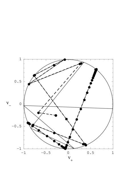
FIG. 1.:

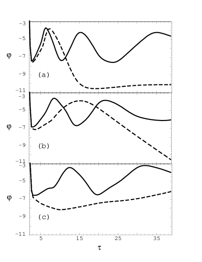
FIG. 2.:

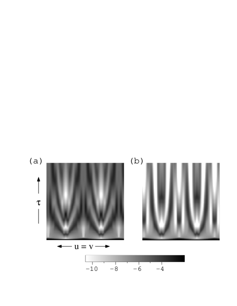
FIG. 3.:

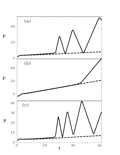
FIG. 4.:

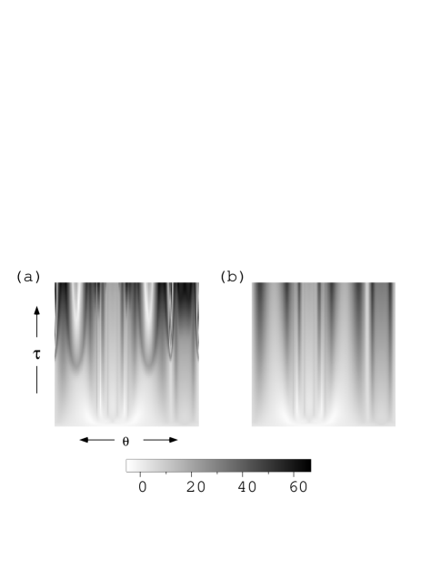
FIG. 5.:

REFERENCES

- [1] Belinskii, V. A. and Khalatnikov, I. M., Sov. Phys. JETP, 30, 1174–1180 (1969).
- [2] Belinskii, V. A. and Khalatnikov, I. M., Sov. Phys. JETP, 29, 911–917 (1969)
- [3] Belinskii, V. A. and Khalatnikov, I. M., Sov. Phys. JETP, 32, 169–172 (1971).
- [4] Belinskii, V. A., Lifshitz, E. M., and Khalatnikov, I. M., Sov. Phys. Usp. 13, 745 (1971).
- [5] Belinskii, V. A. and Khalatnikov, I. M. and Lifshitz, E. M., Adv. Phys., 31, 639–667 (1982).
- [6] C. W. Misner, Phys. Rev. Lett. 22, 1071 (1969).
- [7] Kasner, E., Trans. Am. Math. Soc., 27, 155–162, (1925).
- [8] Belinskii, V. A. and Khalatnikov, I. M., Sov. Phys. JETP, 36, 591–597 (1972).
- [9] Grubis̆ić, B. and Moncrief, V., Phys. Rev. D 47, 2371 (1993).
- [10] Berger, B. K., Garfinkle, D., Isenberg, J., Moncrief, V., Weaver, M., Mod. Phys. Lett., A13, 1565–1574 (1998).
- [11] Isenberg, J. A. and Moncrief, V., Ann. Phys. (N.Y.) 199, 84 (1990).
- [12] Berger, B. K., Garfinkle, D., and Strasser, E., Class. Quantum Grav., 14, L29–L36, (1997).
- [13] Løu, H. and Pope, C. N., Nucl.Phys., B465, 127–156 (1996).
- [14] Moncrief, V., Ann. Phys. (N.Y.), 167, 118, (1986).
- [15] Berger, B. K., and Moncrief, V., Phys. Rev. D, 48, 4676, (1993).
- [16] Berger, B. K. and Moncrief, V., Phys. Rev. D, 57, 7235–7240 (1998). Typographical errors appear in the full (but not asymptotic) VTD solutions given in Eq. (12) of this reference. The correct expressions are , , , .
- [17] Berger, B. K. and Moncrief, V., Phys. Rev. D, 58, 064023 (1998) .
- [18] Weaver, M., Isenberg, J., and Berger, B. K., Phys. Rev. Lett., 80, 2980 (1998).
- [19] M. Weaver, Ph.D. Thesis, U. of Oregon, 1999.