IFUP-TH 40/99

July 1999

Detection strategies for scalar gravitational

waves with interferometers and resonant spheres
Michele Maggiore^a and Alberto Nicolis^a,b
(a) INFN, sezione di Pisa, and Dipartimento di Fisica, Università di Pisa
via Buonarroti 2, I-56127 Pisa, Italy
(b) Scuola Normale Superiore, Piazza dei Cavalieri 7, I-56125 Pisa.

We compute the response and the angular pattern function of an interferometer for a scalar component of gravitational radiation in Brans-Dicke theory. We examine the problem of detecting a stochastic background of scalar GWs and compute the scalar overlap reduction function in the correlation between an interferometer and the monopole mode of a resonant sphere. While the correlation between two interferometers is maximized taking them as close as possible, the interferometer-sphere correlation is maximized at a finite value of $f\times d$, where $f$ is the resonance frequency of the sphere and $d$ the distance between the detectors. This defines an optimal resonance frequency of the sphere as a function of the distance. For the correlation between the Virgo interferometer located near Pisa and a sphere located in Frascati, near Rome, we find an optimal resonance frequency $f\simeq 590$ Hz. We also briefly discuss the difficulties in applying this analysis to the dilaton and moduli fields predicted by string theory.

1 Introduction

A number of interferometers for gravitational wave (GW) detection are presently under constructions and are expected to be operating in the next few years. In particular, VIRGO is being built near Pisa, the two LIGO interferometers are being built in the US, GEO600 near Hannover, and TAMA300 in Japan. These interferometers are in principle sensitive also to a hypothetical scalar component of gravitational radiation. Scalar GWs appear already in the simplest generalization of General Relativity, namely Brans-Dicke theory, whose action reads

$${\cal{S}}_{\rm BD}=\frac{1}{16\pi}\int d^{4}x\sqrt{-g}\,\left[\varphi R-\frac{\omega_{\rm BD}}{\varphi}\nabla^{\mu}\varphi\nabla_{\mu}\varphi\right]+{\cal{S}}_{\rm matter}\,,$$ (1)

with $\varphi$ the Brans-Dicke scalar. The coupling of matter with gravity, ${\cal{S}}_{\rm matter}$, is dictated by the equivalence principle. In order to avoid conflict with solar system experiments, one must take $|\omega_{\rm BD}|$ greater than approximately 600.

At a more fundamental level, various scalar fields with interactions of gravitational strength come from string theory. A universal example is the dilaton $\Phi$; the low energy effective action of string theory, in the graviton-dilaton sector, reduces to the first term on the right-hand side of eq. (1), with the identifications $\varphi=(16\pi/\alpha^{\prime})e^{-2\Phi}$ (where $\alpha^{\prime}$ is the string tension) and $\omega_{\rm BD}=-1$. To avoid conflict with experiments, it is expected that the dilaton will get a mass from non-perturbative mechanisms [1], or that it decouples from matter with the cosmological mechanism proposed in [2]. Furthermore, various scalar fields (moduli) appear when compactifying string theory from ten to four dimensions. Their number and couplings are strongly dependent on the specific compactification used.

In this paper we investigate whether it is possible to search for such scalar particles using the GW interferometers under construction, as well as the resonant spheres which are under study. We start from the Brans-Dicke theory and, in sect. 2, we discuss the response of an interferometer to a GW with a scalar component: in particular, we find that such a scalar component creates a transverse (with respect to the direction of propagation of the GW) stress in the detector; we compute the phase shift $\Delta\varphi$ measured in the interferometer and derive the angular pattern function, i.e. the dependence of the signal on the direction $(\theta,\phi)$ of the impinging GW (see figure 1). We find $\Delta\varphi\propto\sin^{2}\theta\cos 2\phi$. We also show the physical (and formal) equivalence of two different gauges used to describe scalar radiation.

In sect. 3 we consider the detection of a stochastic background of scalar GWs. In this case it is necessary to correlate two different detectors. We give a general treatment of the computation of the overlap reduction function $\Gamma(f)$ for generic detectors in the scalar case: such a function represents a measure of the correlation between the signals of the two detectors and depends on the frequency of observation $f$ and on the type of detectors one uses, as well as on their location and relative orientation. Similarly to what has been done in ref. [14] in the case of the $+$ and $\times$ components, we “factorize out” from $\Gamma(f)$ the response tensors $D_{ij}$ of the detectors, which summarize the whole information about the type of the detectors and their orientation in space; next we compute explicitly the remaining part of $\Gamma(f)$, that is the dependence on the frequency and the location of the detectors. The result is thus completely general and it is applicable to any given pair of detectors.

We then examine in particular the correlation between the VIRGO interferometer and a resonant sphere, as the prototype which is presently under study in Frascati, near Rome [3, 4, 5, 6, 7]. Similar correlations are also in principle possible between LIGO and the TIGA resonant sphere located in Louisiana [8]. We compute the interferometer-sphere overlap reduction function and we find that, contrarily to what happens in the correlation of two interferometers, the correlation is not optimized when the detectors are as close as possible (compatibly with the constraint of decorrelating local noises), but instead there is an optimum non zero value of the product of the distance between the detectors and the resonance frequency of the sphere. For the distance between the VIRGO interferometer in Cascina, near Pisa, and a resonant sphere in Frascati, near Rome, we find an optimum correlation if the resonance frequency of the sphere is $f\simeq 590$ Hz. This value of $f$ is quite interesting because is in the range where interferometers achieve their highest sensitivities and at the same time is comparable to realistic values for the resonance frequency of the spheres which are presently under study. Actually, the TIGA prototype has its first resonant mode at 3.2 kHz, but hollow spheres, which are presently at the stage of preliminary feasibility studies [9], depending on the material used and other parameters, could have a resonance frequency between 200 Hz and 1-2 kHz, with a bandwidth of order 20 Hz.

In sect. 4 we discuss how the interaction with the detectors is modified by a very small mass term for the scalar field. This is partly motivated by the desire to examine the perspective for detection of the string dilaton and moduli. We find that, in presence of such a mass term, the stress induced in the detector by the scalar wave is not anymore purely transverse, but has also a longitudinal component of relative amplitude $m^{2}/\omega^{2}$, if $m$ is the mass of the scalar and $\omega$ is the frequency of the GW.

In sect. 5 we will then briefly discuss some difficulties in applying our analysis to these fields predicted by string theory. A number of technical details are collected in the appendixes.

2 The response of the interferometer to scalar gravitational waves

2.1 Computation in the gauge $e^{\rm(s)}_{\mu\nu}={\rm diag}(0,1,1,0)$

In this section we compute the phase shift measured in the interferometer when a scalar GW is coming from an arbitrary direction. There are of course different possible gauge choices (i.e. coordinate transformations) for representing plane wave solutions of the equations of motion of Brans-Dicke theory with both spin 2 and spin 0 components. We first consider a gauge choice that, for a wave propagating in the $+z$ direction, brings the metric perturbation in the form

$$h_{\mu\nu}(t-z)=A^{(+)}(t-z)\>e^{(+)}_{\mu\nu}+A^{(\times)}(t-z)\>e^{(\times)}_{\mu\nu}+\Phi(t-z)\>e^{\rm(s)}_{\mu\nu}\;,$$ (2)

where $e_{\mu\nu}^{+,\times,\,{\rm s}}$ are the polarization tensors,

$$e^{(+)}_{\mu\nu}\equiv\left(\begin{array}[]{cccc}0&0&0&0\\ 0&+1&0&0\\ 0&0&-1&0\\ 0&0&0&0\end{array}\right)\,,\hskip 28.45274pte^{(\times)}_{\mu\nu}\equiv\left(\begin{array}[]{cccc}0&0&0&0\\ 0&0&+1&0\\ 0&+1&0&0\\ 0&0&0&0\end{array}\right)\,,$$ (3)

$$e^{\rm(s)}_{\mu\nu}\equiv\left(\begin{array}[]{cccc}0&0&0&0\\ 0&+1&0&0\\ 0&0&+1&0\\ 0&0&0&0\end{array}\right)\;.$$ (4)

The choice of gauge that brings the plane wave solutions of the equation of motion of Brans-Dicke theory into this form is discussed in ref. [10, 5] and, for comparison with later results, we recall the main points of the derivation in app. A. Under rotations around the $z$ axis, it is straightforward to verify that $e^{(+)}_{ij}\pm i\>e^{(\times)}_{ij}$ have helicities $\pm 2$, while $e^{\rm(s)}_{ij}$ has helicity 0. Thus the term $A^{(+)}\>e^{(+)}_{\mu\nu}+A^{(\times)}\>e^{(\times)}_{\mu\nu}$ describes ordinary gravitational waves with $+$ and $\times$ polarizations in the transverse traceless gauge, and the term $\Phi\>e^{\rm(s)}_{\mu\nu}$, describe a scalar GW, characteristic of the theory that we are considering.

To compute the response of the interferometer we start with the geodesic equation for a free-falling mass,

$$\ddot{x}^{\mu}+\Gamma^{\mu}_{\alpha\beta}\>\dot{x}^{\alpha}\>\dot{x}^{\beta}=0\;,$$ (5)

where

$$\Gamma^{\mu}_{\alpha\beta}=\frac{{}_{1}}{{}^{2}}\eta^{\mu\nu}\left(\partial_{\alpha}h_{\beta\nu}+\partial_{\beta}h_{\alpha\nu}-\partial_{\nu}h_{\alpha\beta}\right)$$ (6)

are the linearized Christoffel symbols and $\dot{(\>\>)}\equiv\displaystyle{\frac{{\rm d}}{{\rm d}\tau}}$ denotes derivation with respect to proper-time of the mass. In the gauge (2) we have $\Gamma^{\mu}_{00}=0$ and therefore, if the mass is initially at rest, it will remain at rest also when the wave arrives, and the proper time $\tau$ is the same as the time variable $t$. In other words, choosing the gauge (2) means that we automatically choose the reference frame whose coordinates are comoving with free-falling masses.

The situation is then perfectly analogous to the ordinary gravitational waves in the transverse traceless gauge: the coordinates of the test masses are unaffected by the gravitational wave, but physical ( i.e. proper) distances between masses are influenced by the wave. In our case the line element is:

$${\rm d}s^{2} = -\>{\rm d}t^{2}+(\delta_{ij}+h_{ij}(t-z))\>{\rm d}x^{i}\>{\rm d}x^{j}=$$ (7)

$$= -\>{\rm d}t^{2}+{\rm d}z^{2}+(1+\Phi(t-z))\>({\rm d}x^{2}+{\rm d}y^{2})\;,$$

where we have restricted ourselves to a purely scalar wave and we use units $c=1$; as usual we suppose that the wavelength of the scalar gravitational wave is much larger than the distance between the test masses, which for the interferometer are the two mirrors and the beam-splitter; we take the latter at the origin $O$ of the coordinate system (note again that in this gauge if the beam-splitter is at rest in the origin before the waves comes, it will always remain there; this will not be true in the gauge considered in the next subsection) and so its frequency $f$ is much smaller than $1/T_{0}$, where $T_{0}$ is the time a laser-beam takes to travel from $O$ to the mass; under this assumption, we can consider the amplitude $\Phi(t-z)$ frozen at a value $\Phi_{0}$. So, the proper distance of the mass of coordinates $X,Y,Z$ from the origin $O$ is:

$$L=\sqrt{(1+\Phi_{0})(X^{2}+Y^{2})+Z^{2}}\;.$$ (8)

The physical interpretation of (8) is clear: the wave acts only on the coordinates that are transverse with respect to its direction of propagation. If we denote by $L_{0}\equiv\sqrt{X^{2}+Y^{2}+Z^{2}}=T_{0}$ the proper distance that the mass has from the origin $O$ before the wave arrives, then from eq. (8) we see that, at first order in $\Phi_{0}$,

$$\\ \begin{array}[]{rcl}{\rm if}\;Z=0&\Rightarrow&\;\;L=\displaystyle{(1+\frac{{}_{1}}{{}^{2}}\Phi_{0})}L_{0}\\ {\rm if}\;X=Y=0&\Rightarrow&\;\;L=L_{0}\;.\end{array}$$ (9)

So, just like the ordinary gravitational waves with $+$ and $\times$ polarizations, the scalar wave is transverse, not only in its mathematical description, eq. (2), but also in its physical effect.

It is now easy to compute the phase-shift produced in an interferometer. We take an interferometer whose arms are aligned along the $x$ and $z$ axes and we consider first a scalar wave traveling in the $+z$ direction. From eq. (9) we see that the time that the laser-beam takes in order to make $N$ round-trips from the beam-splitter to the mirror in the $x$ direction is

$$T_{x}=(1+\frac{{}_{1}}{{}^{2}}\Phi_{0})\>N\>2L_{0}\;,$$ (10)

while, for the beam traveling in the $z$ direction, the travel time is unaffected by the scalar wave,

$$T_{z}=N\>2L_{0}\;.$$ (11)

The phase-shift $\Delta\varphi$ is obtained (see e.g. [11, 12]) by multiplying the time difference $(T_{x}-T_{z})$ by the angular frequency $\Omega_{\rm laser}$ of the laser; this leads to the result

$$\Delta\varphi=\frac{{}_{1}}{{}^{2}}\Phi_{0}\cdot\varphi_{\rm arm}\;,$$ (12)

where $\varphi_{\rm arm}\equiv\Omega_{\rm laser}N2L_{0}$ is the phase that the laser-beam accumulates in $N$ round-trips.

To compute the response of the interferometer for an arbitrary direction of propagation of the wave we recall that it is possible to associate to a detector a ‘response tensor’ $D_{ij}$ such that the signal (the phase-shift, if the detector is an interferometer) induced in the detector by a gravitational wave of polarization $e_{ij}$ is proportional to ${\rm Tr}\{D\>e\}=D_{ij}\>e_{ji}$ [13, 14]; for an interferometer whose arms are along the ${\bf\hat{u}}$ and ${\bf\hat{v}}$ directions the detector tensor is

$$D_{ij}=\hat{u}_{i}\hat{u}_{j}-\hat{v}_{i}\hat{v}_{j}\,.$$ (13)

The polarization tensor for a purely scalar wave traveling along a generic direction ${\bf\hat{n}}$ is (see (4))

$$e^{\rm(s)}_{ij}({\bf\hat{n}})=\delta_{ij}-\hat{n}_{i}\hat{n}_{j}\;,$$ (14)

and then the pattern function $F_{\rm s}({\bf\hat{n}})\equiv D_{ij}\>e_{ji}^{\rm(s)}$, which describes the interaction between a scalar wave propagating along ${\bf\hat{n}}$ and an interferometric detector with arms along ${\bf\hat{u}}$ and ${\bf\hat{v}}$, is

$$F_{\rm s}({\bf\hat{n}})=-\sin^{2}\theta\cos 2\phi\;,$$ (15)

where $\theta$ and $\phi$ are, respectively, the polar and azimuthal angles of the versor ${\bf\hat{n}}$ in the reference frame in which the $x$ and $y$ axes are co-aligned with ${\bf\hat{u}}$ and ${\bf\hat{v}}$, (see figure 1). Of course, if $\theta=0$, there is no phase shift because the proper length of the two arms is modified in the same way, and it cancels taking the difference. However the proper time that the light takes to make a round trip in each of the two arms separately is modified by the wave, and it is in principle measurable. For a generic angle of incidence the cancellation does not take place and there is a phase shift.

Figure 1: The definitions of the versors and angles discussed in the text.

Combining (15) with (12) we get the phase shift for arbitrary direction of incidence of the scalar wave [16],

$$\Delta\varphi(\theta,\phi)=-\frac{{}_{1}}{{}^{2}}\Phi_{0}\cdot\varphi_{\rm arm}\cdot\sin^{2}\theta\cos 2\phi\;.$$ (16)

The angular sensitivity of the interferometer to scalar GWs is shown in fig. (2), together with the standard angular pattern for the $+$ and $\times$ polarizations.

Figure 2: The angular sensitivity of the interferometer for scalar waves (top), $+$ polarization (bottom right) and $\times$ polarization (bottom left). The solid lines in the middle of the figure indicate the orientation of the arms of the interferometer.

2.2 Computation in the gauge $e^{\rm(s)}_{\mu\nu}=\eta_{\mu\nu}$

It is instructive to repeat the computation in a different gauge. Indeed, with a different gauge choice, we can bring the plane wave solution of the equations of motion into the form of eq. (2) with $e^{(+)}_{\mu\nu}$ and $e^{(\times)}_{\mu\nu}$ unchanged, while

$$e^{\rm(s)}_{\mu\nu}=\eta_{\mu\nu}\,,$$ (17)

so that, for a purely scalar wave,

$$g_{\mu\nu}=(1+\Phi)\eta_{\mu\nu}\,.$$ (18)

In app. B we prove this assertion and we find the coordinate transformation that allows to move from the previous gauge to this one.

As in section 2.1, we consider a purely scalar gravitational wave traveling in the $+z$ direction and impinging on an interferometer whose arms are aligned along the $x$ and $z$ axes, and have a length $L_{0}$ when there is no gravitational wave. We will denote quantities relative to the arms by subscripts $X$ and $Z$. Again, we deal only with the case in which the frequency $f$ of the wave is much smaller then $1/T_{0}=1/L_{0}$, as discussed in the previous section.

Consider the metric

$${\rm d}s^{2}=(1+\Phi)(-{\rm d}t^{2}+{\rm d}x^{2}+{\rm d}y^{2}+{\rm d}z^{2})\;.$$ (19)

The laser-beam follows null geodesics (${\rm d}s^{2}=0$): so, for the beam that propagates along the $x$ axis

$$\frac{{\rm d}x_{\rm laser}}{{\rm d}t}=\pm 1\;\Rightarrow x\;_{\rm laser}(t)={\rm const}\pm t\;,$$ (20)

and for the beam along $z$

$$\frac{{\rm d}z_{\rm laser}}{{\rm d}t}=\pm 1\;\Rightarrow z\;_{\rm laser}(t)={\rm const}\pm t\;.$$ (21)

The geodesic equation of motion for the mirrors and beam-splitter, in this gauge, is [15]

$$\left\{\begin{array}[]{rcl}x(t)&=&x_{0}\\ y(t)&=&y_{0}\\ z(t)&=&z_{0}+\displaystyle{\frac{{}_{1}}{{}^{2}}}I(t-z(t))\\ \tau(t)&=&t+z(t)\,,\end{array}\right.$$ (22)

where

$$I(t-z)\equiv\int^{t-z}_{-\infty}\!\Phi(u){\rm d}u\;.$$ (23)

(note that the solution for $z(t)$ is an implicit equation). Therefore, in this gauge, the transverse coordinates are not affected by the passage of the wave, while the longitudinal coordinate is affected. Of course, this does not mean that the physical effect of the wave is longitudinal. The physical effect is determined looking at diffeomorfism invariant quantities, i.e. proper distances and proper times.

Since in this gauge the $x$-coordinates of the mirrors and the beam-splitter are unaffected by the passage of the wave, from eq. (20) we see that the interval, in coordinate time $t$, that the laser takes for one round-trip in the $X$ arm is

$$T_{X}=2L_{0}\;.$$ (24)

$T_{X}$ measures the time that the laser-beam takes in terms of the variable $t$: the beam leaves the beam-splitter at $t=0$ and comes back at $t=T_{X}$. However, this quantity is by definition not invariant under coordinate transformations, and in order to deal with interference at the beam-splitter, we must work in terms of the beam-splitter proper time; it is this latter variable that measures the physical length of the arms. Thus we call $\tau(t)$ and $z_{\rm BS}(t)$ the proper time and $z$-coordinate of the beam-splitter at (coordinate) time $t$ (with initial condition $z_{\rm BS}(-\infty)=0$). From eqs. (22),

$$z_{\rm BS}(t) = \frac{{}_{1}}{{}^{2}}\int_{-\infty}^{t-z_{\rm BS}(t)}\Phi(u){\rm d}u$$ (25)

$$\tau(t) = t+\frac{{}_{1}}{{}^{2}}\int_{-\infty}^{t-z_{\rm BS}(t)}\Phi(u){\rm d}u\;.$$ (26)

The proper time interval that the beam takes to make a round-trip in the $X$ arm is then

$$\tau_{X}\equiv\tau(T_{X})-\tau(0) = T_{X}+\frac{{}_{1}}{{}^{2}}\int_{-z_{\rm BS}(0)}^{T_{X}-z_{\rm BS}(T_{X})}\Phi(u){\rm d}u\simeq$$ (27)

$$\simeq T_{X}+\frac{{}_{1}}{{}^{2}}\Phi_{0}[T_{X}+z_{\rm BS}(0)-z_{\rm BS}(T_{X})]\simeq$$

$$\simeq 2L_{0}(1+\frac{{}_{1}}{{}^{2}}\Phi_{0})\;,$$

where we have used eq. (24), we have considered $\Phi$ “frozen” at $\Phi_{0}$ and we have kept only the first order in $\Phi_{0}$. Note that $z_{\rm BS}(0)-z_{\rm BS}(T_{X})=O(\Phi_{0})$.

We now compute $T_{Z}$ and $\tau_{Z}$. Suppose that the beam leaves the beam-splitter at $t=0$ and reaches the mirror along the $z$ axis at $t=T_{1}$. Then

$$z_{\rm BS}(0)+T_{1}=Z(T_{1})\;,$$ (28)

where $Z(t)$ denotes the $z$-coordinate of the $Z$ mirror at time $t$ (with $Z(-\infty)=L_{0}$). Similarly, when coming back from the mirror the beam reaches again the beam-splitter at $t=T_{Z}=T_{1}+T_{2}$ such that

$$Z(T_{1})-T_{2}=z_{\rm BS}(T_{Z})\;.$$ (29)

Subtracting eq. (29) from eq.(28) one has

$$T_{Z}=T_{1}+T_{2}=\left[Z(T_{1})-z_{\rm BS}(0)\right]+\left[Z(T_{1})-z_{\rm BS}(T_{Z})\right]\;.$$ (30)

The equations of motion (22) for the $Z$ mirror and the beam-splitter read

$$Z(t) = L_{0}+\frac{{}_{1}}{{}^{2}}\int_{-\infty}^{t-Z(t)}\Phi(u){\rm d}u$$ (31)

$$z_{\rm BS}(t) = \frac{{}_{1}}{{}^{2}}\int_{-\infty}^{t-z_{\rm BS}(t)}\Phi(u){\rm d}u\;,$$ (32)

which, substituted in eq. (30), give

$$T_{Z}=2L_{0}+\frac{{}_{1}}{{}^{2}}\int_{-z_{\rm BS}(0)}^{T_{1}-Z(T_{1})}\Phi(u){\rm d}u+\frac{{}_{1}}{{}^{2}}\int_{T_{Z}-z_{\rm BS}(T_{Z})}^{T_{1}-Z(T_{1})}\Phi(u){\rm d}u\;.$$ (33)

Because of eq.(28), the first integral in eq. (33) is zero. The second integral, in the approximation of a frozen wave and to first order in $\Phi_{0}$, gives

$$\frac{{}_{1}}{{}^{2}}\int_{T_{Z}-z_{\rm BS}(T_{Z})}^{T_{1}-Z(T_{1})}\Phi(u){\rm d}u \simeq \frac{{}_{1}}{{}^{2}}\Phi_{0}\left[T_{1}-Z(T_{1})-T_{Z}+z_{\rm BS}(T_{Z})\right]\simeq$$

$$\simeq \frac{{}_{1}}{{}^{2}}\Phi_{0}[L_{0}-L_{0}-2L_{0}+0]=-\frac{{}_{1}}{{}^{2}}\Phi_{0}\>2L_{0}\;.$$

Eq. (33) thus becomes

$$T_{Z}=(1-\frac{{}_{1}}{{}^{2}}\Phi_{0})\>2L_{0}\;.$$ (34)

Following the same steps leading to eq. (27), we then obtain

$$\tau_{Z}\equiv\tau(T_{Z})-\tau(0)\simeq T_{Z}(1+\frac{{}_{1}}{{}^{2}}\Phi_{0})\simeq 2L_{0}\;.$$ (35)

Eqs. (27) and (35) agree with the result of sect. 2, see eqs. (10) and (11), as they should. It is also apparent that the computation in the gauge used in the previous section is much simpler, due to the fact that in this case the coordinates of test masses are not affected by the passage of the wave, and only proper distances change.

3 Stochastic backgrounds of scalar GWs

3.1 General definitions

The standard procedure described in [14, 17, 18] for detection of stochastic backgrounds of ordinary gravitational waves can be applied with minor modifications to the case of scalar GWs. A stochastic, gaussian and isotropic background of scalar GWs can be characterized by the quantity

$$\Omega_{\varphi}(f)\equiv\frac{1}{\rho_{\rm c}}\>\frac{{\rm d}\rho_{\varphi}}{{\rm d}\log f}\;,$$ (36)

where $\rho_{\varphi}$ is the energy density associated to the background, $f$ is the frequency and $\rho_{\rm c}$ is the critical energy density for closing the Universe,

$$\rho_{\rm c}=\frac{3H_{0}^{2}}{8\pi G}$$ (37)

($H_{0}=100\>h_{0}\>({\rm km}/{\rm sec})(1/{\rm Mpc})$ is the Hubble constant). The intensity of the background is expected to be well below the noise level of a detector: the detection strategy then consists in correlating the outputs of two (or more) detectors, located far enough so that local noises as the seismic noise are uncorrelated. One defines the quantity

$$S\equiv\int_{-T/2}^{+T/2}\!{\rm d}t\int_{-T/2}^{+T/2}\!{\rm d}t^{\prime}\>s_{1}(t)\>s_{2}(t^{\prime})\>Q(t-t^{\prime})\;,$$ (38)

where $s_{a}$ denotes the output of the $a$-th detector, $T$ the total observation time and $Q$ is a real filter function, that, for any given form of the signal, can be determined exactly in order to maximize the signal-to-noise ratio (SNR). We write $s_{a}(t)=h_{a}(t)+n_{a}(t)$, where $h_{a}$ is the signal induced by the background of scalar GWs (for an interferometer it is the phase shift computed in the previous section), and $n_{a}$ is the intrinsic noise of the $a$-th detector. Under the assumption of uncorrelated noises, the ensemble average (denoted by $\langle\cdots\rangle$) of the Fourier components of the noise satisfies

$$\langle\>\tilde{n}_{a}^{*}(f)\>\tilde{n}_{b}(f^{\prime})\>\rangle=\delta(f-f^{\prime})\>\delta_{ab}\>S_{n}^{(a)}(|f|)\;.$$ (39)

The functions $S_{n}^{(a)}(|f|)$ are known as square spectral noise densities. The signal-to-noise ratio is defined as

$$\mbox{SNR}\equiv\left[\frac{\langle S\rangle^{2}}{\langle(S-\langle S\rangle)^{2}\rangle}\right]^{1/4}\;,$$ (40)

where we have used the exponent $1/4$ (instead of $1/2$) to take into account the fact that $S$ is quadratic in the signals (see (38)). Optimal filtering (see [17, 18]) gives

$$\mbox{SNR}=\left[2T\int_{0}^{+\infty}\!{\rm d}f\>\frac{S^{2}_{h}(f)}{S^{2}_{n}(f)}\>\Gamma^{2}(f)\right]^{1/4}\;.$$ (41)

The various quantities that appear in the SNR are defined as follows.

• The function $S_{h}$ depends uniquely on the spectrum of the background, and not on the features of the detectors, and is related to $\Omega_{\varphi}$ by

  $$S_{h}(f)=\frac{3H_{0}^{2}}{4\pi^{2}f^{3}}\>\frac{1}{2+\omega_{\rm BD}}\>\Omega_{\varphi}(f)\;.$$ (42)

  Note that in the case of ordinary gravitational waves the factor $1/(2+\omega_{\rm BD})$ is absent. The derivation of this result is given in app. C.

• The function $S_{n}$ is defined as $S_{n}(f)\equiv\sqrt{S_{n}^{(1)}(f)\>S_{n}^{(2)}(f)}$ and therefore depends uniquely on the intrinsic noises of the detectors.

• The function $\Gamma(f)$ gives a measure of the correlation between the detectors, and depends on their relative position and orientation; it is defined as

  $$\Gamma(f)\equiv\int\!\frac{{\rm d}\Omega_{\bf\hat{n}}}{4\pi}\>F^{(1)}_{\rm s}({\bf\hat{n}})\>F^{(2)}_{\rm s}({\bf\hat{n}})\>e^{i\>2\pi fd\>{\bf\hat{m}}\cdot{\bf\hat{n}}}\;,$$ (43)

  where $d\cdot{\bf\hat{m}}={\bf x}^{(1)}-{\bf x}^{(2)}$ is the vector joining the detectors ($d$ is their distance, ${\bf\hat{m}}$ a versor) and the $F^{(a)}_{\rm s}({\bf\hat{n}})$ are the pattern functions of the detectors for scalar waves.

In the case of the correlation between two interferometers, it is conventional to define the overlap reduction function $\gamma$ by [19, 14]

$$\gamma(f)=\frac{\Gamma(f)}{F_{12}}\,.$$ (44)

where, for ordinary GWs

$$F_{12}\equiv\int\frac{{\rm d}\Omega_{\bf\hat{n}}}{4\pi}\sum_{A=+,\times}F_{A}^{(1)}({\bf\hat{n}})F_{A}^{(2)}({\bf\hat{n}})_{|\rm aligned}\,,$$ (45)

and the subscript means that we must compute $F_{12}$ taking the two interferometers to be perfectly aligned, rather than with their actual orientation.

This normalization is useful in the case of two interferometers, since in this case, for ordinary GWs $F_{12}=2/5$, (while for scalar GWs $F_{12}=4/15$) and it takes into account the reduction in sensitivity due to the angular pattern, already present in the case of one interferometer, and therefore $\gamma(f)$ separately takes into account the effect of the separation $\Delta\vec{x}$ between the interferometers, and of their relative orientation. With this definition, $\gamma(f)=1$ if the separation $\Delta x=0$ and if the detectors are perfectly aligned.

This normalization is instead impossible when one considers the correlation between an interferometer and the monopole mode of a resonant sphere, since in this case $F_{12}=0$, as we will see below. Then one simply uses $\Gamma(f)$, which is the quantity that enters directly eq. (41). Furthermore, the use of $\Gamma(f)$ is more convenient when we want to write equations that hold independently of what detectors (interferometers, bars, or spheres) are used in the correlation. In the following we will always refer to $\Gamma(f)$ as the overlap reduction function.

3.2 The overlap reduction function for scalar GWs

In this section we compute analytically the overlap reduction function of two generic detectors in the case of a background of scalar waves, generalizing the result for ordinary gravitational waves of ref. [14].

As one can see from eq. (43), the overlap reduction function is obtained by averaging, over the possible directions of propagation of the gravitational wave, the product of the pattern functions of the two detectors, weighted with a phase that depends on the delay in the propagation from one detector to the other. The pattern function and detector tensors are related by

$$F_{\rm s}({\bf\hat{n}})=D_{ij}e_{ij}^{\rm(s)}({\bf\hat{n}})$$ (46)

As in the case of ordinary GWs, the response tensors $D^{(a)}_{ij}$ are normalized in such a way that the pattern functions $F_{\rm s}^{(a)}({\bf\hat{n}})$ take 1 as maximum value, varying ${\bf\hat{n}}$. Then we can rewrite eq. (43) in the form

$$\Gamma(f)=D^{(1)}_{ij}\>\Gamma_{ijkl}(\alpha,{\bf\hat{m}})\>D^{(2)}_{kl}\;,$$ (47)

where $\alpha\equiv 2\pi fd$ and

$$\Gamma_{ijkl}(\alpha,{\bf\hat{m}})\equiv\int\!\frac{{\rm d}\Omega_{\bf\hat{n}}}{4\pi}\>e_{ij}^{\rm(s)}({\bf\hat{n}})\>e_{kl}^{\rm(s)}({\bf\hat{n}})\>e^{i\>\alpha\>{\bf\hat{m}}\cdot{\bf\hat{n}}}\;.$$ (48)

As we discussed in the previous section, the polarization tensor for a scalar wave traveling in the direction ${\bf\hat{n}}$ is

$$e_{ij}^{\rm(s)}({\bf\hat{n}})=\hat{x}_{i}\hat{x}_{j}+\hat{y}_{i}\hat{y}_{j}=\delta_{ij}-\hat{n}_{i}\hat{n}_{j}\;,$$ (49)

where ${\bf\hat{x}}$ and ${\bf\hat{y}}$ are versors perpendicular to ${\bf\hat{n}}$ and to each-other (see fig. 1). The difference between the scalar case and the traditional one resides in $\Gamma_{ijkl}$, because in the latter case the polarization tensors $e_{ij}^{(+,\times)}({\bf\hat{n}})$ take the form:

$$\begin{array}[]{rcl}e_{ij}^{(+)}({\bf\hat{n}})&=&\hat{x}_{i}\hat{x}_{j}-\hat{y}_{i}\hat{y}_{j}\\ e_{ij}^{(\times)}({\bf\hat{n}})&=&\hat{x}_{i}\hat{y}_{j}+\hat{y}_{i}\hat{x}_{j}\;.\end{array}$$ (50)

We now proceed to compute the tensor $\Gamma_{ijkl}$. Note that the result we find is absolutely general, independently on the type of the detectors used in the correlation, since the informations on the detectors is summarized in the response tensors $D^{(a)}_{ij}$ and not in $\Gamma_{ijkl}$.

Since the tensor $\Gamma_{ijkl}$ is symmetric in $i\leftrightarrow j$, in $k\leftrightarrow l$, and in $(ij)\leftrightarrow(kl)$ (see eq. (48)), it can be written in the most general form as

$$\Gamma_{ijkl}(\alpha,{\bf\hat{m}})=A(\alpha){\cal{A}}_{ijkl}+B(\alpha){\cal{B}}_{ijkl}+C(\alpha){\cal{C}}_{ijkl}+D(\alpha){\cal{D}}_{ijkl}+E(\alpha){\cal{E}}_{ijkl}$$ (51)

where

$${\cal{A}}_{ijkl} = \delta_{ij}\delta_{kl}$$

$${\cal{B}}_{ijkl} = \delta_{ik}\delta_{jl}+\delta_{il}\delta_{jk}$$

$${\cal{C}}_{ijkl} = \delta_{ij}\hat{m}_{k}\hat{m}_{l}+\delta_{kl}\hat{m}_{i}\hat{m}_{j}$$ (52)

$${\cal{D}}_{ijkl} = \hat{m}_{i}\hat{m}_{j}\hat{m}_{k}\hat{m}_{l}$$

$${\cal{E}}_{ijkl} = \delta_{ik}\hat{m}_{j}\hat{m}_{l}+\delta_{jk}\hat{m}_{i}\hat{m}_{l}+\delta_{jl}\hat{m}_{i}\hat{m}_{k}+\delta_{il}\hat{m}_{j}\hat{m}_{k}$$

(the tensor $\epsilon_{ikm}\hat{m}_{m}\epsilon_{jln}\hat{m}_{n}+\epsilon_{ilm}\hat{m}_{m}\epsilon_{jkn}\hat{m}_{n}$ is a linear combination of these).

To determine the coefficients $A(\alpha)$, $B(\alpha)$, $\dots$, $E(\alpha)$, one has to contract $\Gamma_{ijkl}$ (written both in the form (48) and in the form (51)) with the five tensors (3.2) and to calculate the corresponding scalar integrals, which can be done in terms of spherical Bessel functions; one thus obtain a linear system with five equations, whose solution is

$$\left[\begin{array}[]{c}A\\ B\\ C\\ D\\ E\end{array}\right](\alpha)\>\>=\>\>\frac{1}{\alpha^{2}}\left[\begin{array}[]{r}\alpha^{2}\cdot j_{0}(\alpha)-2\alpha\cdot j_{1}(\alpha)+j_{2}(\alpha)\\ j_{2}(\alpha)\\ -\alpha^{2}\cdot j_{0}(\alpha)+4\alpha\cdot j_{1}(\alpha)-5\cdot j_{2}(\alpha)\\ \alpha^{2}\cdot j_{0}(\alpha)-10\alpha\cdot j_{1}(\alpha)+35\cdot j_{2}(\alpha)\\ \alpha\cdot j_{1}(\alpha)-5\cdot j_{2}(\alpha)\end{array}\right]\;,$$ (53)

where the $j_{\ell}$ are the spherical Bessel functions,

$$j_{0}(\alpha) \equiv \frac{\sin\alpha}{\alpha}$$

$$j_{1}(\alpha) \equiv \frac{j_{0}(\alpha)-\cos\alpha}{\alpha}$$

$$j_{2}(\alpha) \equiv 3\>\frac{j_{1}(\alpha)}{\alpha}-j_{0}(\alpha)\;.$$

The overlap reduction function for any specific two-detectors correlation can now be obtained using this general form for $\Gamma_{ijkl}$ and then plugging into eq. (47) the appropriate detector tensors.

A particularly interesting correlation is the one between the VIRGO interferometer and a resonant sphere. A resonant sphere has 6 different detection channels: 5 corresponding to the quadrupole modes with $\ell=2$, $m=0,\pm 1,\pm 2$, and 1 corresponding to the monopole mode with $\ell=0$, $m=0$. The monopole mode is especially interesting because it cannot be excited by ordinary spin 2 GWs. The response of a resonant sphere to scalar GWs has been computed in ref. [5].

To correlate an interferometer, with arms along ${\bf\hat{u}}$ and ${\bf\hat{v}}$, with the monopole mode of a resonant sphere, we use the response tensors

$$D^{(1)} = {\bf\hat{u}}\otimes{\bf\hat{u}}-{\bf\hat{v}}\otimes{\bf\hat{v}}$$ (54)

$$D^{(2)} = \frac{{}_{1}}{{}^{2}}1\!\!\!\!\>\>{\rm l}\!\!\!\!\!\!\>\>\>\__{3}\;,$$ (55)

and we get [16]

$$\Gamma(f)=\left(\sin^{2}\theta\cos 2\phi\right)\,j_{2}(2\pi fd)\;,$$ (56)

where $\theta$ and $\phi$ are the angular coordinates of the resonant sphere (i.e. of ${\bf\hat{m}}$) with respect to the “natural” reference frame of the interferometer (see figure 3).

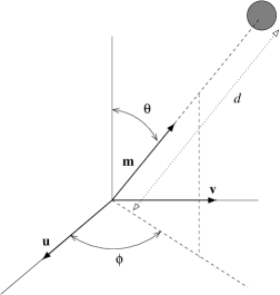
Figure 3: Relative position of the sphere and interferometer.

Figure 4: The behavior of $j_{2}(2\pi fd)$ against the frequency $f$ (Hz) for $d=270$ km, which is approximately the distance between the location of VIRGO and Frascati (resonant spheres).

Figure 4 shows the frequency dependence of this overlap reduction function for a particular choice of the distance $d$ corresponding to the distance between the VIRGO site and Frascati. The most striking aspect, compared to the overlap reduction functions of interferometer-interferometer correlations, is that the correlation vanishes if the distance between the detectors, $d$, goes to zero. This is the opposite of what happens for two interferometers, where instead the correlation is maximum for coincident detectors, so that the ideal strategy in that case would be to have two interferometers as close as possible, compatibly with the fact that local noises, like the seismic noise and local electromagnetic disturbances should be uncorrelated (it is believed that this implies a minimum distance of at least a few tens of kms). In this case, instead, a sphere coincident with an interferometer makes for a totally ineffective correlation. This is easily understood, because the monopole mode of the sphere has, obviously, a constant angular pattern, while an interferometer has a dependence $\sim\cos 2\phi$ which over the solid angle integrates to zero. Parentetically, this shows that in this case the function $\gamma(f)$ cannot be defined, since it should be defined dividing $\Gamma(f)$ for the value for coincident detectors, which is now zero. However, $\Gamma(f)$ is the quantity that enters the SNR.

Of course, as $d\rightarrow\infty$ the overlap reduction function again vanishes, and therefore there is an optimal, finite value for the product of the distance $d$ and the frequency $f$, determined by the maximum of $j_{2}(2\pi fd)$. Approximately, this maximum is reached when

$$\left(\frac{f}{590{\rm Hz}}\right)\left(\frac{d}{270{\rm km}}\right)\simeq 1\,.$$ (57)

We have taken the reference value 270 km, which corresponds to the distance between the locations of VIRGO (Lat. N 43.63, Lon. E 10.50 deg) and Frascati (Lat. N 41.80, Lon. E 12.67 deg). Since the resonant sphere is a narrow band detector, compared to the interferometer, this means that the optimal correlation is obtained with a sphere that resonate at approximately 590 Hz. We see from fig. (4) that the sensitivity of the overall correlation is very strongly affected by the value of $f$, and a value of $f\sim$ 1 kHz, while keeping the sphere in Frascati, can easily result in the loss of more than one order of magnitude in the SNR defined in eq. (41). Note also that the minimum detectable value of $h_{0}^{2}\Omega_{\rm gw}$ is quadratic with the SNR [18] and therefore an inappropriate value of the resonant frquency can easily result in loosing two or three order of magnitude in $h_{0}^{2}\Omega_{\rm gw}$.

Conversely, if for technological reasons the frequency of the resonant sphere has to be fixed at a different value, eq. (57) can be used to obtain the optimal distance between the two detectors.

4 The interaction of the interferometer with a very light scalar

Till now we have considered only massless scalars; it is interesting, having in mind the extension to situations motivated by string theory, to consider the effect of a small mass term on the response of a detector.

Let us first understand what it means ‘small’ in this context. We still want to treat the scalar as a classical wave that acts coherently on the detector. This implies first of all that $m\ll 1/L$, where $L$ is the characteristic size of the detector. For a sphere of size of order 1 meter, this gives approximately $m<10^{-6}$ eV, while for a km sized interferometer $m<10^{-9}$ eV. In both cases, however, there is a stronger limitation that comes from the fact that, if we want to detect these scalars with a detector that works at a frequency $f_{0}=1$ kHz, or $\omega_{0}=2\pi$ kHz, we must require that the frequency of the massive scalar, $\omega_{m}=\sqrt{k^{2}+m^{2}}$, is of order of $\omega_{0}$. Since of course $\omega_{m}\geq m$, we get

$$m<2\pi\,{\rm kHz}\sim 4\times 10^{-12}\,{\rm eV}\,.$$ (58)

For these ultralight scalars it still make sense to discuss their effect as a coherent gravitational wave

In the opposite limit of large mass, the single quanta of the scalar field will behave as particles rather than waves and will interact incoherently with the detector, just with separate hits and since they only interact gravitationally they will be totally unobservable.

Consider the action describing the Jordan–Brans–Dicke theory (1), with in addition a potential term for the scalar:

$${\cal{S}} = {\cal{S}}_{\rm g}+{\cal{S}}_{\rm m}\,,$$

$${\cal{S}}_{\rm g}[g_{\mu\nu},\varphi] = \frac{1}{16\pi}\int\!{\rm d}^{4}x\sqrt{-g}\left[\varphi R-\frac{\omega_{\rm BD}}{\varphi}\>\nabla^{\mu}\varphi\>\nabla_{\mu}\varphi-V(\varphi)\right]\,,$$

$${\cal{S}}_{\rm m}[\psi_{\rm m},g_{\mu\nu}] = \int\!{\rm d}^{4}x\sqrt{-g}\>{\cal{L}}_{\rm m}\left[\psi_{\rm m},g_{\mu\nu}\right]\;.$$ (59)

In analogy with the massless case, to obtain the field equations we vary the action ${\cal{S}}$ with respect to the metric $g^{\mu\nu}$ and to the scalar $\varphi$; then, we linearize the equations near the background $(\eta_{\mu\nu},\varphi_{0})$, where $\varphi_{0}$ is a minimum of $V$. The equations of motion in vacuum (where the matter energy-momentum tensor $T_{\mu\nu}$ is zero) are

$${\cal{R}}_{\mu\nu}-\frac{{}_{1}}{{}^{2}}{\cal{R}}\>\eta_{\mu\nu} = -\partial_{\mu}\partial_{\nu}\Phi+\eta_{\mu\nu}\Box\Phi$$ (60)

$$\Box\Phi-m^{2}\Phi = 0\;,$$ (61)

where

• ${\cal{R}}_{\mu\nu},{\cal{R}}$ are the linearized (with respect to $h_{\mu\nu}\equiv(g_{\mu\nu}-\eta_{\mu\nu})\>$) Ricci tensor and scalar curvature;

• $\Phi\equiv-(\varphi-\varphi_{0})/\varphi_{0}$ ;

• $\displaystyle{m^{2}\equiv\frac{V^{\prime\prime}(\varphi_{0})\>\varphi_{0}}{(3+2\omega_{\rm BD})}}$ .

Again in analogy to the massless case, the linearized Riemann tensor ${\cal{R}}_{\mu\nu\rho\sigma}$ and the equations (60) and (61) are invariant under gauge-transformations

$$\left\{\begin{array}[]{rclcl}h_{\mu\nu}(x)&\to&h_{\mu\nu}^{\prime}(x)&=&h_{\mu\nu}(x)-\partial_{(\mu}\epsilon_{\nu)}\\ \varphi(x)&\to&\varphi^{\prime}(x)&=&\varphi(x)\;;\end{array}\right.$$ (62)

we then define

$$\theta_{\mu\nu}\equiv h_{\mu\nu}-\eta_{\mu\nu}\left(\frac{{}_{1}}{{}^{2}}h-\Phi\right)$$ (63)

and choose the Lorentz gauge (in analogy to electromagnetism)

$$\partial_{\mu}\theta^{\mu\nu}=0\;,$$ (64)

by means of a transformation such that $\Box\epsilon_{\nu}=\partial^{\mu}\theta_{\mu\nu}$. In such a gauge the field-equations become wave-equations:

$$\Box\theta_{\mu\nu} = 0$$ (65)

$$\Box\Phi = m^{2}\Phi\;,$$ (66)

whose solutions are plane waves (and superpositions of them):

$$\theta_{\mu\nu}(x) = A_{\mu\nu}(\vec{k})e^{ik_{\alpha}x^{\alpha}}+{\rm c.c.}$$ (67)

$$\Phi(x) = b(\vec{k})e^{iq_{\alpha}x^{\alpha}}+{\rm c.c.}\;,$$ (68)

where:

$$\begin{array}[]{rclcl}k^{\alpha}&\equiv&(\omega_{0};\vec{k})&&\omega_{0}=k\equiv|\vec{k}|\\ q^{\alpha}&\equiv&(\omega_{m};\vec{k})&&\omega_{m}=\sqrt{k^{2}+m^{2}}\;;\end{array}$$ (69)

as one sees from (69), the dispersion law for the modes of $\Phi$ is that of a massive field, and the group-velocity of a wave-packet of $\Phi$ centered in $\vec{k}$ is

$$\vec{v}=\frac{\partial\omega_{m}}{\partial\vec{k}}=\frac{\vec{k}}{\omega_{m}}\;,$$ (70)

exactly the velocity of a massive particle with momentum $\vec{k}$.

As in the massless case, we have a residual gauge-freedom: we remain in the gauge (64) by transformations with $\Box\epsilon_{\nu}=0$. Notice that the Lorentz gauge is a transversality condition on the field $\theta_{\mu\nu}$

$$\partial_{\mu}\theta^{\mu\nu}=0\;\;\Rightarrow\;\;k_{\mu}A^{\mu\nu}=0\;$$ (71)

but it says nothing about the transversality of the perturbation $h_{\mu\nu}=\theta_{\mu\nu}-\eta_{\mu\nu}\left(\displaystyle{\frac{{}_{1}}{{}^{2}}}\theta-\Phi\right)$. And, in fact, it is easy to show that, due to the field equation (66), it is impossible to choose a gauge analogous to (2). In fact, as in the massless case discussed in app. A, to choose such a gauge, we should operate a transformation with:

$$\left\{\begin{array}[]{rcl}\Box\epsilon^{\mu}&=&0\\ \partial_{\mu}\epsilon^{\mu}&=&-\displaystyle{\frac{{}_{1}}{{}^{2}}}\theta+\Phi\;,\end{array}\right.$$ (72)

but now this is not compatible with the wave equations (65), (66). Analogously, we cannot impose any linear relationship between $\theta_{\mu\nu}$ and $\Phi$: so, for example, we cannot choose a gauge in which $h_{\mu 0}=0$, which in the massless case instead permits to integrate immediately the geodesic equation.

Instead, we can choose a gauge in which a gravitational wave propagating in the $+z$ direction takes the form:

$$h_{\mu\nu}(t,z)=A^{(+)}(t-z)\>e^{(+)}_{\mu\nu}+A^{(\times)}(t-z)\>e^{(\times)}_{\mu\nu}+\Phi(t,z)\>\eta_{\mu\nu}\;,$$ (73)

where $e^{(+)}_{\mu\nu}$ and $e^{(\times)}_{\mu\nu}$ are the polarization tensors (3). This is similar to the gauge choice discussed in app. B, but now, because of the non-linear dispersion law, $\Phi$ depends separately on $t$ and $z$, instead of depending only on their difference $t-z$. This makes the discussion of the physical effect of the wave different from the massless case.

To study the effect of the scalar wave on test-masses, we now make use of the proper reference frame of one of these masses (as the beam-splitter of an interferometer, for example): the analysis thus can be performed in newtonian terms (see [20, sect. 13.6]), in the sense that the spatial coordinates $x^{j}$ represent proper distances for the observer ‘sitting’ on the beam-splitter, the time variable $t$ represents his proper time, and the effect of the gravitational wave on test-masses is described by the equation of motion:

$$\frac{{\rm d}^{2}x^{j}}{{\rm d}t^{2}}=-{R^{j}}_{0k0}\>x^{k}\;,$$ (74)

where the quantities ${R^{j}}_{0k0}$ are the so-called electric components of the Riemann tensor. The problem is thus reduced to calculate ${R^{j}}_{0k0}$ in the proper reference frame of this observer: this is connected by an infinitesimal coordinate transformation to the reference frame where eq. (73) holds, and since the linearized Riemann tensor ${\cal{R}}_{\mu\nu\rho\sigma}$ is invariant under infinitesimal gauge transformations, we can compute it from the metric eq. (73). Restricting to a purely scalar GW, a straightforward computation gives

$${{\cal{R}}^{i}}_{0j0}=\frac{{}_{1}}{{}^{2}}\left(\begin{array}[]{ccc}-\partial^{2}_{t}&0&0\\ 0&-\partial^{2}_{t}&0\\ 0&0&m^{2}\end{array}\right)_{ij}\Phi(t,z)=-\frac{{}_{1}}{{}^{2}}T_{ij}\>\partial^{2}_{t}\>\Phi\>+\>\frac{{}_{1}}{{}^{2}}L_{ij}\>m^{2}\Phi\;,$$ (75)

where $T_{ij}\equiv(\delta_{ij}-\hat{n}_{i}\hat{n}_{j})$ is the transverse projector with respect to the direction of propagation ${\bf\hat{n}}$, and $L_{ij}\equiv\hat{n}_{i}\hat{n}_{j}$ the longitudinal projector. The equation of motion (74) thus becomes:

$$\frac{{\rm d}^{2}}{{\rm d}t^{2}}x_{i}=\left(\frac{{}_{1}}{{}^{2}}\partial^{2}_{t}\Phi\right)\cdot T_{ij}x_{j}+\left(-\frac{{}_{1}}{{}^{2}}m^{2}\Phi\right)\cdot L_{ij}x_{j}\;,$$ (76)

from which one immediately sees what is the effect of the dilaton mass: it generates a longitudinal force (in addition to the transverse one) proportional to $m^{2}$. In the limit $m\to 0$ one recovers the treatment of the massless case, confirming again, also from the point of view of the proper reference frame, the results of sect. 2.

To better understand the contribution of $m$, it is convenient to restrict to a wave packet $\Phi(t,z)$ centered at a frequency $\omega_{m}=\sqrt{k^{2}+m^{2}}$; in this case

$$\frac{{\rm d}^{2}}{{\rm d}t^{2}}x_{i}=\left(-\frac{{}_{1}}{{}^{2}}\omega_{m}^{2}\Phi\right)\cdot\left(T_{ij}+\frac{m^{2}}{\omega_{m}^{2}}\>L_{ij}\right)x_{j}\;.$$ (77)

From this equation the physical effect of the mass can be read quite clearly. In particular

• for ultra-relativistic momenta ($\omega_{m}\simeq k\gg m$) the longitudinal components of the force becomes negligible with respect to the transverse one;

• in the non-relativistic limit $\omega_{m}\to m$ and the stress induced by the wave becomes isotropic, as $L_{ij}+T_{ij}=\delta_{ij}$.

Now one can compute the pattern function of a detector for these massive scalar waves. In a generic gauge the response of the detector is obtained contracting the detector tensor $D_{ij}$ with the tensor ${R^{i}}_{0j0}$, which in the massive case is proportional to $\omega_{m}^{2}T_{ij}+m^{2}L_{ij}$. Note that the pattern function of an interferometer for detection of such massive scalar waves is identical to the one computed in the massless case: in fact, the contraction of $\omega_{m}^{2}T_{ij}+m^{2}L_{ij}$ with $D_{ij}$ is the sum of a term containing $D_{ij}T_{ij}$ and a term containing $D_{ij}L_{ij}$; both these terms are proportional to $D_{ij}\>\hat{n}_{i}\hat{n}_{j}$, since $D_{ij}$ is traceless, for an interferometer, and, so the only dependence on the mass $m$ is in the overall factor of the signal and is independent of ${\bf\hat{n}}$. In particular, for $\omega_{m}\to m$ the signal goes to zero. The pattern function is instead mass-dependent in the case of a detector with a non-traceless response tensor, as for the monopole mode of the sphere, or for the common mode of an interferometer, for which $D_{ij}=\hat{u}_{i}\hat{u}_{j}+\hat{v}_{i}\hat{v}_{j}$.

5 The string dilaton and moduli fields

It is clearly important to understand whether these results, that have been obtained in the context of Brans-Dicke theory, can be applied to the physically more interesting case of the dilaton and the other scalar fields predicted by string theory.

While the dilaton-graviton sector of the low energy sector of string theory is the same as a Brans-Dicke theory, the situation is quite different for the interaction of the dilaton with matter. Since in the string case $\omega_{\rm BD}=-1$, the dilaton is coupled with a strength of the same order as the graviton, and produces unacceptable deviations from general relativity, unless a non-zero dilaton mass is generated see e.g. [1]. The radius of the non-universal force that it mediates must be smaller than about 1 cm, or $m>2\times 10^{-5}$ eV. Therefore the analysis of the previous section, which was valid for $m<4\times 10^{-12}$ eV, does not apply to a massive dilaton. Indeed, it is also in general not easy to reconcile such light scalar particles with cosmology, see e.g. [21, 22], although there are mechanisms that solve the cosmological problems created by light scalars, typically introducing a second short stage of inflation that dilutes the dilaton overproduced by oscillations around their quadratic potential.

Actually, there is the possibility to circumvent this bound on the mass, with a mechanism that has been proposed by Damour and Polyakov [2]. Assuming some form of universality in the string loop corrections, it is possible to stabilize a massless dilaton during the cosmological evolution, at a value where it is essentially decoupled from the matter sector. In this case, however, the dilaton becomes decoupled also from the detector, since the dimensionless coupling of the dilaton to matter ($\alpha$ in the notation of [2]) is smaller than $10^{-7}$ (see also [23]). Such a dilaton would then be unobservable at VIRGO, although it could still produce a number of small deviations from General Relativity which might in principle be observable improving by several orders of magnitude the experimental tests of the equivalence principle [24].

So, in both cases, the analysis done for Brans-Dicke theory does not appear to be relevant for string theory. However, it is clear that our present understanding of the string dilaton and moduli is incomplete and presents a number of unsettled issues, including the non-perturbative mechanism for mass generation, or the stabilization at the minimum of the potential [25], and a definite conclusion is probably premature.

Acknowledgments We thank Danilo Babusci, Stefano Braccini, Maura Brunetti, Ramy Brustein, Francesco Fucito and Thibault Damour for useful discussions.

Appendix A Gravitational waves in the Jordan–Brans–Dicke theory

The Jordan–Brans–Dicke theory is described in the Jordan–Fierz frame by the action

$${\cal{S}} = {\cal{S}}_{\rm g}\left[g_{\mu\nu},\varphi\right]+{\cal{S}}_{\rm m}\left[\psi_{\rm m},g_{\mu\nu}\right]$$ (78)

$${\cal{S}}_{\rm g} \equiv \frac{1}{16\pi}\int\!{\rm d}^{4}x\sqrt{-g}\left[\varphi R-\frac{\omega_{\rm BD}}{\varphi}\nabla^{\mu}\varphi\nabla_{\mu}\varphi\right]$$ (79)

$${\cal{S}}_{\rm m} \equiv \int\!{\rm d}^{4}x\sqrt{-g}\>{\cal{L}}_{\rm m}\left[\psi_{\rm m},g_{\mu\nu}\right]\;;$$ (80)

where:

• $g_{\mu\nu}$ is the metric tensor, with which one constructs all the covariant quantities, such as the scalar curvature $R$, covariant derivatives $\nabla$, etc.;

• $\varphi$ is a scalar field;

• $\omega_{\rm BD}$ is a parameter;

• $\psi_{\rm m}$ are the matter fields, such as fermions, gauge fields, etc.;

• ${\cal{L}}_{\rm m}$ is their lagrangian.

To obtain the field equation one as to vary the action ${\cal{S}}$ with respect to $g^{\mu\nu}$ and to $\varphi$; this leads to

$$R_{\mu\nu}-\frac{{}_{1}}{{}^{2}}R\>g_{\mu\nu}=\frac{8\pi}{\varphi}\>T_{\mu\nu}\!\!\! + \!\!\!\frac{\omega_{\rm BD}}{\varphi^{2}}\left[\partial_{\mu}\varphi\>\partial_{\nu}\varphi-\frac{{}_{1}}{{}^{2}}g_{\mu\nu}g^{\alpha\beta}\>\partial_{\alpha}\varphi\>\partial_{\beta}\varphi\right]+$$ (81)

$$+\frac{1}{\varphi}\left[\nabla_{\mu}\partial_{\nu}\varphi-g_{\mu\nu}g^{\alpha\beta}\>\nabla_{\alpha}\partial_{\beta}\varphi\right]$$

$$R-\frac{\omega_{\rm BD}}{\varphi^{2}}\>g^{\mu\nu}\>\partial_{\mu}\varphi\>\partial_{\nu}\varphi\!\!\! + \!\!\!2\frac{\omega_{\rm BD}}{\varphi}\>g^{\mu\nu}\>\nabla_{\mu}\partial_{\nu}\varphi=0\;,$$ (82)

where

$$T_{\mu\nu}\equiv-\frac{2}{\sqrt{-g}}\frac{\delta{\cal{S}}_{\rm m}}{\delta g^{\mu\nu}}$$ (83)

is the matter-fields energy-momentum tensor.

Eq. (81), multiplied by $g^{\mu\nu}$, gives

$$-R=\frac{8\pi}{\varphi}\>T-\frac{\omega_{\rm BD}}{\varphi^{2}}\>\partial_{\mu}\varphi\>\partial^{\mu}\varphi-\frac{3}{\varphi}\>\nabla_{\mu}\partial^{\mu}\varphi$$ (84)

that, substituted in eq. (82), leads to:

$$\frac{(3+2\omega_{\rm BD})}{\varphi}\>\nabla_{\mu}\partial^{\mu}\varphi=\frac{8\pi}{\varphi}\>T\;.$$ (85)

Eqs. (81) and (85) are our basic field equations. We now study small perturbations around a background configuration: we choose as background the Minkowski metric and $\varphi(x)=\varphi_{0}=\displaystyle{\frac{4+2\omega_{\rm BD}}{(3+2\omega_{\rm BD})G}}\>$, in order to have the correct post-Newtonian limit and to obtain General Relativity when $\omega_{\rm BD}\to\infty\>$, as showed in [26]; we consider

$$\left\{\begin{array}[]{rcl}g_{\mu\nu}(x)&=&\eta_{\mu\nu}+h_{\mu\nu}(x)\\ \varphi(x)&=&\varphi_{0}+\delta\varphi(x)\;,\end{array}\right.$$ (86)

with $|h_{\mu\nu}|\ll 1$ and $|\delta\varphi|\ll\varphi_{0}$. We call ${\cal{R}}_{\mu\nu\rho\sigma}$, ${\cal{R}}_{\mu\nu}$ and ${\cal{R}}$ the linearization to first order in $h_{\mu\nu}$ of the corresponding quantities $R_{\mu\nu\rho\sigma}$, $R_{\mu\nu}$ and $R$; one has [20]

$${\cal{R}}_{\mu\nu\rho\sigma}=\frac{{}_{1}}{{}^{2}}\left\{\partial_{\mu}\partial_{\beta}h_{\alpha\nu}+\partial_{\nu}\partial_{\alpha}h_{\mu\beta}-\partial_{\alpha}\partial_{\beta}h_{\mu\nu}-\partial_{\mu}\partial_{\nu}h_{\alpha\beta}\right\}\;.$$ (87)

The linearization of the field-equations (81) and (85) in vacuum ($T_{\mu\nu}=0$) gives

$${\cal{R}}_{\mu\nu}-\frac{{}_{1}}{{}^{2}}\eta_{\mu\nu}{\cal{R}} = -\partial_{\mu}\partial_{\nu}\Phi+\eta_{\mu\nu}\Box\Phi$$ (88)

$$\Box\Phi = 0\;,$$ (89)

with $\Phi(x)\equiv-\delta\varphi(x)/\varphi_{0}$. In analogy to General Relativity, we can define a transformation acting on our fields that leave unchanged the linearized Riemann tensor ${{\cal{R}}^{\mu}}_{\nu\rho\sigma}$ (and consequently equations (88) and (89)): such an infinitesimal gauge transformation with parameter $\epsilon^{\mu}$ is

$$\left\{\begin{array}[]{rclcl}h_{\mu\nu}(x)&\to&h_{\mu\nu}^{\prime}(x)&\equiv&h_{\mu\nu}(x)-\partial_{(\mu}\epsilon_{\nu)}\\ \Phi(x)&\to&\Phi^{\prime}(x)&\equiv&\Phi(x)\;.\end{array}\right.$$ (90)

It is straightforward to verify, by direct substitution in (87), that ${{\cal{R}}^{\mu}}_{\nu\rho\sigma}$ is gauge-invariant. We want to use this gauge freedom to obtain a wave-equation. We thus define

$$\theta_{\mu\nu} \equiv h_{\mu\nu}-\frac{{}_{1}}{{}^{2}}\eta_{\mu\nu}h+\eta_{\mu\nu}\Phi$$ (91)

$$\theta \equiv \eta^{\mu\nu}\theta_{\mu\nu}=-h+4\Phi\;,$$ (92)

with $h\equiv\eta^{\mu\nu}h_{\mu\nu}$; the transformation that expresses $h_{\mu\nu}$ in terms of $\theta_{\mu\nu}$ has the same form

$$h_{\mu\nu} = \theta_{\mu\nu}-\frac{{}_{1}}{{}^{2}}\eta_{\mu\nu}\theta+\eta_{\mu\nu}\Phi$$ (93)

$$h = -\theta+4\Phi\;.$$ (94)

Substituting (93) into (88) one obtains the field equation for $\theta_{\mu\nu}$

$$\Box\theta_{\mu\nu}-\partial_{\mu}\left(\partial^{\alpha}\theta_{\alpha\nu}\right)-\partial_{\nu}\left(\partial^{\alpha}\theta_{\alpha\mu}\right)+\eta_{\mu\nu}\partial^{\beta}\left(\partial^{\alpha}\theta_{\alpha\beta}\right)=0\;.$$ (95)

Inserting eq. (90) into eq. (91) one finds immediately that under gauge-transformations

$$\left\{\begin{array}[]{rcrcl}\theta_{\mu\nu}(x)&\to&\theta_{\mu\nu}^{\prime}(x)&=&\theta_{\mu\nu}(x)-\partial_{(\mu}\epsilon_{\nu)}+\eta_{\mu\nu}\partial^{\alpha}\epsilon_{\alpha}\\ \theta(x)&\to&\theta^{\prime}(x)&=&\theta(x)+2\partial^{\alpha}\epsilon_{\alpha}\\ \Phi(x)&\to&\Phi^{\prime}(x)&=&\Phi(x)\;;\end{array}\right.$$ (96)

By choosing $\epsilon^{\mu}$ such that $\Box\epsilon_{\nu}=\partial^{\mu}\theta_{\mu\nu}$, one has

$$\partial^{\mu}\theta_{\mu\nu}^{\prime}=0\;,$$ (97)

and, so, a wave equation for $\theta_{\mu\nu}^{\prime}$ (see eq. (95))

$$\Box\theta_{\mu\nu}^{\prime}=0\,.$$ (98)

In this gauge (we will call it Lorentz gauge, in analogy to electromagnetism) the solutions are plane waves and their superpositions (we omit the $(\>\>)^{\prime}$)

$$\theta_{\mu\nu}(x) = A_{\mu\nu}(\vec{k})\>e^{i\>k^{\alpha}x_{\alpha}}\>+\>{\rm c.c.}$$ (99)

$$\Phi(x) = b(\vec{k})\>e^{i\>k^{\alpha}x_{\alpha}}\>+\>{\rm c.c.}\;,$$ (100)

with the following conditions (deriving from the field-equations and from (97))

$$k^{\alpha}k_{\alpha} = 0$$ (101)

$$k^{\mu}A_{\mu\nu} = 0\;;$$ (102)

the latter is a transversality condition for $A_{\mu\nu}$.

Once we have chosen the Lorentz gauge, we can still operate transformations with $\Box\epsilon^{\mu}=0$; we thus take $\epsilon^{\mu}$ such that

$$\left\{\begin{array}[]{rcl}\Box\epsilon^{\mu}&=&0\\ \partial_{\mu}\epsilon^{\mu}&=&\displaystyle{-\frac{{}_{1}}{{}^{2}}\theta+\Phi}\end{array}\right.$$ (103)

(it is possible bacause in vacuum in Lorentz gauge $\Box\theta=\Box\Phi=0$);
one has (see (96) and (93))

$$\theta=2\Phi\;\Rightarrow\;h_{\mu\nu}=\theta_{\mu\nu}\;;$$ (104)

that means that $h_{\mu\nu}$ too is a plane transverse wave.

Again, we have not yet completely fixed the gauge: we satisfy our conditions

$$\left\{\begin{array}[]{ccc}\partial^{\mu}\theta_{\mu\nu}&=&0\\ \theta&=&2\Phi\end{array}\right.$$ (105)

also by operating gauge transformations with

$$\left\{\begin{array}[]{rcl}\Box\epsilon^{\mu}&=&0\\ \partial_{\mu}\epsilon^{\mu}&=&0\;.\end{array}\right.$$ (106)

Consider the case in which the wave is propagating in $+z$ direction: then

$$k^{\mu}=(k,0,0,k)$$ (107)

$$k^{\mu}A_{\mu\nu}=0 \>\Rightarrow\> A_{0\nu}=-A_{3\nu}$$ (110)

$$A_{\nu 0}=-A_{\nu 3}$$

$$A_{00}=-A_{30}=+A_{33}\;.$$

Let us make a degrees-of-freedom counting for $A_{\mu\nu}$:

• we started with 10 ($=$ independent components of a symmetric tensor);

• transversality leads to 7: it “kills” only 3 (instead of 4) because of symmetry of $A_{\mu\nu}$;

• the condition $\theta=2\Phi$ leads to 6: we choose $A_{00}$, $A_{11}$, $A_{22}$, $A_{21}$, $A_{31}$, and $A_{32}$ as independent components;

• further gauge freedom permits us to put to zero 3 of the 6 components (three rather than four, because of condition $\partial_{\mu}\epsilon^{\mu}=0$).

Thus taking

$$\left\{\begin{array}[]{rcl}\epsilon_{\mu}(x)&=&\tilde{\epsilon}_{\mu}(\vec{k})\>e^{i\>k^{\alpha}x_{\alpha}}\>+\>{\rm c.c.}\\ k^{\mu}\tilde{\epsilon}_{\mu}&=&0\end{array}\right.$$ (111)

the action of the gauge-transformation on $A_{\mu\nu}$ is (see (96) and (99))

$$A_{\mu\nu}\to A_{\mu\nu}^{\prime}=A_{\mu\nu}-ik_{(\mu}\tilde{\epsilon}_{\nu)}\;;$$ (112)

or, for the 6 components we are interested in,

$$\begin{array}[]{rcl}A_{00}&\to&A_{00}+2\>ik\tilde{\epsilon}_{0}\\ A_{11}&\to&A_{11}\\ A_{22}&\to&A_{22}\\ A_{21}&\to&A_{21}\\ A_{31}&\to&A_{31}-ik\tilde{\epsilon}_{1}\\ A_{32}&\to&A_{32}-ik\tilde{\epsilon}_{2}\;.\end{array}$$ (113)

Notice that $A_{11}$, $A_{22}$ and $A_{21}=A_{12}$ are invariant: we thus choose $\tilde{\epsilon}_{0}$, $\tilde{\epsilon}_{1}$, $\tilde{\epsilon}_{2}$ in order to “kill” the others. We have now completely fixed the gauge.

Does $h_{\mu\nu}$ depend on the field $\Phi$? Eq. (104) tells us $h=h_{11}+h_{22}=2\Phi$.
Summarizing, we can say that, in this gauge, the metric perturbation $h_{\mu\nu}$ produced by a gravitational wave propagating in the $+z$ direction takes the form

$$h_{\mu\nu}(t-z)=A^{(+)}(t-z)\>e^{(+)}_{\mu\nu}+A^{(\times)}(t-z)\>e^{(\times)}_{\mu\nu}+\Phi(t-z)\>e^{\rm(s)}_{\mu\nu}\;,$$ (114)

where $e_{\mu\nu}^{+,\times,\,{\rm s}}$ are given in eqs. (3) and (4).

Appendix B Equivalence of the two gauges

In this appendix we show that it is possible to choose a gauge (which we denote writing a tilde over quantities evaluated in this gauge) in which the metric perturbation $\tilde{h}_{\mu\nu}$ has the form (114), with $\tilde{A}^{(+)}=A^{(+)},\tilde{A}^{(\times)}=A^{(\times)},\tilde{\Phi}=\Phi,\tilde{e}^{(+)}_{\mu\nu}=e^{(+)}_{\mu\nu},\tilde{e}^{(\times)}_{\mu\nu}=e^{(\times)}_{\mu\nu},$ but

$$\tilde{e}^{\rm(s)}_{\mu\nu}={\rm diag}(-1,+1,+1,+1)=\eta_{\mu\nu}\;.$$ (115)

The quantities without a $\tilde{(\>\>)}$ refer to the gauge used in the previous appendix and in section 2.1. We call “transverse” the former gauge, and “conformal” the latter: we want to find a gauge transformation that passes from the transverse gauge to the conformal one. In order to have a wave equation for $\theta_{\mu\nu}$ one has to keep the Lorentz gauge condition: this condition is mantained by imposing $\Box\epsilon_{\mu}=0$. By choosing

$$\left\{\begin{array}[]{rcl}\partial_{\mu}\epsilon^{\mu}&=&-\displaystyle{\frac{{}_{1}}{{}^{2}}\theta}\\ \Box\epsilon^{\mu}&=&0\end{array}\right.$$ (116)

which is possible because in Lorentz gauge in vacuum $\Box\theta=0$, we obtain a traceless $\theta_{\mu\nu}^{\prime}$ and so (see eq. (93))

$$h_{\mu\nu}^{\prime}=\theta_{\mu\nu}^{\prime}+\Phi\>\eta_{\mu\nu}\;.$$ (117)

In analogy with appendix A, acting with a transformations with

$$\left\{\begin{array}[]{rcl}\partial_{\mu}\epsilon^{\mu}&=&0\\ \Box\epsilon^{\mu}&=&0\end{array}\right.$$ (118)

we can now eliminate the appropriate components of $\theta_{\mu\nu}^{\prime}$ (see equations (113)), in order to obtain exactly $\tilde{h}_{\mu\nu}$. It is then easy to prove that $\tilde{A}^{(+)}=A^{(+)}$ and $\tilde{A}^{(\times)}=A^{(\times)}$, by examining the action of gauge transformations on those amplitudes.

The two gauges are thus equivalent: and in fact it is easy to exibit the coordinate transformation that relates them (the coordinates with a $(\>\>)^{\prime}$ denote the transverse gauge and we now limit to the case of a purely scalar wave)

$$\left\{\begin{array}[]{rcl}x^{\prime}&=&x\\ y^{\prime}&=&y\\ z^{\prime}&=&z-\displaystyle{\frac{{}_{1}}{{}^{2}}I(t-z)}\\ t^{\prime}&=&t+\displaystyle{\frac{{}_{1}}{{}^{2}}I(t-z)}\;,\end{array}\right.$$ (119)

where

$$I(t-z)\equiv\int^{t-z}_{-\infty}\!\Phi(u){\rm d}u\;.$$ (120)

In fact

$$\left\{\begin{array}[]{rcl}{\rm d}x^{\prime}&=&{\rm d}x\\ {\rm d}y^{\prime}&=&{\rm d}y\\ {\rm d}z^{\prime}&=&\left(1+\displaystyle{\frac{{}_{1}}{{}^{2}}}\Phi\right){\rm d}z-\displaystyle{\frac{{}_{1}}{{}^{2}}}\Phi\>{\rm d}t\\ {\rm d}t^{\prime}&=&\left(1+\displaystyle{\frac{{}_{1}}{{}^{2}}}\Phi\right){\rm d}t-\displaystyle{\frac{{}_{1}}{{}^{2}}}\Phi\>{\rm d}z\;,\end{array}\right.$$ (121)

and

$${\rm d}s^{2}=(1+\Phi)(-{\rm d}t^{2}+{\rm d}x^{2}+{\rm d}y^{2}+{\rm d}z^{2})=\eta_{\mu\nu}\>{\rm d}{x^{\prime}}^{\mu}{\rm d}{x^{\prime}}^{\nu}+\Phi\>({\rm d}{x^{\prime}}^{2}+{\rm d}{y^{\prime}}^{2})\,.$$ (122)

As we have seen in section 2.1, the physical meaning of the primed coordinates is that they are comoving with free-falling test-masses, initially at rest, and $t^{\prime}$ is proper time. We can check this assertion in the conformal gauge, by making use of the solution of the geodesic equations of motion found in [15], see eq. (22). By substituting eq. (22) into the transformations (119) one finds

$$\left\{\begin{array}[]{rcl}x^{\prime}(t)&=&x_{0}\\ y^{\prime}(t)&=&y_{0}\\ z^{\prime}(t)&=&z_{0}\\ t^{\prime}(t)&=&t+z(t)-z_{0}=\tau(t)+{\rm const}\;,\end{array}\right.$$ (123)

that proves that, in the primed coordinates, bodies initially at rest remain at rest.

Appendix C Relationship between $S_{h}(f)$ and $\Omega_{\varphi}(f)$

When dealing with stochastic backgrounds of ordinary GWs one defines $S_{h}(f)$ as follows [18]. One expands the metric perturbation in plane waves

$$h_{ij}(t,\vec{x})=\sum_{A=+,\times}\int_{-\infty}^{+\infty}\!{\rm d}f\int\!{\rm d}\Omega_{\bf\hat{n}}\>h_{A}(f,{\bf\hat{n}})\>e^{2\pi i\>f(t-\vec{x}\cdot{\bf\hat{n}})}\>e^{A}_{ij}({\bf\hat{n}})\;,$$ (124)

where the ensemble average of the Fourier modes is

$$\langle\>h_{A}^{*}(f,{\bf\hat{n}})\>h_{A^{\prime}}(f^{\prime},{\bf\hat{n}}^{\prime})\>\rangle=\delta(f-f^{\prime})\>\frac{1}{4\pi}\>\delta^{2}({\bf\hat{n}},{\bf\hat{n}}^{\prime})\>\delta_{AA^{\prime}}\>\frac{1}{2}\>S_{h}(f)\;,$$ (125)

and $\delta^{2}({\bf\hat{n}},{\bf\hat{n}}^{\prime})\equiv\delta(\phi-\phi^{\prime})\>\delta(\cos\theta-\cos\theta^{\prime})\>$. By inserting eq. (124) in the expression $\rho_{\rm gw}=1/(32\pi G)\>\langle\>\dot{h}_{ij}\dot{h}_{ij}\>\rangle$ for the energy density of the background, one obtains

$$\rho_{\rm gw}=\frac{4}{32\pi G}\int_{f=0}^{f=+\infty}\!{\rm d}(\log f)\>f\>(2\pi f)^{2}\>S_{h}(f)\;,$$ (126)

so that

$$S_{h}(f)=\frac{3H_{0}^{2}}{4\pi^{2}f^{3}}\>\Omega_{\varphi}(f)\;.$$ (127)

In the case of scalar waves, we write

$$h^{\rm(s)}_{ij}(t,\vec{x})=\int_{-\infty}^{+\infty}\!{\rm d}f\int\!{\rm d}\Omega_{\bf\hat{n}}\>h_{\rm(s)}(f,{\bf\hat{n}})\>e^{2\pi i\>f(t-\vec{x}\cdot{\bf\hat{n}})}\>e^{\rm(s)}_{ij}({\bf\hat{n}})\;,$$ (128)

and

$$\langle\>h_{\rm(s)}^{*}(f,{\bf\hat{n}})\>h_{\rm(s)}(f^{\prime},{\bf\hat{n}}^{\prime})\>\rangle=\delta(f-f^{\prime})\>\frac{1}{4\pi}\>\delta^{2}({\bf\hat{n}},{\bf\hat{n}}^{\prime})\>\frac{1}{2}\>S_{h}(f)\;.$$ (129)

We want to relate this new function $S_{h}(f)$ to the energy density $\rho_{\varphi}$ of the field $\varphi$. It is convenient to rewrite the field-equation of the Jordan–Brans–Dicke theory in the Einstein frame, that it is related to the Jordan–Fierz one by the conformal transformation

$$g_{\mu\nu}^{\rm E}\equiv\left(\frac{\varphi}{\varphi_{0}}\right)g_{\mu\nu}\;.$$ (130)

In this frame, the field-equation for the metric has the standard General Relativity form

$$R_{\mu\nu}^{\rm E}-\frac{{}_{1}}{{}^{2}}g_{\mu\nu}^{\rm E}\>R^{\rm E}=\frac{8\pi}{\varphi_{0}}\>T_{\mu\nu}^{\rm E}+\frac{3+2\omega_{\rm BD}}{2\varphi^{2}}\left[\partial_{\mu}\varphi\>\partial_{\nu}\varphi-\frac{{}_{1}}{{}^{2}}g_{\mu\nu}^{\rm E}\>g^{\alpha\beta}_{\rm E}\>\partial_{\alpha}\varphi\>\partial_{\beta}\varphi\right]\;,$$ (131)

and the energy-momentum conservation law becomes

$$\nabla_{\rm E}^{\nu}\left[T^{\rm E}_{\mu\nu}+\frac{(3+2\omega_{\rm BD})\varphi_{0}}{16\pi\>\varphi^{2}}\left(\partial_{\mu}\varphi\>\partial_{\nu}\varphi-\frac{{}_{1}}{{}^{2}}g_{\mu\nu}^{\rm E}\>g^{\alpha\beta}_{\rm E}\>\partial_{\alpha}\varphi\>\partial_{\beta}\varphi\right)\right] \equiv$$

$$\equiv\nabla_{\rm E}^{\nu}\left[T^{\rm E}_{\mu\nu}+T^{(\varphi)}_{\mu\nu}\right]=0\;,$$ (132)

so we define $T^{(\varphi)}_{\mu\nu}$ as the energy-momentum tensor of the field $\varphi$. To first order in $h_{\mu\nu}^{\rm E}\equiv(g_{\mu\nu}^{\rm E}-\eta_{\mu\nu})$ and $\Phi\equiv\displaystyle{-\left(\frac{\varphi-\varphi_{0}}{\varphi_{0}}\right)}$ we have

$$T^{(\varphi)}_{\mu\nu}=\frac{(3+2\omega_{\rm BD})\varphi_{0}}{16\pi}\left(\partial_{\mu}\Phi\>\partial_{\nu}\Phi-\frac{{}_{1}}{{}^{2}}\eta_{\mu\nu}\>\partial^{\alpha}\Phi\>\partial_{\alpha}\Phi\right)\;;$$ (133)

the energy density is

$$\rho_{\varphi}\equiv T^{(\varphi)}_{00}=\frac{(3+2\omega_{\rm BD})\varphi_{0}}{32\pi}\left[\dot{\Phi}^{2}+\left(\vec{\nabla}\Phi\right)^{2}\right]\;,$$ (134)

that, by using field equation $\Box\Phi=0$ and averaging over several wave-lengths, reduces to

$$\rho_{\varphi}=\frac{(4+2\omega_{\rm BD})}{32\pi G}\langle\>2\dot{\Phi}^{2}\>\rangle\;,$$ (135)

where we used $\varphi_{0}=(4+2\omega_{\rm BD})/G(3+2\omega_{\rm BD})$, as discussed in app. A. As $h_{ij}^{\rm(s)}=\Phi\>e_{ij}^{\rm(s)}$, using eqs. (128) and (129) we have

$$\rho_{\varphi} = \frac{(4+2\omega_{\rm BD})}{32\pi G}\langle\>\dot{h}^{\rm(s)}_{ij}\dot{h}^{\rm(s)}_{ij}\>\rangle=$$ (136)

$$= \frac{2(4+2\omega_{\rm BD})}{32\pi G}\int_{f=0}^{f=+\infty}\!{\rm d}(\log f)\>f\>(2\pi f)^{2}\>S_{h}(f)\;,$$ (137)

so that

$$S_{h}(f)=\frac{3H_{0}^{2}}{4\pi^{2}f^{3}}\>\frac{1}{2+\omega_{\rm BD}}\>\Omega_{\varphi}(f)\;.$$ (138)

References

- [1] T.R. Taylor and G. Veneziano, Phys. Lett. B213 (1988) 450.
- [2] T. Damour and A.M. Polyakov, Nucl. Phys. B423 (1994) 532.
- [3] M. Bianchi, E. Coccia, C. Colacino, V. Fafone and F. Fucito, Class. Quant. Grav. 13 (1996) 2865.
- [4] P. Astone et al., in Second Amaldi Conference on Gravitational Waves, E. Coccia, G. Pizzella and G. Veneziano eds., (World Scientific, Singapore, 1998), pg. 551.
- [5] M. Bianchi, M. Brunetti, E. Coccia, F. Fucito, and J.A. Lobo, Phys. Rev. D57 (1998) 4525.
- [6] M. Brunetti, E. Coccia, V. Fafone and F. Fucito, Phys. Rev. D59 (1999) 044027.
- [7] M. Brunetti, Tesi di Laurea, Roma 1996 (unpublished).
- [8] S. Merkowitz and W. Johnson, Phys. Rev. D51 (1995) 2546, Phys. Rev. D53 (1996) 5377, Phys. Rev. D56 (1997) 7513.
- [9] E. Coccia, V. Fafone, G. Frossati, J. Lobo and J. Ortega, Phys. Rev. D57 (1998) 2051.
- [10] D.L. Lee, Phys. Rev. D10 (1974) 2374.
- [11] A. Giazotto, Phys. Rept. 182 (1989) 365.
- [12] P.R. Saulson, Fundamentals of Interferometric Gravitational Wave Detectors, World Scientific, Singapore, 1994.
- [13] R. Forward, Gen. Relativ. Gravit. 2 (1971) 149.
- [14] E. Flanagan, Phys. Rev. D48 (1993) 2389.
- [15] M. Shibata, K. Nakao and T. Nakamura, Phys. Rev. D50 (1994) 7304.
- [16] A. Nicolis, Tesi di Laurea, Pisa 1999 (unpublished).
- [17] B. Allen, The Stochastic Gravity-Wave Background: Sources and Detection, in Les Houches School on Astrophysical Sources of Gravitational Waves, eds. J.A. Marck and J.P. Lasota, (Cambridge University Press, 1996); gr-qc/9604033.
- [18] M. Maggiore, Gravitational Wave Experiment and Early Universe Cosmology, gr-qc/9909001, Phys. Rept., in press.
- [19] N. Christensen, Phys. Rev. D46 (1992) 5250.
- [20] C. Misner, K. Thorne and J. Wheeler, Gravitation, Freeman, N.Y., 1973.
- [21] B. de Carlos, J.A. Casas, F. Quevedo and E. Roulet, Phys. Lett. B318 (1993) 447.
- [22] T. Banks, D.B. Kaplan and A.E. Nelson, Phys. Rev. D49 (1994) 779.
- [23] T. Damour and G. Esposito-Farèse, Class. Quant. Grav. 9 (1992) 2093.
- [24] T. Damour, Experimental Tests of Relativistic Gravity, gr-qc/9904057.
- [25] R. Brustein and P. Steinhardt, Phys. Lett. B302 (1993) 196.
- [26] C.M. Will, Theory and Experiment in Gravitational Physics, Cambridge University Press, Cambridge, 1993.