The cosmological model with an analytic exit from inflation.

Abstract

A cosmological model of homogeneous and isotropic spatially flat Universe with gravitating self-interacting scalar field is considered. The exact solution, admitting an analytical exit from inflationary stage into a radiation era and a matter dominated epoch, is obtained by virtue of “fine turning of the potential” method. We found that an inflationary stage is supported by decay of higgs bosons in the framework of the solution obtained. Freidmann’s regim is associated with adiabatical expantion of the Universe, filled by the matter with special equation of state.

Thus we presented the exact solution which solve the problem of transition from an inflationary to a radiation eras or long standing ‘exit’ problem.

PACS-94: 04.20.-q  98.80.-Dr

1 Introduction

In this contribution we investigate general properties of the evolution of a homogeneous isotropic universe on the basis of an analysis of the system of Einstein equations for a self-interacting scalar field. One of the important requirements imposed on early universe theories by present-day observational data is the existence of an inflationary phase in the evolution of the universe with the scale factor increasing at an exponential rate.[1] Thus the morden general consept of universe’s evolution include the evolution from the Planck’s epoch through an inflationary stage which should be ended by exit to radiation era and then to matter dominated epoch to the present-day universe. In a literature we can find a lot of theories which can describe all of mentioned epochs, but separately, that is the the physical content of the model is changed from one regim to enother. Therefore it is important to construct the model of one physical content describing the global evolution of the Universe starting from the preinflationary epoch and ending with later epochs in the evolution of the universe. The model of this kind should have a solution of ‘exit problem’ from inflation stage to radiation and matter dominated stage, mentioned in the original work of A.Guth [2] as a central problem of inflationary scenario. In the present work we present the exact solution, admitting an analytical exit from inflationary stage into a radiation era and a matter dominated epoch. The result is obtained by virtue of “fine turning of the potential” method and by the analysis of some correspondence between exact solutions and approximate ones in slow roll regim. We found that an inflationary stage is supported by decay of higgs bosons in the framework of the solution obtained. Freidmann’s regim is associated with adiabatical expantion of the Universe, filled by the matter with special equation of state.

2 Survey of exact solutions in inflation

The inflationary phase of the (isotropic and homogeneous) universe is customarily understood to mean the period $t_{i}<t<t_{f}$ of its early evolution, beginning at the time $t_{i}$ and ending at the time $t_{f}$, when the scale factor $R(t)$ increased at an accelerated rate, i.e.,

$$\ddot{R}=R(H^{2}+\dot{H})>0$$

(see [13]). In this setting the term subinflation is used when $\dot{H}<0$, standard or exponential inflation when $\dot{H}=0$, and superinflation in the case $\dot{H}>0$.

We take a special look at the case in which the law governing the variation of the scale factor $R(t)$ has one of the forms

$$R(t)=R_{0}t^{m},\quad m>1,R_{0}>0,$$ (1)

$$R(t)=R_{0}e^{H_{0}t},\quad H_{0}>0,$$ (2)

$$R(t)=R_{0}(t_{*}-t)^{n},\quad n<0,\quad t_{*}>t_{i},$$ (3)

which establish the general inflation condition $\ddot{R}>0$. The scale factor (1) corresponds to subinflation and is called power-law inflation. The case of superinflation (3) is unattainable within the scope of self-interacting scalar field theory.

The existence of an inflationary period of expansion of the universe is necessary for solving the horizon (homogeneity), flatness, and relic monopole problems, which have been discussed in detail, for example, in the original work of Guth [2] (see also Linde’s book [1]). The specific mechanism driving inflation in the theory with a self-interacting scalar field (inflaton field) is usually identified with the form of the functional dependence of the effective self-interaction potential of the scalar field on the field itself: $V=V(\phi)$. An important factor here in substantiating the existence of such a mechanism is the slow-roll regime, i.e., a regime in which the variation of the field $\phi$ [and the potential $V(\phi)$] was relatively slow, so that the “kinetic” energy of the scalar field can be disregarded: $\dot{\phi}^{2}\ll V(\phi)$ ([14]).

In the standard model (2) the self-interaction potential is specified as a quadratic function of $\phi$:

$$V(\phi)=\mu^{2}\phi^{2}+b.$$

For this case the field varies linearly with time: $\phi\propto t$, whereas the scale factor increases exponentially: $R(t)\propto e^{Ht}$ ([1] and [15]).

A new approach to the construction of exact solutions in inflationary cosmology (without any reliance on the slow-roll regime) has been developed in [12, 16], and [6]. The method can be broadly summarized as follows. We specify the regime of evolution of the scale factor $R=R(t)$ and determine the evolution of the self-interaction potential $V=V(\phi)$ in such a way as to ensure the specified $R=R(t)$ regime. We then determine the rate of change of the scalar field $\dot{\phi}(t)$. Next, integrating over t, we find the law of evolution of the scalar field $\phi=\phi(t)$, which will also be matched with the regime chosen for the scale factor. In the final analysis we obtain a parametric dependence $V=V(\phi)$, which then represents the self-interaction potential “fine-tuned” to the given exact solution.

In previous work, [12] in particular, the self-interaction potentials have been plotted as a function of the scale factor $R(t)$ corresponding to the inflationary regimes (1) and (2). Also in [12] $V(\phi)$ has been obtained in general parametric form for certain types of large-t asymptotic behavior of $R(t)$ such as to ensure regime (1) or (2).

A somewhat different approach to the construction of exact solutions in cosmological inflation models has been presented by Barrow.[17] The crux of his approach is that the evolution of the scalar field $\phi=\phi(t)$ is specified; the next step is to determine the evolution of the scale factor $R=R(t)$ and the potential, which depends explicitly on the scalar field $\phi$.

We also mention the work of Maartens et al.,[18] who have used a method similar to fine tuning of the potential, but with a special parameter introduced in place of time. This approach might well be practical for the solution of some problems, but it complicates the process of obtaining and analyzing solutions.

Here we follow the general scheme of the potential fine-tuning method and submit two new techniques for constructing classes of exact inflationary solutions for a homogeneous and isotropic universe. One technique entails a variational formulation of the conditions underlying the slow-roll regime, and the second rests on the possibility of specifying the self-interaction potential as a function of time. We investigate the general implications of such an approach and present new exact solutions. We proposed as well the cosmological model based on exact solutions in which the quality solution of the global evolution of the universe is found.

The main attention is consentrated on the solution of the exit problem from inflation, because the trasition from radiation- to matter-dominated epochs have beed well investigated [8, 21].

Let us remember that the exit from inflationary stage should be accompanied by the set of Freidmann’s epoch when the scalar factor has the power law evolution $R(t)\propto t^{s},$ where $~{}s<1$. Besides $s=1/2$ – when radiation-dominated and $s=2/3$ when matter-dominated epochs are realized. Let us mention also that each value of $s$ correponds to certain equation of state in standard theory of Big Bang [8].

For the models of the early univers’s evolution, based on the theory of self-interacting scalar field, the inflationary regim is not specific one because it can be provided by a wide class of the potentials of self-interaction [5, 7]. Nevertheless the condition of transition from inflationary regim to freidmann’s stages is a specific one and can be realized under very special restrictions.

We whould like to mention here again the work [18] where the inflationary model with an analytical exit to radiation stage and dust matter is proposed. As a difference from our approuch, the dependence of the Hubbll’s ‘constant’ $H\equiv{\dot{R}}/{R}$ of $\ln R$ is used in [18]; the e-fold number is chosen as one more dynamical variable as well.

3 Exact solution and self-interaction potential for the slow-roll regime

The Einstein equations for a homogeneous isotropic universe, given an arbitrary form of the self-interaction potential $V(\phi)$ of the scalar field $\phi(t)$, can be represented by two equations in the class of Friedmann metrics [12]:

$$V(t)=\frac{1}{\kappa}\left(\Lambda+\frac{\ddot{R}}{R}+2\frac{\dot{R}^{2}}{R^{2}}+\frac{2\epsilon}{R^{2}}\right),$$ (4)

$$\phi(t)=\pm\sqrt{\frac{2}{\kappa}}\int\sqrt{-\frac{d^{2}{\rm ln}{R}}{dt^{2}}+\frac{2\epsilon}{R^{2}}}dt+\phi_{0},$$ (5)

where $\kappa$ is the gravitational constant, $\Lambda$ is the cosmological constant, and $\phi_{0}$ is a constant of integration. This system of equations provides the basis of the potential fine-tuning method. As mentioned in the Introduction, once the evolution of the scale factor has been specified, this method can be used to find the appropriate form of the self-interaction potential to achieve the given regime of evolution of the universe.

The method has been used previously [12, 4] to analyze inflationary regimes and to demonstrate the existence of a large number of self-interaction potentials admitting such an evolution. The enormous diversity of potentials leading to inflation compels us to look for an additional principle that might be used to isolate the potential that actually occurred in the early stages of evolution of the universe. Considering the special importance of the existence of the slow-roll regime for an inflationary scenario, we look into a nonstandard formulation of the slow-roll regime. We define the slow-roll regime with the aid of the variational principle of minimum variation of the scalar field $\phi$ with variation of the scale factor $R(t)$ and, as a consequence, minimum variation of the values of the potential $V(\phi)$. On the basis of Eq.  (5) this condition can be specified by the variational equation

$$\delta\phi=\int\limits_{t_{1}}^{t_{2}}\delta\sqrt{-\frac{d^{2}{\rm ln}{R}}{dt^{2}}+\frac{2\epsilon}{R^{2}}}dt=0,$$ (6)

where $t_{i}\leq t_{1}<t_{2}\leq t_{f}$. This condition literally means that the evolution of the scale factor must be such that the difference in the values of the field $\phi$ in any finite time interval $[t_{1},\,t_{2}]$ will be the smallest among all other possible evolutions. The variation of the values of the potential $V(\phi)$ is also the smallest in this case.

If we introduce the notation

$$F(t)=\left(-\frac{d^{2}{\rm ln}{R}}{dt^{2}}+\frac{2\epsilon}{R^{2}}\right)^{-1/2},$$

the Euler-Lagrange equations corresponding to the variational problem [15] assume the form of a pair of equations for $F(t)$ and $R(t)$:

$$-\frac{d^{2}{\rm ln}{R}}{dt^{2}}+\frac{2\epsilon}{R^{2}}=\frac{1}{F^{2}},$$ (7)

$$\frac{d^{2}F}{dt^{2}}+\frac{2\epsilon}{R^{2}}F=0.$$ (8)

Exact solutions of this system are the simplest to find for the case $\epsilon=0$, which corresponds to a Friedmann flat-space universe. In this case we deduce the following from Eqs.  7) and (8):

$$-\frac{d^{2}{\rm ln}{R}}{dt^{2}}=\frac{1}{F^{2}},\quad\frac{d^{2}F}{dt^{2}}=0.$$

The solution of these equations is given by the functions

$$R(t)=k_{0}(a_{0}t+b_{0})^{{1}/{a_{0}^{2}}}e^{c_{0}t},\quad F(t)=a_{0}t+b_{0},$$ (9)

where $a_{0}$, $b_{0}$, $c_{0}$, and $k_{0}$ are arbitrary constants. Substituting the solution (9) into Eqs.  (4) and [14], we obtain the following results for the field and the potential:

$$\phi(t)=\sqrt{\frac{2}{\kappa}}\,\frac{1}{a_{0}}{\rm ln}(a_{0}t+b_{0})+\phi_{0},$$ (10)

$$V(\phi,c_{0})=\frac{1}{\kappa}\left[\Lambda+3c_{0}^{2}+\left(\frac{3}{a_{0}^{2}}-1\right)e^{-2\alpha(\phi-\phi_{0})}+\frac{6c_{0}}{a_{0}}e^{-\alpha(\phi-\phi_{0})}\right],$$ (11)

where $\alpha=a_{0}\sqrt{\kappa/2}\,$. It is interesting to note that the solution (9)–(11) generalizes a solution obtained previously[19] using the method of generation of new solutions by means of invariant transformations of $\phi$, R, and V, which do not alter the equations of the standard inflation model. As should be expected, the given solution describes an inflationary regime of the exponential or power-law type or a combination thereof.

The solution (10), (11) can be associated with the equation of state of matter on the basis of the analogy between self-interacting scalar field theory and an ideal fluid. This analogy, in particular, is expressed in the fact that by comparing the energy-momentum tensors of these two models one can formally calculate the pressure p and the energy density $\rho$ of an ideal fluid in terms of the parameters of the scalar field model according to the rule

$$T_{4}^{4}=\rho=\frac{1}{2}\dot{\phi}^{2}+V(\phi),$$ (12)

$$-T_{1}^{1}=-T_{2}^{2}=-T_{3}^{3}=p=\frac{1}{2}\dot{\phi}^{2}-V(\phi).$$ (13)

Substituting the expressions for the self-interaction potential $V(\phi)$ from Eq.  (11) and the field $\phi$ from Eq.  (10), we obtain the relations

$$\rho=\frac{1}{\kappa}\left[\Lambda+3c_{0}^{2}+\frac{3}{a_{0}^{2}}e^{-2\alpha(\phi-\phi_{0})}+\frac{6c_{0}}{a_{0}}e^{-\alpha(\phi-\phi_{0})}\right],$$

$$p=-\frac{1}{\kappa}\left[\Lambda+3c_{0}^{2}+(\frac{3}{a_{0}^{2}}-2)e^{-2\alpha(\phi-\phi_{0})}+\frac{6c_{0}}{a_{0}}e^{-\alpha(\phi-\phi_{0})}\right].$$

Eliminating the field $\phi$ from these equations, we obtain an effective equation of state of matter in the form

$$p=-\rho+\frac{2a_{0}^{2}}{\kappa}\left(-c_{0}+\sqrt{\frac{1}{3}(\kappa\rho-\Lambda)}\,\right)^{2}.$$ (14)

When the class of solutions (9)–(11) is extrapolated to small and large times, i.e., beyond the limits of the inflationary phase $t_{i}\leq t_{1}<t_{2}\leq t_{f}$, the following characteristics are readily established. The given solution always begins from a singular state, i.e., for any model parameters ($\Lambda,\,a_{0},\,c_{0},\,b_{0}$) there is a time $t_{0}=-b_{0}/a_{0}$ in the history of the evolution of the scale factor when $R(t_{0})=0$, after which the scale factor increases at an accelerated rate for some time. A natural transition to Friedmann expansion does not take place at larger times, and this is a drawback of the analyzed solutions. The transition to the Friedmann regime requires that $1/a_{0}^{2}=2/3$ and $c_{0}=0$. It is therefore obvious that without the cosmological constant $\Lambda$ in Eq.  (4) its role is assumed by $c_{0}$, and the condition $c_{0}=0$ corresponds to the standard departure from the inflationary regime.[1]

Again we emphasize that the resulting analytical solution (9)–(11) corresponds to an exactly tuned potential in the slow-roll regime in the variational formulation.

It is a well-known fact that the pioneering work on inflation (see the surveys in [1, 14], and [15]) treated a truncated system of Einstein and scalar field equations, with the slow-roll regime defined in such a way as to eliminate the second time derivative of the scalar field $\ddot{\phi}$ from the equations, a device justified by the condition $\dot{\phi}^{2}\ll V(\phi)$. There are no significant constraints on the self-interaction potential in this approach. In our case we have obtained an exact profile of the potential in the explicit form (11). We note once again that a solution analogous to (11) has been obtained previously,[19] but without any mention of the slow-roll regime per se. It is easily verified that the condition $\dot{\phi}^{2}\ll V(\phi)$ is satisfied in a certain time period $t_{i}\leq\Delta t<t_{f}$ for the exact solution (9)–(11).

4 Generation of exact solutions for a given potential V = V(t)

The problem of analyzing the interrelationship between the scenario of evolution of the universe and the form of the self-interaction potential can be treated in time scales greater than the inflationary phase. In this section, with a view toward completeness, we discuss the overall evolution of the universe.

In the standard approach the Einstein equations contain the self-interaction potential of the scalar field in the form of the function $V=V(\phi)$. In our approach $V(\phi)$ is actually replaced by the function $V(t)$, which must be interpreted as an effective potential of material fields. We note that in the given case of a homogeneous and isotropic universe the representation of the self-interaction potential in the form $V=V(t)$ does not conflict with the general variational problem of the derivation of the Einstein equations, where significant use is made of the functional dependence $V(\phi)$, since each function $V(t)$ and $\phi(t)$ corresponds one-to-one with a particular function $V(\phi)$. We call the function $V(t)$ the evolution of the potential energy or the potential history, underscoring the departure of our approach from the standard approach, in which the dependence $V=V(\phi)$ is fixed.

We consider the problem of finding all possible types of evolution of the universe for a fixed potential history $V=V(t)$ describing the time variation of the potential energy of material fields. Stated in the indicated form, the problem has exact solutions, whose construction reduces to the integration of linear equations in the case $\epsilon=0$. We write Eq.  (4) as an equation for the function $Z(t)=Z^{3}$:

$$-\ddot{Z}+3(\kappa V(t)-\Lambda)Z-6\epsilon Z^{1/3}=0.$$ (15)

In the case of a flat-space universe ($\epsilon=0$) this equation acquires the form of an ordinary linear differential equation

$$-\ddot{Z}+3(\kappa V(t)-\Lambda)Z=0,$$ (16)

which has the same form as the Schrödinger equation for the motion of a quantum particle in one-dimensional space with a particle potential energy $U(t)=3\kappa V(t)$ and self-energy $E=3\Lambda$. Now the function $Z(t)$ assumes the role of the particle wave function. We wish to examine this case in more detail.

We assume that one of the solutions of this equation for a fixed dependence $V=V(t)$ has been found. We denote it by $Z_{1}(t)$, whereupon a second linearly independent solution of this equation $Z_{2}(t)$ for a fixed function $U(t)$ is easily found, because any two linearly independent solutions of Eq.  (16) are related by the equation,

$$Z_{1}\dot{Z}_{2}-Z_{2}\dot{Z}_{1}=W_{0},$$ (17)

where $W_{0}$ is a constant. From this result we obtain

$$Z_{2}=Z_{1}\left(Q_{0}+W_{0}\int\frac{dt}{Z_{1}^{2}}\right),$$ (18)

where $Q_{0}$ is a constant of integration. All solutions of Eq.  (16) corresponding to a specified fixed potential $U(t)$ can be found by varying the constants $Q_{0}$ and $W_{0}$.

For example, the solution (9) for $R(t)$ in the problem with a minimally varying field leads to the solutions

$$R_{2}(t) = R_{0}(t)\left[Q_{0}+W_{0}\int R^{-6}(t){dt}\right]^{1/3}$$ (19)

$$= k_{0}(a_{0}t+b_{0})^{1/a_{0}^{2}}e^{c_{0}t}\left[Q_{0}+k_{0}^{6}W_{0}\int{dt}{(a_{0}t+b_{0})^{-6/a_{0}^{2}}e^{-6c_{0}t}}\right]^{1/3}.$$

In the case of pure power-law inflation $C_{0}=0$ in the solution (9) with the minimally varying scalar field we obtain a general class of solutions for $V(t)$ fixed in (10):

$$R_{2}^{(p)}(t) = k_{0}(a_{0}t+b_{0})^{1/a_{0}^{2}}\left[Q_{0}+k_{0}^{6}W_{0}\int{dt}{(a_{0}t+b_{0})^{-6/a_{0}^{2}}}\right]^{1/3}=$$ (20)

$$= k_{0}(a_{0}t+b_{0})^{1/a_{0}^{2}}\left[Q_{0}+k_{0}^{6}W_{0}A{(a_{0}t+b_{0})^{-6/a_{0}^{2}+1}}\right]^{1/3},$$

where $A=a_{0}^{2}/(a_{0}^{2}-6)$.

Note that the solutions (19) and (20) are new exact solutions for a parametric dependence $V=V(\phi)$, i.e., $V=V(t)$, $\phi=\phi(t)$, indicated in the solution (10)–(11).

The proposed method based on (17) carries over without too much difficulty to the case $\epsilon\neq 0$. It is necessary here to fix the function

$$Q(t)=3(\kappa V(t)-\Lambda)-6\epsilon Z^{-2/3}$$

as a time function. The potential $V(t)$ then depends on the form of the solution. The case $\epsilon\neq 0$ requires separate investigation.

The linearity of Eq.  (16) for the function $Z(t)$ permits the formulation of a problem in eigenfunctions and eigenvalues, the role of which is taken here by the cosmological constant, provided that the given equation is augmented with homogeneous initial conditions. For example, we can investigate all possible evolutions for a fixed function $V(t)$ such that evolution begins at a certain time $t_{0}$ from the state $R(t)=Z(t)=0$ and returns to the same singular state at another time $t_{1}>t_{0}$. Such scenarios of the evolution of the universe can be set in correspondence with oscillating solutions [21]: The universe originated and disappeared in the time period $(t_{0},\,t_{1})$. The corresponding problem appears as follows:

$$-\ddot{Z}+3(\kappa V(t)-\Lambda)Z=0,$$ (21)

$$Z|_{t=t_{0}}=0,\quad Z|_{t=t_{1}}=0.$$ (22)

This problem has the same form as quantum-mechanical problems for a discrete spectrum. If the initial conditions are set at times $t_{0}=-\infty$ and $t_{1}=+\infty$, and the potential energy is a smooth function of time, the universe can evolve from other than a singular state and again evolve into a nonsingular state in the sense that the energy densities and other physical characteristics of matter (field) are finite. Other types of homogeneous initial conditions are also possible. The fact that only a finite or denumerable set of admissible values of the cosmological constant occurs for each problem of this kind can shed light on the issue of the true value of the cosmological constant and the physical reasons for it.

5 Analysis of the evolution of the universe for various types of potentials

The determination of the special characteristics of the origin and evolution of various inflationary regimes can be pursued on the basis of the representation (16) in the example of a series of models that are simple from the standpoint of the construction of solutions but are interesting from the standpoint of the behavior of the potentials. In the present study we have chosen the following model potentials in this category:

$$3\kappa V(t)=2t^{2},$$ (23)

$$3\kappa V(t)=\frac{m}{t^{2}},\quad m={\rm{\rm const}},$$ (24)

$$3\kappa V(t)=-\frac{2\lambda_{0}}{\cosh^{2}(\lambda_{0}t)}.$$ (25)

We investigate the solutions for the potentials (23), (24), and (25) from the viewpoint of the possible existence of inflationary regimes and their transition to a Friedmann phase of evolution.

(a) It is readily verified that the potential (23) admits oscillating solutions corresponding to the statement of the problem in the form (21), i.e., laws of the evolution of the scale factor such that the universe goes from a singularity in the limit $t\to-\infty$ to a new singularity in the limit $t\to+\infty$. Thus, the solutions of Eq.  (16), subject to null boundary conditions as $t\to\pm\infty$, have the form

$$Z(t)=H_{i}(t)e^{-t^{2}/2},$$

where $H_{i}(t)$ are Hermite polynomials. For example, the simplest solution has the form $Z(t)=d_{0}^{3}\exp\{-t^{2}/2\}$. In this case

$$R(t)=d_{0}\exp\{-t^{2}/6\},\quad\phi(t)=\pm\sqrt{\frac{2}{3\kappa}}\,t+\phi_{0},\quad V(\phi)=(\phi(t)-\phi_{0})^{2}.$$

The value of the cosmological constant ensuring this evolution regime is $\Lambda=1/3$ (in appropriate units of measurement for the given problem). For this particular solution the condition

$$\ddot{R}=(d_{0}/3)\exp\{-t^{2}/6\}\{{t^{2}}/{3}-1\}>0$$

implies the start of inflation at $t>\sqrt{3}\,$ and no exit from the inflationary regime.

Other Hermite polynomials correspond to higher absolute values of $\Lambda=1,\,5/3,\dots\,$. The evolution regimes in this case are such that the universe passes through a singular state several times. It is readily verified that the inflationary phase for these oscillating solutions begins at $t\to-\infty$, where the scale factor has a zero minimum, and ends at a time $t_{0}$ corresponding to an inflection point of the function $R=R(t)$.

(b) Potentials of the type (24) for $m\geq=1/4$ are interesting because in the case $\Lambda=0$ they describe all possible types of power-law evolution of the scale factor, including power-law inflation. In fact, the general solution of Eq.  (21) for arbitrary $m>0$ and $\Lambda=0$ has the form

$$Z(t)=C_{1}t^{\alpha}+C_{2}t^{\beta},$$ (26)

where $\alpha$ and $\beta$ are distinct solutions of the algebraic equation $x^{2}-x-m=0$, i.e.,

$$\alpha=\frac{1}{2}+\sqrt{\frac{1}{4}+m}>0,\quad\beta=\frac{1}{2}-\sqrt{\frac{1}{4}+m}<0.$$

It is evident from this result that in the case $C_{1}>0$, $C_{2}>0$ the solution (26) is positive at $t>0$ and has one minimum at a point $t_{0}>0$; after passage through this minimum, power-law inflation begins at a time $t_{1}>t_{0}$, asymptotically approaching the $t^{\alpha/3}$ regime. The asymptotic power-law inflation regime corresponds to the requirement $\alpha>3$, so that $m>6$. We note that prior to the time $t_{1}$ the field $\phi$ is imaginary, and the evolution regime physically achieved in the self-interacting scalar field model begins precisely at $t_{1}$. To circumvent this problem, it must be required that the conditions $C_{1}>0$ and $C_{2}\leq 0$ hold. In this case evolution begins from a singular state at a time $t_{S}$ and makes an immediate transition to power-law inflation.

Remarkably, the only regime of power-law evolution of the scale factor that does not lead to the potential (24) is Friedmann expansion with the ultimately rigid state of matter $p=\rho$, for which $R(t)\propto t^{1/3}$, so that $Z\propto t$ and $V(t)=-0$ for $\Lambda=0$. The Friedmann expansion regime $R(t)\propto t^{1/3}$ sets in as $t\to\infty$ subject to the condition that as the potential decreases, it tends to zero more rapidly than $1/t^{2}$. An example of this kind of behavior is afforded by one of the possible functional dependences $R=R(t)$, based on evolution of the form

$$Z(t)=z_{0}+\frac{t^{2}}{1+t}.$$

At $t>-1$ the scale factor passes through a minimum value $z_{0}^{1/3}$ at the time $t=0$, after which inflation begins. Inflation ends when the inflection point is reached, and then as $t\to+\infty$, the evolution asymptotically settles into the Friedmann regime $R(t)\propto t^{1/3}$. The self-interaction potential in this case is

$$V(t)=\frac{\Lambda}{\kappa}+\frac{2}{3\kappa(1+t)^{2}}\,\frac{1}{t^{2}+z_{0}t+z_{0}},$$

whence it follows that

$$V(t)\to\frac{2}{3\kappa}\,\frac{1}{t^{4}}\quad{\rm as}\quad t\to\infty.$$

For transition to the Friedmann regime with dustlike matter, i.e., when $p=0$, it is sufficient that $V(t)\to 2/t^{2}$ as $t\to\infty$. For any other equation of state of the type $p=\gamma\rho$, $\gamma={\rm const}$, it is sufficient that $V(t)\to m/t^{2}$, $m\geq-1/4$ as $t\to\infty$. The case $m=-1/4$ corresponds to a radiation-dominated state of matter.

The potential (24) also leads to oscillating solutions for $m<0$, which correspond to $\Lambda<0$. For example, the general solution of Eq.  (16) for the potential (24) in the case $m=-2$, $\Lambda<0$ has the form

$$Z(t)=A\left(k-\frac{1}{t}\right)e^{kt}+B\left(-k-\frac{1}{t}\right)e^{-kt},\quad k=\sqrt{-3\Lambda}.$$ (27)

The set of solutions of Eq.  (27) includes one that satisfies the condition $Z(\pm\infty)=0$. It is the solution corresponding to $\Lambda=0$ and has the form $Z=A/|t|$, $A>0$.

(c) To discern certain characteristics of the limitations imposed on the growth rate by the condition for transition to Friedmann expansion, we give additional consideration to the history of the potential (25). Like the potential (23), it increases as $t\to\infty$, but only to a finite value equal to zero. In this case the solution for $Z(t)$ with $\Lambda<0$ has the form

$$Z(t)=A(\lambda-\lambda_{0}\tanh(\lambda_{0}t))e^{\lambda t}+B(\lambda+\lambda_{0}\tanh(\lambda_{0}t))e^{-\lambda t}.$$

Here $\lambda^{2}=-3\Lambda>0$. For $\lambda=\lambda_{0}$ this potential corresponds to an oscillating evolution of the form

$$Z(t)=\frac{C}{\cosh(\lambda_{0}t)},\quad R(t)=C^{1/3}\cosh^{-1/3}(\lambda_{0}t),$$

where C is an arbitrary constant. This is a unique solution for the given potential at $\lambda=\lambda_{0}$, corresponding to a unique bound state. As in the case of the potential (23), it describes an inflationary regime in the interval $(-\infty,\,t_{0})$, where $t_{0}$ is the inflection point of the function $R(t)$.

In the case $\lambda=\Lambda=0$ the solution is the function

$$R(t)=C\tanh^{1/3}\lambda_{0}t,$$

which describes the progress of evolution from a singular state at the time $t=0$ to its asymptotic transition to the stationary state $R=C={\rm const}$ as $t\to+\infty$.

In the case $\lambda>\lambda_{0}$, $A>0$, $B=0$ we have the solution

$$Z(t)=A(\lambda-\lambda_{0}\tanh(\lambda_{0}t))e^{\lambda t},\quad R(t)=A^{1/3}e^{\lambda t/3}\left(\lambda-\lambda_{0}\tanh(\lambda_{0}t)\right)^{1/3},$$

which describes evolution without singularities and with the onset of the inflationary regime beginning at a time $t_{0}>0$.

The solutions corresponding to $\Lambda>0$ are oscillating solutions with multiple passages through the value $Z=0$. It is evident that asymptotic Friedmann expansion does not occur for this potential.

Comparing the solutions obtained for the three potential types, we arrive at the following conclusions. First, potentials that increase as $t\to\infty$ [potentials (23) and (25)] do not allow any transition to the Friedmann regime if the growth rate of the potential energy exceeds the rate at which the function $mt^{-2}$ with $m=-1/4$ approaches zero. Transition to the Friedmann regime requires that the potential decrease with time according to a power law of the type $mt^{-2}$ with $m>0$ or that it increase by an analogous law with $-1/4<m<0$. Second, all three potential types exhibit the existence of the inflationary regime, corroborating the conclusion that this regime is not selective with regard to the form of the potential. Altogether these considerations indicate that the most preferred models are those of the type (24), which require slight modifications to ensure transition to the required Friedmann regime. For example, one such modification is the introduction of a weak dependence of m in the equation for the potential (24) on the temperature T of matter

$$V(t,T)=\frac{m(T)}{t^{2}}$$ (28)

such that $m(T)>0$ near the minimum of $R(t)$ and that $m(T)\to 2$ in the limit $t\to\infty$. For example, the required dependence $m(T)$ can be one with jumps characterizing phase transitions in early universe matter. The potential (11) falls in this category in the case $c_{0}=0$. Consequently, these potentials (24) satisfy the slow-roll principle in the variational formulation set forth in Sec.  3.

It should also be noted that the simplicity of the potential equation (28) is preserved only when it is written in the form $V=V(t)$. If the form of the function $V=V(\phi,\,T)$ is written on the basis of the solutions obtained for $R(t)$ and $\phi(t)$, this function acquires an intricate form and depends significantly on the constants of integration of Eq.  (16), which, in turn, are determined by the initial conditions for $R(t)$ and $\phi(t)$. This consideration demonstrates the preferability of the representation $V=V(t)$ over $V=V(\phi)$ for analysis of the model dynamics.

6 The exact and approximate solutions of inflationary models

The standard cosmological model of SSF, including an inflationary stage, in the case of spatially-flat homogeneous and isotropic universe is described by the following system of equations [1]

$$H^{2}=\frac{\ae}{3}\left(\frac{1}{2}{\dot{\phi}}^{2}+V(\phi)\right),$$ (29)

$${\ddot{\phi}}+3H{\dot{\phi}}=-\frac{d}{d\phi}V(\phi)$$ (30)

where $\phi$ is a scalar field, $V(\phi)$ is a self-interaction potential of the scalar field,

$$H(t)=\frac{d}{d{t}}{\rm ln}R(t),$$

$R(t)$ is a scalar factor, $\ae$ is a gravitational constant. The usual process of construction of approximate solutions for inflationary regim consist of neglecting of the values $\ddot{\phi}$ and $\dot{\phi}^{2}$ in comparision with $H\dot{\phi}$ and $H^{2}$. This is the basis of the slow roll approximation. As a result of such procedure the equations above reduced to the following simple form

$$H^{2}=\frac{\ae}{3}V_{(}\phi),$$ (31)

$$3H{\dot{\phi}}=-\frac{d}{d\phi}V_{(}\phi),$$ (32)

in which thier integration is a more simple task. For example, follow by the review [11], one can obtain

$$R_{(}\phi)=R_{0}\exp\{-\ae\int\frac{V}{V^{\prime}}d\phi\}$$ (33)

For the potential in the trancased equations (31)-(32) and for thiers solutions (33) the index “ ” will be used.

We prove here that the exact equations (29)-(30) can be presented in the form of approximate ones (31)-(32) with the help of an effective potential of self-interaction introduced in consideration. We have the formal relation

$$\dot{\phi}=U(\phi)$$ (34)

where $U(\phi)$ is a function of $\phi$. The relation (34) is true for any dependence $\phi=\phi(t)$. Let us introduce now an effective potential $W(\phi)$ following by the rule

$$W(\phi)=V(\phi)+\frac{1}{2}U^{2}(\phi).$$ (35)

Function $W(\phi)$ represents the total energy of the feild as the function of its value. Using (35) the equations (29)-(30) can be transfermed to

$$H^{2}=\frac{\ae}{3}W(\phi),$$ (36)

$$3H{\dot{\phi}}=-\frac{d}{d\phi}W(\phi),$$ (37)

As easily seen, with the accuracy of the exchange of $V_{(}\phi)$ on $W(\phi)$ equations (36),(37) are equivalent to trancased equations (31), (32). A scalar factor (33) in the exact model is

$$R(\phi)=R_{0}\exp\{-\ae\int\frac{W}{W^{\prime}}d\phi\}$$ (38)

or

$$R(t)=R_{0}\exp\{-\int\limits_{t_{0}}^{t}\sqrt{\frac{\ae}{3}W(t)}dt\}$$ (39)

The equations of SSF in the form (36)-(37) are the starting point of the model under consideration admitting an exit to the friedmann stage of evolution.

Equations (36),(37) lead to the relation

$$\sqrt{3\ae}UW^{1/2}=-W^{\prime}$$ (40)

which along with (35) describe the relation between functions $W(\phi)$ and $U(\phi)$ in a such a way that just only one of the functions above is arbitrary. By solving this equation respective to $W$ one can obtain

$$W(\phi)=\frac{3\ae}{4}\left(\int U(\phi)d\phi+\sqrt{W_{0}}\right)^{2}\geq 0,$$ (41)

where $\sqrt{W_{0}}$ is a real constant of integration. This means that the total energy and, consequently, the effective potential $W$ is of nonnegative value in the model under consideration.

In future we will use the following terminology for the potentials $V(\phi)$ $W(\phi)$. The potential of SSF $V(\phi)$ presenting in exact equations (29)-(30) will call true or physical potential The effective potential $W(\phi)$ will call effective potential of the total energy (for the sake of brivity – the potential of total energy) with the aim to differ it from the effective potentials widely used in quantum field theories.

7 The model with effective Higgs potential

In order to describe an exit from inflation to Freidmann’s regim under condition $t\to\infty$ we have to formulate an asimptotical conditions of such exit. The sufficient condition following from the observational data is the vanishing of the energy of an inflaton field when $t\to\infty$. Thus we can require the asimptotical condition

$$\frac{1}{2}(\dot{\phi}(t))^{2}+V(\phi)\to 0,~{}~{}{\rm}~{}~{}t\to\infty.$$ (42)

The last can be decomposed for two another conditions

$$\dot{\phi}(t))=U(\phi(t))\to 0,~{}~{}{\rm}~{}~{}t\to\infty,$$ (43)

$$V(\phi(t))\to 0,~{}~{}{\rm}~{}~{}t\to\infty.$$ (44)

One of the simplest models satisfing by the requirement (43) is the model in which

$$\dot{\phi}=U(\phi(t))=u_{0}e^{-\mu t},~{}~{}~{}\mu>0.$$ (45)

For (45) we have

$$\phi(t)=\phi_{\infty}-\frac{u_{0}}{\mu}e^{-\mu t}.$$ (46)

Therefore

$$U(\phi)=\mu(\phi_{\infty}-\phi(t)).$$

Inserting the last relation to (40), one can find

$$W(\phi)=\left(\frac{\lambda}{4}(\phi-\phi_{\infty})^{2}-\sqrt{V_{\infty}}\right)^{2},$$ (47)

$$R(\phi)=R_{0}\exp\left\{-\ae\int\limits_{\phi_{0}}^{\phi}\frac{\lambda(\phi-\phi_{\infty})^{2}-4\sqrt{V_{\infty}}}{4\lambda(\phi-\phi_{\infty})}d\phi\right\}=$$ (48)

$$=R_{0}\exp\left\{\frac{\ae}{8}(\phi_{0}-\phi_{\infty})^{2}\right\}\left(\left|\frac{\phi-\phi_{\infty}}{\phi_{0}-\phi_{\infty}}\right|\right)^{\alpha}\exp\{-\frac{\ae}{8}(\phi-\phi_{\infty})^{2}\}$$

Here

$$\lambda=\mu\sqrt{3\ae},~{}~{}~{}\alpha=\frac{\ae}{\lambda}\sqrt{V_{\infty}}.$$

${V_{\infty}}$ is the value of the potential in the limit $t\to\infty$, and $\phi_{0}$ is the value of the field at the starting moment $t_{0}$. It is easily to check that for the potential (48) the condition (44) is valid for the case if $V_{\infty}=0$.

From the relation (35) one can find the physical potential

$$V(\phi)=\left(\frac{\lambda}{4}(\phi-\phi_{\infty})^{2}-\sqrt{V_{\infty}}\right)^{2}-\frac{1}{2}\mu^{2}(\phi_{\infty}-\phi)^{2}.\\$$ (49)

This is well known potential of $\phi^{4}$-theory with Higgs properties of spontaneous breaking of the symmetry. In accordance with this theory the effective mass of Higgs boson will be equal to

$$M_{h}=\sqrt{\lambda\sqrt{V_{\infty}}+\mu^{2}}.$$

The minimima of the potential $V(\phi)$ are located in the points

$$\phi^{\pm}=\phi_{\infty}\pm 2\sqrt{\lambda\sqrt{V_{\infty}}+\frac{\mu^{2}}{\lambda^{2}}}=\phi_{\infty}\pm 2\sqrt{\mu\sqrt{3\ae V_{\infty}}+\frac{1}{3\ae}}$$

and maximum in the point $\phi_{\infty}$ (see Fig. 1).

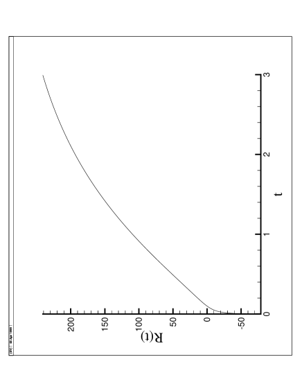
Figure 1: .

In the case $V_{\infty}=0$ we have

$$M_{h}=\mu,~{}~{}~{}\phi^{\pm}=\phi_{\infty}\pm 2\sqrt{\frac{1}{3\ae}}.$$ (50)

The set of formulas (47)-(48), (49) and (46) gives the exact solution for a scale factor of the cosidered model. By inserting in expression for $R(\phi)$ the dependence $\phi=\phi(t)$, one can obtain

$$R(t)=R_{0}\exp\left\{\frac{\ae}{8}(\phi_{0}-\phi_{\infty})^{2}\right\}\left(-\frac{u_{0}}{\mu}\right)^{\alpha}\left(\left|\frac{1}{\phi_{0}-\phi_{\infty}}\right|\right)^{\alpha}e^{-\mu\alpha t}\exp\left\{-\frac{\ae u_{0}^{2}}{8\mu^{2}}e^{-2\mu t}\right\}$$

The condition (44), as it was mention, leads to the requirement $V_{\infty}=\alpha=0$, which give more simple form for scalar factor evolution

$$R(t)=R_{\infty}\exp\left\{-\frac{\ae u_{0}^{2}}{8\mu^{2}}e^{-2\mu t}\right\}.$$ (51)

$$R_{\infty}=R_{0}\exp\left\{\frac{\ae}{8}(\phi_{0}-\phi_{\infty})^{2}\right\}.$$

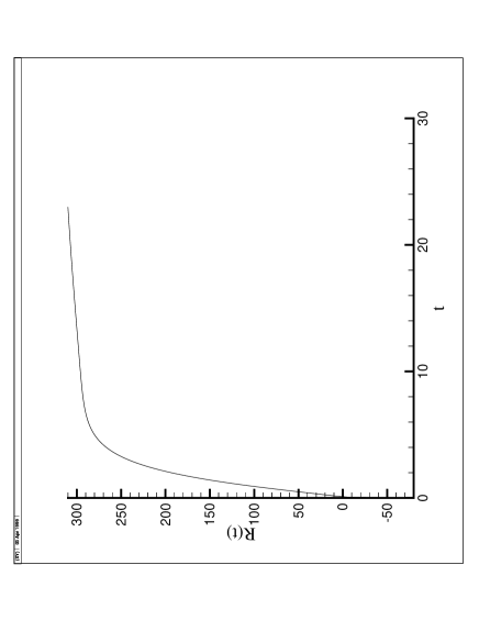
Figure 2: .

This regim of an evolution corresponds to chaotic inflationary model with a massive scalar fiels [1], besides the initial conditions give the following bounds: $U(\phi)\approx M_{P}^{2},~{}~{}u_{0}\approx M_{P}^{2}$, where $M_{P}=\sqrt{\hbar c/G}$ is the Plank’s mass.

It is follow from the relations (50) that the conditions (45) and (46) can be considered as a classical equivalent of decay of Higgs bosons with the mass $M_{h}=\mu$ and with the characteristic time of decay $\tau_{h}\approx 1/\mu$. Thus in the given model it is the decay of Higgs bosons that provide an inflationary temp of expantion. It shoud be mentioned here that this model contains the exit from inflation but to the asimptotically static Universe. Therefore this model can be considered as auxiliary model admitting an important exit property. To obtain a correct asymptotics when $t\to\infty$ the model above shoud be modified with the account of the following fact: the transition to the Freidmann stage is possible if there exists after the moment of Higgs bosons decay a matter in the universe in the condition close to thermodynamical equilibrium with the equation of state $p=\gamma\varepsilon$. In this case an adiabatical expantion of the universe will be of Freidmann type. Using the suggestion above we consider the next auxiliary model.

8 Models with exit to Freidmann’s evolution

In the work [7] (see also the section 3.) have been analysed the evolution’s regim’s corresponding to the condition

$$V(\phi(t))=\frac{m}{3\ae t^{2}}$$ (52)

where $m$ is the constant, which satisfy to the restriction $m\geq-1/4$. In this case the scalar factor’s evolution is determined by

$$R(t)=t^{\beta/3},$$ (53)

where

$$\beta=\frac{1}{2}+\sqrt{\frac{1}{4}+m}>0.$$

The equations of states can be obtained from the formula

$$p=\gamma\varepsilon,~{}~{}~{}\gamma=\frac{\beta-m}{\beta+m}=\frac{1-2m+\sqrt{1+4m}}{1+2m+\sqrt{1+4m}}$$

Generally speaking, the solution (53) can be considered with arbitrary values of $\beta>0$ including a power law inflation under $\beta>3$. But we restrict ourselves by Freidmann’s regims when $0<\beta<3$. The case of power law inflation has been considered in the works [6, 5, 7].

The limiting case $m=-1/4$ corresponds to equation of state with $\gamma=3$, the case $m=0$ – equation of ultrastiff matter with $\gamma=1$, the case $m=2$ – dust matter with $\gamma=0$, and the case $m=3/4$ – pure radiation with $\gamma=1/3$. In general all Freidmann’s regim with $\beta\leq 1$ correspond to condition $-1/4\leq m\leq 6$. The model under consideration corresponds to adiabatical expantion of the universe filled by the matter with an equation of state close to equilibrium one. The special interest is to the radiation era $p=\frac{\epsilon}{3}$ and matter dominated epoch $p\approx 0$ [8].

In the framework of our approach if we have chosen the function $V(t)$ as (52) then

$$U(t)=\frac{\nu}{t}$$ (54)

Under this functional dependence $U$ on $t$ the conditions (43) and (44) are true as well. Following by (34),(35),(36), we obtain the relations

$$\phi(t)=\phi_{1}+\nu{\rm ln}t,~{}~{}U(\phi)=\nu\exp\{-\frac{1}{\nu}(\phi-\phi_{1})\},~{}~{}\phi_{1}={\rm const},$$

$$W(\phi)=\left(\sqrt{V_{1}}+\frac{\sqrt{3\ae}}{2}\nu^{2}\exp\{-\frac{1}{\nu}(\phi-\phi_{1})\}\right)^{2},$$

$$V(\phi)=\left(\sqrt{V_{1}}+\frac{\sqrt{3\ae}}{2}\nu^{2}\exp\{-\frac{1}{\nu}(\phi-\phi_{1})\}\right)^{2}-\frac{1}{2}\nu^{2}\exp\{-\frac{2}{\nu}(\phi-\phi_{1})\}.$$

By inserting in expression for $V(\phi)$ the functions $\phi=\phi(t)$ we obtain

$$V(t)=\left(\sqrt{V_{1}}+\frac{\sqrt{3\ae}}{2}\frac{\nu^{2}}{t}\right)^{2}-\frac{1}{2}\frac{\nu^{2}}{t^{2}}.$$

The dependence $R=R(t)$ is defined from (39) and for the case under consideration it has the form

$$R(t)=R_{0}t^{\ae\nu^{2}/2}\exp\{\sqrt{\frac{\ae}{3}V_{1}}t\}$$ (55)

All possible power law scalar factor’s evolution corresponding to the dependence of the potential energy on time (52), can be obtained in the case $V_{1}=0$. It is the case that one has an axit on Freidmann’s regims (53), besides

$$\beta=\frac{3}{2}\ae\nu^{2}.$$

We have to mention, that in the model under consideration, based on (52) and (54), an inflation is absent, but Freidmann’s regim will appear asimptotically when $t\to\infty$ for any other evolution’s regim differing from (52) and (54) by existing of fast decreasing terms. It is just necessary that the speed of decreasing is over $t^{-2}$ in (52) and $t^{-1}$ in (54), for example, by an exponential rate. This point is the basis for the new model generalizing the results obtained in sections 7 and 8.

9 Inflationary model with the exit to the Freidmann’s expantion.

To construct the model of univers’ evolution with inflationary stage admitting the exit to radiation dominated stage and matter dominated epoch let us consider the linear superposition of the exialary models, which have been considered in the sections 7 8. Namely, let us consider the model corresponding to the relations

$$\dot{\phi}=U(t)=u_{0}e^{-\mu t}+\frac{\nu}{t},$$ (56)

$$\phi(t)=\phi_{c}-\frac{u_{0}}{\mu}e^{-\mu t}+\nu{\rm ln}t.$$ (57)

In this model the conditions (43) are satisfied. Given model has three parameters the meaning of which are clear from preveous analysis of the models (45) and (54). An inflation regim is possible if the period in the history of the evolution exist when

$$u_{0}e^{-\mu t}>>\frac{\nu}{t}$$ (58)

Evidently, we can choose the parameters $\mu,\nu$ and $u_{0}$ in such a way that the condition (58) will be satisfied. Let us show this by direct calculations.

It is difficult to obtain a direct dependence for the function $U=U(\phi)$ using the relations (56) and (57). Nevertheless the presentation in the form of function $U=U(t,\phi)$ is possible. For example,

$$U(\phi,t)=\frac{\nu}{t}+\nu\mu{\rm ln}t-\mu(\phi-\phi_{c})$$

In the present form we can control the deviation the model (56) from the model (54).

Using the relations (40), (56), (57) one can calculate the effective potential $W$

$$W(t)=\left(\sqrt{V_{0}}+\int\limits_{t_{0}}^{t}U^{2}(t)dt\right)^{2}=\left(-\frac{u_{0}^{2}}{2\mu}e^{-2\mu t}-\frac{\nu}{t}+2u_{0}\nu\int\limits_{t_{0}}^{t}\frac{e^{-\mu t}}{t}dt\right)^{2},$$ (59)

$$V(t)=\frac{3\ae}{4}\left(\sqrt{V_{0}}-\frac{u_{0}^{2}}{2\mu}e^{-2\mu t}-\frac{\nu}{t}+2u_{0}\nu\int\limits_{t_{0}}^{t}\frac{e^{-\mu t}}{t}dt\right)^{2}-\left(u_{0}e^{-\mu t}+\frac{\nu}{t}\right)^{2}$$ (60)

We will investigate the potentials $W(\phi)$ and $V(\phi)$ as the functions of time, because it is impossible to find the explisit dependence on $\phi$. For this purpose it is suatable to use the relation (39).

The change of scalar factor $R(t)$ versus the time is shown in the Fig.3 and Fig.4 for the models (56), (57). Fig. 3 corresponds to the period in conventional units before an inflation. Fig. 4 corresponds to the case of general evolution of the universe.

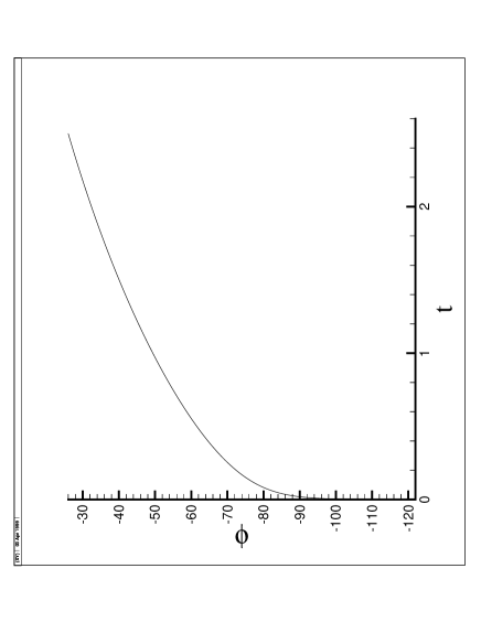
Figure 3: .

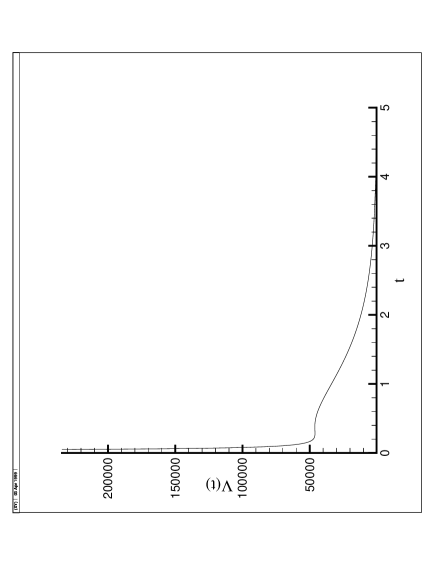
Figure 4: .

The chois of parameters is special for a demonstration of the main effect and equals to $\nu=6,~{}u_{0}=30,~{}\mu=0.3,V_{0}=0,\ae=1$. The change of $\phi=\phi(t)$ and $V=V(t)$ versus time are presented in the figures 5 and 6 using the parameters above.

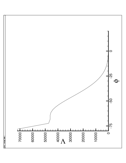
Figure 5: .

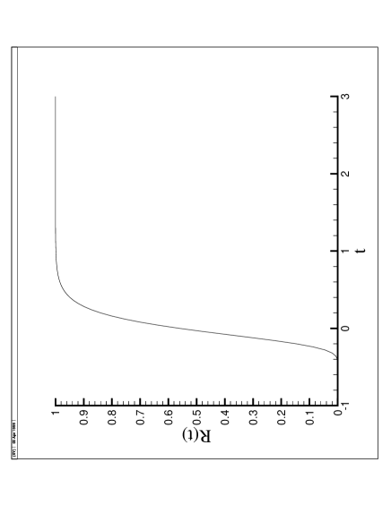
Figure 6: .

The plot of dependence $V=V(\phi)$, calculated by plots of dependence $\phi=\phi(t)$ and $V=V(t)$, is presented in the Fig. 7.

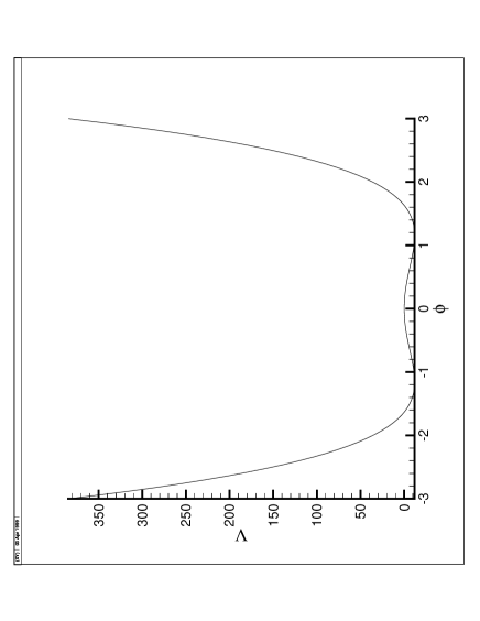
Figure 7: .

Thus during the whole evolution the potential is a positive function and conseiquently the energy dominant condition is true.

10 Conclusion

We have found new classes of exact solutions for a self-consistent system of gravitating scalar fields with self-interaction within the framework of the cosmology of a homogeneous isotropic universe. We have analyzed aspects of the given model that have bearing on the determination of the physical conditions restricting the admissible form of the self-interaction potential and on the determination of the general form of evolution of the scale factor from the standpoint of the existence of an inflationary phase in the evolution of the universe, along with other fundamental characteristics of the potential.

1. We have shown that the definition of the slow-roll regime actively utilized in inflation is amenable to a variational formulation. In this formulation we have obtained an exact solution for the standard model of inflation with a self-interacting scalar field and have given an equation of state of matter corresponding to this solution.

2. We have proposed a method for generating exact solutions with a fixed history of the potential $V=V(t)$. On the basis of the method we have formulated an eigenfunction/eigenvalue problem for a Friedmann flat universe with the role of the eigenvalues taken by the cosmological constant. We have shown that in order to analyze the character of the evolution of the universe, it is simpler to analyze the model dynamics with the potential represented in the form of its history $V=V(t)$ than when it is written as a function of the field $V=V(\phi)$.

3. We have analyzed several characteristic types of potential history and the corresponding evolutions of the scale factor. Our analysis shows that the formal analog of the Einstein equations in the form of the Schrödinger equation (15) or (16) as proposed in this paper can be used to analyze in detail the behavior of various physical factors in self-interacting scalar field models and to discern a potential selection criterion proceeding from physical notions regarding the character of the evolution of the universe in large time scales, including inflation (subinflation) as one of the stages, along with the conditions for transition of the universe into a Friedmann regime. It follows from our analysis that the most realistic model of the history of the potential energy is a model of the form (28).

4.We have constructed the model of the evolution of homogeneous and isotropic universe posessing an inflationary stage with an analitical exit to the radiation dominated epoch and matter dominated era. The model is constructed as a superposition of two auxiliary models, the first of them is responsible for an inflationary stage, while the second – for the Freidmann’s regim including matter dominated epoch.

This work has been carried out with partial financial support from the Russian Foundation for Basic Research (Grant No. 98-02-18040).

References

References

- [1] A. D. Linde, Particle Physics and Inflationary Cosmology (Harwood Acad. Publ., Paris–New York, 1990) [Russ. original, Nauka, Moscow, 1990].
- [2] A. H. Guth, Phys. Rev. D 23, 347 (1981).
- [3] S. V. Chervon, Shchigolev V.K. and V. M. Zhuravlev, Izv. Vyssh. Uchebn. Zaved. Fiz., N 2, 1996, 41.
- [4] S. V. Chervon, Nonlinear Fields in the Theory of Gravitation and Cosmology [in Russian] (Izd. Srednevolzhsk. Nauchn. Tsentra, Ulyanovsk, 1997).
- [5] Chervon S.V., Zhuravlev V.M., Shchigolev V.K. Phys.Let. B 398, 269 (1997).
- [6] S.V.Chervon, Gravitation & Cosmology, v.3, No.2, p.145-150, 1997.
- [7] V. M. Zhuravlev, S. V. Chervon and V. K. Shchigolev, JETP, 114, N 2, 179 (1998).
- [8] Ya.B.Zeldovich, I.D.Novikov, Structure and evolution of the Universe// oscow.:Nauka.-1975.-736 .
- [9] R. Maartens, D. R. Taylor, and N. Roussos, Phys. Rev. D 52, 3358 (1995).
- [10] A.B.Burd, J.D.Barrow, Nucl.Phys., 308, 929 (1988) .
- [11] S.Gottlöber, V.Müller, H.-J.Schmidt and A.A.Starobinsky, Int.J.of Modern Phys. D, 1, No.2, 257 (1992) .
- [12] S. V. Chervon and V. M. Zhuravlev, Izv. Vyssh. Uchebn. Zaved. Fiz., No. 8, 81 (1996).
- [13] P. Coles and F. Lucchin, Cosmology: the Origin and Evolution of Cosmic Structure (Wiley, Chichester, 1995).
- [14] R. H. Brandenberger, in Physics of the Early Universe, Proceedings of the 36th Scottish Universities Summer School in Physics, edited by J. A. Peacock, A. F. Heavens, and A. T. Davies (1989), p. 281.
- [15] V. N. Lukash and I. D. Novikov, in Observational and Physical Cosmology, edited by F. Sunchez, M. Collados, and K. Rebolo (Cambridge Univ. Press, 1990).
- [16] S. V. Chervon and V. M. Zhuravlev, in Abstracts of the Reports at the International School-Seminar “Foundations of Gravitation and Cosmology,” Odessa (RGS, Moscow, 1995), p. 67.
- [17] J. D. Barrow, Phys. Rev. D 49, 3055 (1994).
- [18] R. Maartens, D. R. Taylor, and N. Roussos, Phys. Rev. D 52, 3358 (1995).
- [19] P. Parsons and J. D. Barrow, Class. Quantum Gravity 12, 1715 (1995).
- [20] V. K. Shchigolev, V. M. Zhuravlev, and S. V. Chervon, JETP Lett. 64, 71 (1996).
- [21] S. Weinberg, Gravitation and Cosmology: Principles and Applications of the General Theory of Relativity (Wiley, New York, 1972) [Russ. transl., Mir, Moscow, 1975].