Dynamics of Bianchi IX universe with massive scalar field

Abstract

The dynamics of the Bianchi IX cosmological model with minimally coupled massive real scalar field is studied. The possibility of non-singular transition from contraction to expansion is shown. A set of initial conditions that lead to non-singular solutions is studied numerically.

¹Sternberg Astronomical Institute, Moscow University, Moscow, 119899, Russia

1 Introduction

During last years the dynamics of closed FRW universe with massive minimally coupled real scalar field has become a subject of investigations. Being one of the simplest cosmological models it has a peculiar property. Namely the universe of this type can make a non-singular transition from contraction to expansion (in other worlds a scale factor can posses a local minimum). Such a transition is often referred to as ’bounce’.

It turns out that a universe in principle can make an arbitrary number of bounces. Page [9] was the first who conjectured the presence of a fractal set of infinitely bouncing solutions, later Cornish and Shellard [2] proved that this system is really chaotic. In later works [5]–[7] , [11] the chaotic properties of this and more complicated models were studied.

Numerical investigations have shown that the initial conditions space has a quasi-periodical structure : there are narrow zones which lead to bouncing solutions separated by wide zones which lead to singular solutions. These investigations also have shown that in former zones the solutions exhibits a sensible dependence of initial conditions – a property peculiar to the chaotic dynamical systems. Moreover, starting from one of such zones a solution may pass after bounce through another zone of this type (or through the same one) and suffer a new bounce. After each bounce the situation is similar to the previous one. This lead to the existence of a fractal set of unstable infinitely bouncing solutions. In the dynamical chaos theory such set is called as a strange repellor – a structure which can be found with in many chaotic dynamical systems without dissipation. The presence of this fractal structure of solutions corresponds to the fractal structure of sets of initial conditions leading to bouncing solutions [2].

But the Universe at the earliest stages of its evolution have not necessary had a metric close to FRW one. So for studying the Universe at this time one often invoke more general metrics. The simplest non–FRW metric with positive curvature is the Kantowski–Sachs one. However this case does not include the closed FRW metric, and moreover there are no bouncing solutions in this case (see appendix). More complicated metric is Bianchi IX model. This is the only model that includes closed FRW metric [8]. So in this paper we investigate the Bianchi IX universe with massive scalar field.

The Bianchi IX universe is well known due to its mixmaster approach to singularity [8]. It worth to notice that mixmaster chaos [3, 4] principally differs from the studying one as in the case of mixmaster it is the evolution of anisotropic variables which exhibit chaotic properties while the overall volume of the universe decrease monotonically. In the considered case it is the evolution of the total volume of the universe which exhibit chaotic properties.

2 Equations of motion

Let us consider a Bianchi IX universe with minimally coupled massive scalar field with the action as follows (we use units $c=\hbar=1$, $G=1/{8\pi}$):

$$S=\int\left(-\frac{R}{2}+\frac{1}{2}\varphi_{,i}\varphi^{,i}-\frac{m^{2}}{2}\varphi^{2}\right)\sqrt{-g}\;d^{4}x\;.$$ (1)

The metrics has the following form :

$$ds^{2}=dt^{2}-\eta_{\alpha\beta}(t)\omega^{\alpha}\omega^{\beta}\;,$$ (2)

where

$$\eta_{\alpha\beta}(t)=\left(\begin{array}[]{ccc}a(t)^{2}&0&0\\ 0&b(t)^{2}&0\\ 0&0&c(t)^{2}\end{array}\right)\;,$$ (3)

and $\omega^{\alpha}$ are differential 1–forms invariant under SO(3) transformations.

Assuming $\varphi$ to be a function of time variable only one can write the Einstein’s field equations in following form :

$$\frac{(\dot{a}bc)\dot{}}{abc}+\frac{1}{2a^{2}b^{2}c^{2}}[a^{4}-(b^{2}-c^{2})^{2}]=\frac{m^{2}}{4}\varphi^{2}\;,$$ (4)

$$\frac{(a\dot{b}c)\dot{}}{abc}+\frac{1}{2a^{2}b^{2}c^{2}}[b^{4}-(a^{2}-c^{2})^{2}]=\frac{m^{2}}{4}\varphi^{2}\;,$$ (5)

$$\frac{(ab\dot{c})\dot{}}{abc}+\frac{1}{2a^{2}b^{2}c^{2}}[c^{4}-(a^{2}-b^{2})^{2}]=\frac{m^{2}}{4}\varphi^{2}\;,$$ (6)

$$\ddot{\varphi}+\left(\frac{\dot{a}}{a}+\frac{\dot{b}}{b}+\frac{\dot{c}}{c}\right)\dot{\varphi}+m^{2}\varphi=0$$ (7)

with the first integral of motion :

$$\frac{1}{2}\dot{\varphi}^{2}+\frac{m^{2}}{2}\varphi^{2}=2\left(\frac{\dot{a}}{a}\frac{\dot{b}}{b}+\frac{\dot{a}}{a}\frac{\dot{b}}{b}+\frac{\dot{b}}{b}\frac{\dot{c}}{c}\right)+\frac{1}{a^{2}}+\frac{1}{b^{2}}+\frac{1}{c^{2}}-\frac{a^{4}+b^{4}+c^{4}}{2a^{2}b^{2}c^{2}}\;,$$ (8)

where $\quad\dot{}\equiv\frac{d}{dt}$ .

In our investigation it is more convenient to work with ADM variables $\left\{\Omega(\tau),\beta_{+}(\tau),\beta_{-}(\tau)\right\}$ which are functions of a new time variable $\tau$ : $dt=m^{5}e^{3\Omega}d\tau$ . Relations between ADM variables and the old ones are :

$$\left(\begin{array}[]{c}\Omega\\ \beta_{+}\\ \beta_{-}\end{array}\right)=\left(\begin{array}[]{rrr}\frac{1}{3}&\frac{1}{3}&\frac{1}{3}\\ \frac{1}{6}&\frac{1}{6}&-\frac{1}{3}\\ \frac{\sqrt{3}}{6}&-\frac{\sqrt{3}}{6}&0\end{array}\right)\left(\begin{array}[]{c}\ln a\\ \ln b\\ \ln c\end{array}\right)-\left(\begin{array}[]{c}\ln m\\ 0\\ 0\end{array}\right)\;.$$ (9)

It is easily seen from (9) that variable $\Omega$ describes the volume of the universe while $\beta_{\pm}$ describes it’s anisotropy.

The considered dynamical system admits Hamiltonian formalism. In terms of ADM variables the Hamiltonian has the following form :

$$H=\frac{1}{2}(-p_{\Omega}^{2}+p_{+}^{2}+p_{-}^{2}+\frac{1}{12}p_{\varphi}^{2})+\frac{1}{8}e^{4\Omega}V(\beta_{+},\beta_{-})+\frac{1}{24}\varphi^{2}e^{6\Omega}\;,$$ (10)

where

$$V(\beta_{+},\beta_{-})=\frac{1}{3}(e^{-8\beta_{+}}+2e^{4\beta_{+}}(\cosh 4\sqrt{3}\beta_{-}-1)-4e^{-2\beta_{+}}\cosh 2\sqrt{3}\beta_{-})\;.$$ (11)

The Hamiltonian equations leads to the following :

$$\Omega^{\prime\prime} = \frac{1}{2}e^{4\Omega}V(\beta_{+},\beta_{-})+\frac{1}{4}\varphi^{2}e^{6\Omega},$$ (12)

$$\beta_{+}^{\prime\prime} = \frac{1}{3}e^{4\Omega}\left[e^{-8\beta_{+}}-e^{4\beta_{+}}(\cosh 4\sqrt{3}\beta_{-}-1)-e^{-2\beta_{+}}\cosh 2\sqrt{3}\beta_{-}\right],$$ (13)

$$\beta_{-}^{\prime\prime} = \frac{\sqrt{3}}{3}e^{4\Omega}\left[e^{-2\beta_{+}}\sinh 2\sqrt{3}\beta_{-}-e^{4\beta_{+}}\sinh 4\sqrt{3}\beta_{-}\right],$$ (14)

$$\varphi^{\prime\prime} = -\varphi e^{6\Omega}$$ (15)

and the constraint equation $H=0$ takes the form :

$$-\Omega^{\prime 2}+\beta_{+}^{\prime 2}+\beta_{-}^{\prime 2}+\frac{1}{12}\varphi^{\prime 2}+\frac{1}{4}e^{4\Omega}V(\beta_{+},\beta_{-})+\frac{1}{12}\varphi^{2}e^{6\Omega}=0\;,$$ (16)

where $\quad{}^{\prime}\equiv\frac{d}{d\tau}$ .

To make further investigations we need to generalize the notion of bounce to Bianchi IX case. Being defined as a non-singular transition from contraction to expansion of the universe bounces thus corresponds to local minima of $\Omega$. That is why ADM variables is more preferable choice for our purposes.

Substituting $\Omega^{\prime}=0$ into constraint equation (16) and combining it with the condition $\Omega^{\prime\prime}>0$ it is easily seen that bounces can occur only if :

$$V(\beta_{+},\beta_{-})+\frac{1}{3}\varphi^{2}e^{2\Omega}\leq 0\;,$$ (17)

$$V(\beta_{+},\beta_{-})+\frac{1}{2}\varphi^{2}e^{2\Omega}>0\;.$$ (18)

The above inequalities at least implies $V(\beta_{+},\beta_{-})<0$ which can be satisfied only in a narrow region around the isotropic case $(\beta_{+}=\beta_{-}=0)$ where $V(\beta_{+},\beta_{-})$ suffer it’s minimum. This region is represented on fig. 1 where the levels $V(\beta_{+},\beta_{-})=const$ are shown for the values of $const=-.99$(inner curve), $const=-.90$ , $const=-.75$ , $const=-.50$ and $const=0$(bold lines). The potential has a minimum in point $\beta_{+}=\beta_{-}=0$ (isotropic case) and $V(0,0)=-1$. It also follows from (16) that if a bounce occur the possible values of $\beta_{\pm}^{\prime}$ must satisfy criterion : $\beta_{+}^{\prime 2}+\beta_{-}^{\prime 2}<1$ as $V(\beta_{+},\beta_{-})\geq-1$ for all values of $\beta_{\pm}$ .

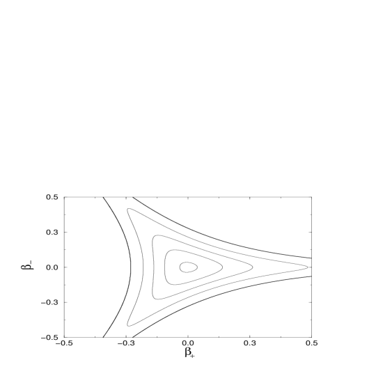
Figure 1: A levels of $V(\beta_{+},\beta_{-})=const$.

Before starting the next section it should be mentioned that Belinsky and Khalatnikov [1] were the first who studied the Bianchi IX model whith scalar field. Thay considered only massless case and found that the presence of the scalar field of this type destroys the Mixmaster oscillatory regime when the universe collapses to singularity. This results holds in massive case as an asymptotic regime.

3 Numerical results

The equations of motion (12)–(15) can be solved numerically. In order to obtain numerical solution one need to fix eight initial conditions. The constraint equation allows to express one of them in terms of the others (in our work we determined $\dot{\varphi}(0)$ in this way). Moreover as the considered system has at least one maximal expansion point (i.e a point where $\Omega$ suffer (local) maximum), one can fix $\Omega^{\prime}(0)=0$ without loss of generality.

For simplicity in our calculations we always fixed $\varphi(0)=0$ . So we studied the dependence of numerical solution from five initial conditions : $\Omega(0)$, $\beta_{+}(0)$, $\beta_{-}(0)$, $\beta_{+}^{\prime}(0)$, $\beta_{-}^{\prime}(0)$ .

The equations of motion have been solved numerically using Bulirsch–Stoer method [10]. As equations (12)–(15) requires evaluations of transcendental functions while equations (4)– (7) requires only arithmetical operations we performed calculations in variables $\left\{a,b,c\right\}$ in order to speed-up them while the initial conditions and results were expressed in terms of $\left\{\Omega,\beta_{+},\beta_{-}\right\}$ . The constraint equation (8) has been used to check the accuracy.

First of all we tested our routines on already known fridmanian case. On fig. 2 we presented a first four closest to singularity simplest symmetric periodical solutions in a projection onto $(\varphi,\Omega)$ plane. Term ’simplest’ means that all of the maximal expansion points for given solution coincide in this plane and symmetric means that these points lies on axis $\varphi=0$. The values of $\Omega$ in the above mentioned points are : $\Omega_{1}=0.160832$ (short dashed line), $\Omega_{2}=0.760135$ (long dashed line), $\Omega_{3}=1.141779$ (dot-dashed line), $\Omega_{4}=1.418301$ (solid line). Near each of these values $\Omega_{i}$ there are narrow intervals which lead to bouncing solutions.

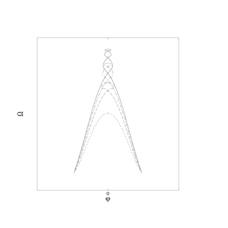
Figure 2: Examples of periodical solutions in Fridmanian case.

As $\Omega^{\prime}(0)=0$ the initial values $\beta_{\pm}(0)$ and $\beta_{\pm}^{\prime}(0)$ have similar restrictions as in the case of bounce with the only exception that (18) is no longer required. Numerical investigations have shown the presence of bouncing solutions only in the case of sufficiently weak anisotropy near the corresponding fridmanian bouncing solutions. These investigations have also shown that for some ranges of initial values of $\Omega$, $\beta_{\pm}$ and $\beta_{\pm}^{\prime}$ solutions exhibits sensible dependence of initial conditions.

To illustrate the structure of the sets of initial conditions which leads to bouncing solutions we calculated a 2d slices through the initial conditions space. For given value of $\Omega(0)$ each slice represents a $500\times 500$ grid in a plane of two of the anisotropy variables while the rest of them equals to zero. For each knot of the grid it has been calculated a numerical solution on a sufficiently large interval of $t\in[0,50]$ . If a maximal value of $\Omega$ on this solution after bounce $\Omega_{max}$ is grater then $\Omega_{4}$ we encoded corresponding dot in a black color. If $\Omega_{4}\geq\Omega_{max}>\Omega_{3}$ we encoded it in a dim gray color. If $\Omega_{3}\geq\Omega_{max}>\Omega_{2}$ we encoded it in a gray color and if $\Omega_{2}\geq\Omega_{max}>\Omega_{1}$ we used a light gray color. We considered only solutions which satisfies criterion $\Omega_{max}\geq\Omega_{1}$ as they are of the most interest. We do not consider the trajectories with the next maximum expantion point lying closer to the singularity than the first bounce interval, becouse in this case the trajectory have only a zigzag, which can not change the fate of the trajectory falling into the singularity.

We calculated such slices for subsequent values of $\Omega$ with sufficiently small steps so that they can be viewed as a ’movie’. Such movies can be found at ”http://www.xray.sai.msu.su/~ustiansk/sciwork/gr-qc/001.html”. Examples of these slices are shown in fig.3–4.

Numerical calculations have shown that there are narrow intervals of initial values $\Omega$ that lead to bouncing solutions separated by wide intervals that lead to singular solutions in full analogy with the fridmanian case. For the closest to singularity interval (an interval which contain $\Omega_{1}$) in a $(\beta_{+},\beta_{-})$ plane one can observe the picture that follows. For the values $\Omega\lesssim 0.1549$ there are no bouncing solutions. With the increase of $\Omega$ bouncing solutions appears in a small region around isotropic case which grow with the growth of $\Omega$ up to the value $\Omega\approx 0.1567$ when a fraction of considered anisotropic bouncing solutions begins to decrease until they vanishes at $\Omega\approx 0.1608$ .

In the case of $(\beta_{+},\beta_{+}^{\prime})$ and $(\beta_{-},\beta_{-}^{\prime})$ slices the general picture slightly differs. With $\Omega$ increasing from the value $\Omega\approx 0.1525$ anisotropic bouncing solutions appears and invoke isotropic case at already mentioned value $\Omega\approx 0.1550$. Thus in considered case the interval of $\Omega$ which allows bouncing solutions becomes slightly wider than in fridmanian one.

For the interval which contain $\Omega_{2}$ the picture is following. For both studied planes $(\beta_{+},\beta_{-})$ and $(\beta_{-},\beta_{-}^{\prime})$ bouncing solutions appears when $\Omega\approx 0.7593$ in a small region around isotropic case. With the growth of $\Omega$ this region grows until $\Omega\approx 0.7603$ . After that the value of $\Omega_{max}$ becomes smaller than $\Omega_{1}$ for initially anysotropy close to zero so such solutions were discarded and thus the region have a ’ring’ shape. For the values $\Omega\approx 0.762$ this regions vanishes. So in considered case the interval of $\Omega$ is wider than in fridmanian one. The similar picture is valid for the interval that contain $\Omega_{3}$.

On several slices one can easily see a narrow ’rings’ (one of them is pointed by two arrows in fig.4) inside the region of initial conditions that lead to bounces. The existence of these ’rings’ is caused by the fact that solutions which correspond to these ’rings’ suffers bounce and the next point of maximal expansion also occurs inside one of the regions that leads to bounce. So such solutions suffer at least two bounces. These ’rings’ forms a fractal structure. The example of such structure is shown in fig.5.

For the splits in $(\beta_{+},\beta_{-})$ it is possible to determine the mesure of bouncing solutions in a simple way if we start from $\varphi(0)=0$. In this case the measure of all possible initial values of $\beta_{\pm}$ , being defined as the area bounded by the bold lines in fig.1 , equals $\sim 0.48$. The maximal fractions of initial values of $\beta_{\pm}$ that lead to acceptable bouncing solutions to all posible initial values for first three subsequent intervales of $\Omega$ are approximately $0.0026$, $0.00041$, $0.00012$.

4 Conclusions

In this paper we studed the Bianki IX cosmological model with the massive scalar field. In particular the influence of initial shear on the possibility of transition from contraction to expansion was investigated. We show that only a very restricted set of initial conditions with shear can led to the bouncing trajectories. Their mesure with respect to all physically admissible initial conditions for the first 3 zones are restricted by $2.6\times 10^{-3}$, $4.1\times 10^{-4}$ and $1.2\times 10^{-4}$ respectively. Corresponding areas of the initial conditions were found numerically also for other cross-sections of the initial conditions space. In all cases, bounces are possible for a ruther narrow zones near corresponding friedmannian trajectory.

On the other hand, the structure of chaos is similar to known in the Friedmann case: there are narrow intervals of initial values $\Omega$ that lead to bouncing solutions separated by wide intervals that lead to singular solutions. The width of the bounce intervals may be enlarged up to $3$ times in comparition with the Friedmann case for the several closest to the singularity intervals, but the qualitative picture is the same one.

Appendix. No chaos in Kantowski–Sachs universe with a massive scalar field

The equations of motion for the Kantowski–Sachs universe filled by a scalar field are

$$\frac{\ddot{b}}{b}-\frac{\dot{a}\dot{b}}{ab}+\frac{\dot{\phi}^{2}}{2}=0,$$ (19)

$$\frac{\ddot{b}}{b}+\frac{\dot{a}\dot{b}}{ab}+\frac{\ddot{a}}{a}+\frac{\dot{\phi}^{2}}{2}=V(\phi),$$ (20)

$$\ddot{\phi}+(\frac{\dot{a}}{a}+2\frac{\dot{b}}{b})\dot{\phi}+V^{\prime}(\phi)=0,$$ (21)

with the constraint

$$2\frac{\dot{a}\dot{b}}{ab}+\frac{\dot{b}^{2}}{b^{2}}+\frac{1}{b^{2}}=\frac{\dot{\phi}^{2}}{2}+V(\phi)$$ (22)

where $a,b$ - the scale factors, $V(\phi)$ - a potential of the scalar field, and the prime indicates the derivative with respect to $\phi$.

It is easy to see from the Eq.(19) that in all the possible turning points with respect to $b$ (i.e. the points in which $\dot{b}=0$), the corresponding acceleration

$$\ddot{b}=-b\dot{\phi}^{2}/2$$ (23)

is always nonpositive, so we can have only the points of maximal expansion for the scale factor $b$.

Combining Eqs.(19 – 20) we receive, on the other side, that the acceleration in the turning points with respect to $a$ is

$$\ddot{a}=aV(\phi),$$ (24)

which is nonnegative for an arbitrary nonnegative scalar field potential $V(\phi)$, and we have only the points of minimal contraction for the scale factor $a$.

As a result, we can claim from Eqs.(23 – 24) that the type of chaos associated with the oscillation of the scale factors is absent in Kantowski–Sachs universe filled by the scalar field with an arbitrary nonnegative potential.

Figure captions

Fig.3: A slice through initial condition space with fixed $\Omega=0.1573$ which represents a $500\times 500$ grid in $(\beta_{+},\beta_{-})$ plane. For each knot of the grid it has been calculated a numerical solution. If a maximal value of $\Omega$ on this solution $\Omega_{max}>\Omega_{4}$ we encoded corresponding dot in a black color. If $\Omega_{4}\geq\Omega_{max}>\Omega_{3}$ we encoded it in a dim gray color. If $\Omega_{3}\geq\Omega_{max}>\Omega_{2}$ we encoded it in a gray color and if $\Omega_{2}\geq\Omega_{max}>\Omega_{1}$ we used a light gray color.

Fig.4: A slice analogous to previous one for the value $\Omega=0.7604$. One of thing rings which represents second order structure is pointed by two arrows. These rings are formed by trajectories which suffer two bounces.

Fig.5: Example of fractal structure in $(\beta_{+},\beta_{-})$ plane with the value of $\Omega=0.7604$. This is a magnified region pointed by two arrows on previous figure. Wide regions represents a second order structure. One can easily see a third order structure as thing lines.

References

- [1] V.A. Belinsky, V.A. Khalatnikov Sov. Phys. JETP 63, 1121 (1972)
- [2] N.J. Cornish, E.P.S. Shellard Phys.Rev.Lett. 81 3571-3574 (1998), gr-qc/9708046
- [3] N.J. Cornish, J.J. Levin Phys.Rev.Lett. 78 998-1001 (1997), gr-qc/ 9605029
- [4] N.J. Cornish, J.J. Levin gr-qc/9709037
- [5] A.Yu. Kamenschik, I.M. Khalatnikov and A.V. Toporensky Int.J.Mod.Phys. D6 673-692 (1997), gr-qc/9801064
- [6] A.Yu. Kamenschik, I.M. Khalatnikov and A.V. Toporensky Int.J.Mod.Phys. D7 129-138 (1998), gr-qc/9801082
- [7] A.Yu. Kamenschik, I.M. Khalatnikov, S.V. Savchenko and A.V. Toporensky Phys.Rev. D59: 123516 (1999), gr-qc/9809048
- [8] C.W. Misner, K.S. Thorne, J.A. Wheeler Gravitation, Freeman and Sons, 1973
- [9] D.N. Page Class. Quant. Grav. 1, 417 (1984)
- [10] W.Press, B.Flannery, S.Teukolsky, W.Vetterling Numerical recipes in C, Cambridge University Press, Cambridge, 1989.
- [11] A.V. Toporensky gr-qc/9812005