Qualitative Analysis of Early Universe Cosmologies

Andrew P. Billyard^1a, Alan A. Coley^1,2b & James E. Lidsey^3c

¹Department of Physics,
Dalhousie University, Halifax, NS, B3H 3J5, Canada

²Department of Mathematics, Statistics and Computing Science,
Dalhousie University, Halifax, NS, B3H 3J5, Canada

³Astronomy Centre and Centre for Theoretical Physics,
University of Sussex, Brighton, BN1 9QJ, U. K.

A qualitative analysis is presented for a class of homogeneous cosmologies derived from the string effective action when a cosmological constant is present in the matter sector of the theory. Such a term has significant effects on the qualitative dynamics. For example, models exist which undergo a series of oscillations between expanding and contracting phases due to the existence of a heteroclinic cycle in the phase space. Particular analytical solutions corresponding to the equilibrium points are also found.

PACS NUMBERS: 98.80.Cq, 04.50.+h, 98.80.Hw

^aElectronic mail: jaf@mscs.dal.ca
^bElectronic mail: aac@mscs.dal.ca
^cElectronic mail: jlidsey@astr.cpes.susx.ac.uk

I Introduction

Very early universe cosmology provides one of the few environments where the predictions of fundamental theories of physics, and in particular string theories, can be investigated. String theory is the most promising candidate for a unified theory of the fundamental interactions. It introduces significant modifications to the standard, hot big bang model based on conventional Einstein gravity and a study of string–inspired cosmologies is therefore important.

String theories predict the existence of a graviton, $g_{\mu\nu}$, a scalar ‘dilaton’ field, $\Phi$, and an antisymmetric two–form potential, $B_{\mu\nu}$, with a field strength $H_{\mu\nu\lambda}\equiv\partial_{[\mu}B_{\nu\lambda]}$ [1, 2]. In four dimensions, the three–form field strength is dual to a one–form, $\nabla_{\mu}\sigma$, such that $H^{\mu\nu\lambda}\equiv e^{\Phi}\epsilon^{\mu\nu\lambda\kappa}\nabla_{\kappa}\sigma$, where $\epsilon^{\mu\nu\lambda\kappa}$ is the covariantly constant four–form [3]. The one–form may be interpreted as the gradient of a scalar ‘axion’ field. The string field equations can then be derived from the effective action [3]

$$S=\int d^{4}x\sqrt{-g}e^{-\Phi}\left[R+\left(\nabla\Phi\right)^{2}-\frac{1}{2}e^{2\Phi}\left(\nabla\sigma\right)^{2}\right]+S_{\rm M},$$ (1)

where $S_{\rm M}$ represents the action for perfect fluid matter sources, $R$ is the Ricci curvature of the spacetime and $g\equiv{\rm det}g_{\mu\nu}$. The dilaton–graviton sector of action (1) may be interpreted as a Brans–Dicke theory, where the coupling parameter between the two fields takes the specific value $\omega=-1$ [4]. The value of the dilaton field determines the effective value of Newton’s ‘constant’, $G_{\rm eff}\propto e^{\Phi}$.

The general solutions to the field equations of action (1) are known analytically when $S_{\rm M}=0$ for both the spatially flat and isotropic Friedmann–Robertson–Walker (FRW) universes and the anisotropic Bianchi type I models [5, 6]. The purpose of the present paper is to qualitatively investigate the consequences of introducing a cosmological constant, $\Lambda_{\rm M}$, into the matter sector of Eq. (1):

$$S=\int d^{4}x\sqrt{-g}\left\{e^{-\Phi}\left[R+\left(\nabla\Phi\right)^{2}-\frac{1}{2}e^{2\Phi}\left(\nabla\sigma\right)^{2}\right]-\Lambda_{\rm M}\right\}.$$ (2)

This term may be interpreted as a perfect fluid matter stress with an equation of state $p=-\rho$. It could be generated by a slowly moving scalar field, with a kinetic energy contribution dominated by a self–interaction potential, $p\approx-V\approx-\rho$. Analytical FRW solutions have not been found for this model when the axion field is trivial and $\Lambda_{\rm M}>0$ [7, 8]. Moreover, the combined effects of the cosmological constant and axion field have not been considered previously.

We determine the general structure of the phase space of solutions for spatially flat FRW and axisymmetric Bianchi type I cosmologies derived from action (2) for arbitrary $\Lambda_{\rm M}$. This complements the work of Refs. [9, 10, 11, 12, 13], where the qualitative effects of introducing a cosmological constant, $\Lambda_{\rm M}\propto e^{-\Phi}$, into the gravitational sector of Eq. (1) were determined.

The paper is organized as follows. In Section 2, the cosmological field equations and solutions for a zero cosmological constant are presented. The qualitative behaviour of the models with positive and negative $\Lambda_{\rm M}$ is determined in Sections 3 and 4, respectively. The phase portraits are interpreted in Section 5 and we conclude with a discussion in Section 6.

II Cosmological Field Equations

The metric for the Bianchi type I model may be written in the form

$$ds^{2}=-dt^{2}+h_{ab}dx^{a}dx^{b},\qquad a,b=1,2,3,$$ (3)

where $h_{ab}(t)$ is a function of cosmic time $t$ only and represents the metric on the surfaces of homogeneity. The axisymmetric model may be parametrized by $h_{ab}=e^{2\alpha(t)}\left(e^{2\beta(t)}\right)_{ab}$, where $e^{3\alpha}$ denotes the effective spatial volume of the universe. The traceless, diagonal matrix $\beta_{ab}\equiv{\rm diag}[\beta,\beta,-2\beta]$ determines the shear of the models and we refer to $\beta$ as the shear parameter [14]. The spatially flat, isotropic FRW model is recovered in the limit where $\beta=0$ and, in this case, $e^{\alpha}$ represents the scale factor of the universe.

Substituting the metric (3) into the action (2) and integrating over the spatial variables implies that

$$S=\int dt~{}~{}e^{3\alpha}\left\{e^{-\Phi}\left[6\dot{\alpha}\dot{\Phi}-6\dot{\alpha}^{2}+6\dot{\beta}^{2}-\dot{\Phi}^{2}+\frac{1}{2}e^{2\Phi}\dot{\sigma}^{2}\right]-\Lambda_{\rm M}\right\},$$ (4)

where the co-moving volume has been normalized to unity without loss of generality and a dot denotes differentiation with respect to $t$. The field equations derived from Eq. (4) are given by

$$\ddot{\alpha} = \dot{\alpha}\dot{\varphi}+\dot{\varphi}^{2}-3\dot{\alpha}^{2}-6\dot{\beta}^{2}-\frac{3}{2}\Lambda_{\rm M}e^{\varphi+3\alpha}$$ (5)

$$\ddot{\varphi} = 3\dot{\alpha}^{2}+6\dot{\beta}^{2}+\frac{1}{2}\Lambda_{\rm M}e^{\varphi+3\alpha}$$ (6)

$$\ddot{\sigma} = -(\dot{\varphi}+6\dot{\alpha})\dot{\sigma}$$ (7)

$$\ddot{\beta} = \dot{\beta}\dot{\varphi},$$ (8)

where

$$\varphi\equiv\Phi-3\alpha$$ (9)

defines the ‘shifted’ dilaton field and the generalized Friedmann constraint takes the form

$$3\dot{\alpha}^{2}-\dot{\varphi}^{2}+6\dot{\beta}^{2}+\frac{1}{2}\dot{\sigma}^{2}e^{2\varphi+6\alpha}+\Lambda_{\rm M}e^{\varphi+3\alpha}=0.$$ (10)

Eqs. (5)–(10) may be simplified by introducing the new time coordinate

$$\frac{d}{d\theta}\equiv e^{-(\varphi+3\alpha)/2}\frac{d}{dt}$$ (11)

and employing the generalized Friedmann constraint equation (10) to eliminate the axion field. The remaining field equations are then given by

$$\alpha^{\prime\prime} = \varphi^{\prime 2}-\frac{9}{2}\alpha^{\prime 2}+\frac{1}{2}\alpha^{\prime}\varphi^{\prime}-6\beta^{\prime 2}-\frac{3}{2}\Lambda_{\rm M}$$ (12)

$$\varphi^{\prime\prime} = 3\alpha^{\prime 2}+6\beta^{\prime 2}-\frac{1}{2}\varphi^{\prime 2}-\frac{3}{2}\alpha^{\prime}\varphi^{\prime}+\frac{1}{2}\Lambda_{\rm M}$$ (13)

$$\beta^{\prime\prime} = \frac{1}{2}\beta^{\prime}\left(\varphi^{\prime}-3\alpha^{\prime}\right),$$ (14)

where a prime denotes differentiation with respect to $\theta$.

The general solution to Eqs. (5)–(10) is known when the cosmological constant vanishes [5]. It is given by

$$e^{\alpha} = e^{\alpha_{*}}\left|\frac{s}{s_{*}}\right|^{1/2}\left[\left|\frac{s}{s_{*}}\right|^{r}+\left|\frac{s}{s_{*}}\right|^{-r}\right]^{1/2}$$

$$e^{\Phi} = \frac{e^{\Phi_{*}}}{2}\left[\left|\frac{s}{s_{*}}\right|^{r}+\left|\frac{s}{s_{*}}\right|^{-r}\right]$$

$$\sigma = \sigma_{*}\pm e^{-\Phi_{*}}\left[\frac{|s/s_{*}|^{-r}-|s/s_{*}|^{r}}{|s/s_{*}|^{-r}+|s/s_{*}|^{r}}\right]$$

$$e^{\beta} = e^{\beta_{*}}\left|\frac{s}{s_{*}}\right|^{q},$$ (15)

where $s\equiv\int^{t}dt^{\prime}e^{-\alpha(t^{\prime})}$ is conformal time, $\{\alpha_{*},s_{*},\Phi_{*},\sigma_{*},\beta_{*}\}$ are arbitrary constants and $\{r,q\}$ satisfy the constraint equation $r=(3-12q^{2})^{1/2}$.

The solutions to Eqs. (5)–(10) for a trivial axion field and zero cosmological constant have a power-law form:

$$e^{\alpha} = e^{\alpha_{*}}\left|t\right|^{\pm h_{*}}$$

$$e^{\Phi} = e^{\Phi_{*}}\left|t\right|^{\pm 3h_{*}-1}$$

$$e^{\beta} = e^{\beta_{*}}\left|t\right|^{\pm\sqrt{(1-3h_{*}^{2})/6}},$$ (16)

where $h_{*}$ is a constant such that $|h_{*}|\leq 1\sqrt{3}$. The solution (15) asymptotes to these power-law models at early and late times and the axion field is therefore dynamically negligible in these limits. When an axion field it present, as in Eq. (15), the universe undergoes a smooth transition between the two power-law solutions (II) and exhibits a bounce when $s\approx s_{*}$. In the isotropic limit, $h_{*}^{2}=1/3$, and the time–reversal of the $e^{\alpha}\propto|t|^{-1/\sqrt{3}}$ solution is inflationary. It corresponds to the pre–big bang cosmology, where the inflationary expansion is driven by the kinetic energy of the dilaton field [15].

In the next section we determine the phase portraits for the generalized model with a non–trivial axion field and $\Lambda_{\rm M}>0$. The effect of the cosmological constant on the solutions (15) can then be established.

III Positive Cosmological Constant

When $\Lambda_{\rm M}>0$, we can rewrite Eqs. (12)–(14) using new variables defined by

$$h\equiv\alpha^{\prime},\qquad\psi\equiv\varphi^{\prime},\qquad N\equiv\beta^{\prime}.$$ (17)

Eq. (10) then implies that

$$\psi^{2}\geq 3h^{2}+6N^{2}+\Lambda_{\rm M}\geq 0$$ (18)

and consequently we may normalize with $\psi$. We therefore define

$$x \equiv \frac{\sqrt{3}h}{\psi}$$ (19)

$$y \equiv \frac{6N^{2}}{\psi^{2}}$$ (20)

$$z \equiv \frac{\Lambda_{\rm M}}{\psi^{2}}$$ (21)

$$\frac{d}{d\Theta} \equiv \frac{1}{\psi}\frac{d}{d\theta}$$ (22)

and assume that $\psi>0$. (The case $\psi<0$ is related to a time-reversal of the system and the qualitative behaviour is similar). The three–dimensional system (12)–(14) is therefore given by

$$\frac{dx}{d\Theta} = (x+\sqrt{3})[1-x^{2}-y-z]+\frac{1}{2}z[x-\sqrt{3}]$$ (23)

$$\frac{dy}{d\Theta} = 2y\left\{[1-x^{2}-y-z]+\frac{1}{2}z\right\}$$ (24)

$$\frac{dz}{d\Theta} = 2z\left\{[1-x^{2}-y-z]-\frac{1}{2}(1-z-\sqrt{3}x)\right\}.$$ (25)

It follows from the definitions (19)–(21) that the phase space is bounded with $0\leq\{x^{2},y,z\}\leq 1$ subject to the constraint $1-x^{2}-y-z\geq 0$. The invariant set $1-x^{2}-y-z=0$ corresponds to a zero axion field. The dynamics of the system (23)–(25) is determined primarily by the dynamics in the invariant sets $y=0$ and $z=0$. These correspond to a zero shear parameter and a zero cosmological constant, respectively. The dynamics is also determined by the fact that the right-hand side of Eq. (24) is positive–definite so that $y$ is a monotonically increasing function. This guarantees that there are no closed or recurrent orbits in the three-dimensional phase space.

IIIa Isotropic Model for $\Lambda_{\rm M}>0$

The isotropic FRW cosmology corresponds to the invariant set $y=0$, where the shear parameter is trivial. The system (23)-(25) reduces to the following plane system in this case:

$$\frac{dx}{d\Theta} = (x+\sqrt{3})[1-x^{2}-z]+\frac{1}{2}z[x-\sqrt{3}]$$ (26)

$$\frac{dz}{d\Theta} = 2z\left\{[1-x^{2}-z]-\frac{1}{2}(1-z-\sqrt{3}x)\right\}.$$ (27)

The equilibrium points and their associated eigenvalues are given by

$$S_{1}: x=-1,z=0; \lambda_{1}=2(\sqrt{3}-1),\quad\lambda_{2}=-(1+\sqrt{3})$$ (28)

$$S_{2}: x=1,z=0; \lambda_{1}=-2(\sqrt{3}+1),\quad\lambda_{2}=(\sqrt{3}-1)$$ (29)

$$F: x=-\frac{1}{3\sqrt{3}},z=\frac{16}{27}; \lambda_{1,2}=\frac{1}{3}\pm\frac{i}{9}\sqrt{231}.$$ (30)

The points $S_{1}$ and $S_{2}$ are saddles and $F$ is a repelling focus. The phase portrait is given in Fig. 1.

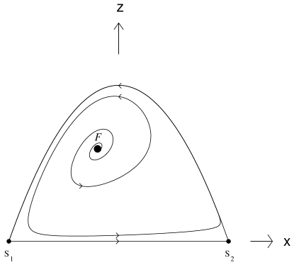
Figure 1: Phase portrait of the system (26)–(27), corresponding to the isotropic FRW model with $\Lambda_{\rm M}>0$. Equilibrium points are denoted by dots and the labels in all figures correspond to those equilibrium points (and hence the exact solutions they represent) discussed in the text. We shall adopt the convention throughout that large black dots represent sources (i.e., repellors), large grey-filled dots represent sinks (i.e., attractors), and small black dots represent saddles. Note that in this phase space orbits are future asymptotic to a heteroclinic cycle.

In the invariant set $1-x^{2}-z=0$, corresponding to the case of a zero axion field, Eqs. (26) and (27) reduce to the single ordinary differential equation:

$$\frac{dx}{d\Theta}=\frac{1}{2}\left(1-x^{2}\right)\left(x-\sqrt{3}\right),$$ (31)

which can be integrated to yield an exact solution in terms of $\Theta$–time.

IIIb Anisotropic Model for $\Lambda_{\rm M}>0$

In the full system (23)-(25), corresponding to the anisotropic model with a non–trivial shear parameter, there exists the isolated equilibrium point (and their associated eigenvalues)

$$F: x=-\frac{1}{3\sqrt{3}},\qquad y=0,\qquad z=\frac{16}{27}$$ (32)

$$\left(\lambda_{1},\lambda_{1},\lambda_{3}\right)=\left(\frac{1}{3}+\frac{i}{9}\sqrt{231},\frac{1}{3}-\frac{i}{9}\sqrt{231},\frac{4}{3}\right)$$

$$W: y=1-x^{2},\qquad z=0\qquad\mbox{($x$ arbitrary)}$$ (33)

$$\left(\lambda_{1},\lambda_{1},\lambda_{3}\right)=\left(-2\sqrt{3}\left[x+\frac{1}{\sqrt{3}}\right],\sqrt{3}\left[x-\frac{1}{\sqrt{3}}\right],0\right)$$

Hence, $F$ is a global source. The set $W$ lies in the invariant set $z=0$ on the boundary $y=1-x^{2}$. Points on $W$ with $x\in(-1/\sqrt{3},1/\sqrt{3})$ are local sinks, while the remaining points are saddles in the full three-dimensional phase space. (In the invariant set $z=0$ equilibrium points with $x\in[-1,-1/\sqrt{3})$ are repelling and those with $x\in(-1/\sqrt{3},1]$ are attracting). The phase portrait for this system is given in Fig. 2 and table 1 lists each equilibrium set and its stability..

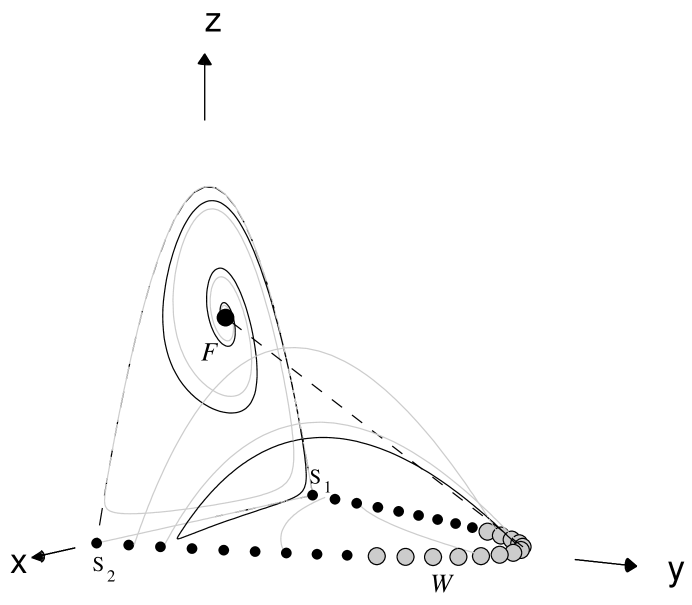
Figure 2: Phase portrait of the system (23)–(25) corresponding to the axisymmetric Bianchi type I cosmology with $\Lambda_{\rm M}>0$. Note that $W$ denotes a line of non–isolated equilibrium points. The dashed line represents the exact $x=\mbox{constant}$ solution (34)–(36). See caption to Fig. 1 for notation. Arrows on the trajectories in this three–dimensional phase space have been suppressed since the direction of increasing time is clear using this notation. Grey lines represent typical trajectories found within the two-dimensional invariant sets, dashed black lines are those trajectories along the intersection of the invariant sets, and solid black lines are typical trajectories within the full three-dimensional phase space.

Equilibrium Point	Stability
$F$:    Eq. (32)	Repellor (Source)
$W$:  Eq. (33)	Attractor (Sink) for $\frac{-1}{\sqrt{3}}<x<\frac{1}{\sqrt{3}}$
	Saddle otherwise

Table 1: Equilibrium sets for anisotropic model with $\Lambda_{\rm M}>0$, and their stability (the equations where each set is defined is also listed).

We note that there exists an exact, anisotropic solution of Eqs. (23)–(25), where

$$x=-\frac{1}{3\sqrt{3}}=\mbox{constant}$$ (34)

and

$$y=-\frac{13}{8}\left(z-\frac{16}{27}\right).$$ (35)

This implies that

$$\frac{dz}{d\Theta}=\frac{9}{4}z\left(z-\frac{16}{27}\right)$$ (36)

and Eq. (36) can be integrated explicitly in terms of $\Theta$–time.

In the following Section we determine the effects of a negative cosmological constant. This allows a direct comparison to be made with the $\Lambda_{\rm M}>0$ models considered above.

IV Negative Cosmological Constant

In the case where $\Lambda_{\rm M}<0$, the generalized Friedmann constraint equation (10) implies that

$$\psi^{2}-\Lambda_{\rm M}\geq 3h^{2}+6N^{2}\geq 0.$$ (37)

We may therefore normalize by employing the quantity $\sqrt{\psi^{2}-\Lambda_{\rm M}}$. Defining the new variables

$$u \equiv \frac{\sqrt{3}h}{\sqrt{\psi^{2}-\Lambda_{\rm M}}}$$ (38)

$$v \equiv \frac{\psi}{\sqrt{\psi^{2}-\Lambda_{\rm M}}}$$ (39)

$$w \equiv \frac{6N^{2}}{\psi^{2}-\Lambda_{\rm M}},$$ (40)

where $0\leq\{u^{2},v^{2},w\}\leq 1$, and the new time variable

$$\frac{d}{d\Xi}=\frac{1}{\sqrt{\psi^{2}-\Lambda_{\rm M}}}\frac{d}{d\theta}$$ (41)

implies that Eqs. (12)-(14) become

$$\frac{du}{d\Xi} = \frac{\sqrt{3}}{2}\left(1-u^{2}\right)\left(1-v^{2}\right)+\left(1-u^{2}-w\right)\left(\sqrt{3}+uv\right)$$ (42)

$$\frac{dv}{d\Xi} = -\frac{1}{2}\left(1-v^{2}\right)\left(1-2u^{2}-2w+\sqrt{3}uv\right)$$ (43)

$$\frac{dw}{d\Xi} = w\left[2v\left(1-u^{2}-w\right)-\sqrt{3}u\left(1-v^{2}\right)\right].$$ (44)

The phase space is bounded by the sets $v=\pm 1$ and $w=1-u^{2}$, where the latter corresponds to a zero axion field. The dynamics is determined by the fact that the right-hand side of Eq. (42) is positive definite so that $u$ is a monotonically increasing function.

IVa Isotropic Model for $\Lambda_{\rm M}<0$

In the invariant set $w=0$, corresponding to the isotropic FRW model $(\beta=0)$, the system (42)–(44) reduces to the following two-dimensional system:

$$\frac{du}{d\Xi} = \frac{1}{2}\left(1-u^{2}\right)\left(2uv+\sqrt{3}[3-v^{2}]\right)$$ (45)

$$\frac{dv}{d\Xi} = \frac{1}{2}\left(1-v^{2}\right)\left(2u^{2}-1-\sqrt{3}uv\right).$$ (46)

The lines $u^{2}=1$ and $v^{2}=1$ are invariant sets, containing four equilibrium points $S_{u,v}$. These points are all saddles and are located at the intersections of the lines. Their eigenvalues are given by

$$S_{1,1}: \lambda_{1}=\sqrt{3}-1,\quad\lambda_{2}=-2(\sqrt{3}+1)$$ (47)

$$S_{-1,1}: \lambda_{1}=2(\sqrt{3}-1),\quad\lambda_{2}=-(\sqrt{3}+1)$$ (48)

$$S_{1,-1}: \lambda_{1}=-2(\sqrt{3}-1),\quad\lambda_{2}=(\sqrt{3}+1)$$ (49)

$$S_{-1,-1}: \lambda_{1}=-(\sqrt{3}-1),\quad\lambda_{2}=2(\sqrt{3}+1).$$ (50)

The remaining two equilibrium points and their eigenvalues are

$$R:(u_{-},v_{-})=\left(-1,-\frac{1}{\sqrt{3}}\right) \lambda_{1}=\frac{1}{\sqrt{3}},\quad\lambda_{2}=\frac{10}{\sqrt{3}}$$ (51)

$$A:(u_{+},v_{+})=\left(1,\frac{1}{\sqrt{3}}\right) \lambda_{1}=-\frac{1}{\sqrt{3}},\quad\lambda_{2}=-\frac{10}{\sqrt{3}}.$$ (52)

Consequently, $R$ is a source and $A$ is a sink. Fig. 3 depicts the phase plane of the system (45)–(46).

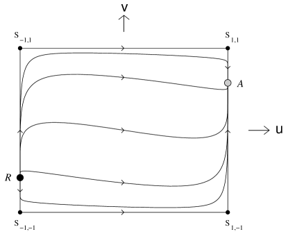
Figure 3: Phase portrait of the system (45)–(46) corresponding to the isotropic FRW model with $\Lambda_{\rm M}<0$. See caption to Fig. 1.

IVb Anisotropic Model for $\Lambda_{\rm M}<0$

In the full system (42)–(44) with a non-trivial shear parameter, the equilibrium points and their respective eigenvalues are:

$$W^{\pm}: v=\pm 1,u^{2}+w=1;$$ (53)

$$(\lambda_{1},\lambda_{2},\lambda_{3})=\left(0,\sqrt{3}\left[u\mp\frac{1}{\sqrt{3}}\right],-2\sqrt{3}\left[u\pm\frac{1}{\sqrt{3}}\right]\right)$$

$$R: v=-\frac{1}{\sqrt{3}},u=-1,w=0;$$ (54)

$$(\lambda_{1},\lambda_{2},\lambda_{3})=\frac{1}{\sqrt{3}}\left(1,2,10\right)$$

$$A: v=\frac{1}{\sqrt{3}},u=1,w=0;$$ (55)

$$(\lambda_{1},\lambda_{2},\lambda_{3})=-\frac{1}{\sqrt{3}}\left(1,2,10\right).$$

The saddle points $S_{\pm 1,-1}$ in subsection 4.1 are the endpoints to the line $W^{-}$. This line represents early–time attracting solutions for $-1/\sqrt{3}<u<1/\sqrt{3}$ and saddles otherwise. The saddle points $S_{\pm 1,1}$ are the endpoints to the line $W^{+}$. This corresponds to late–time attracting solutions for $-1/\sqrt{3}<u<1/\sqrt{3}$ and saddles otherwise. Hence, there are two early–time attractors given by the point $R$ and the line $W^{-}$ for $-1/\sqrt{3}<u<1/\sqrt{3}$. There are also two late–time attractors corresponding to the point $A$ and the line $W^{+}$ for $-1/\sqrt{3}<u<1/\sqrt{3}$. Fig. 4 depicts the three–dimensional phase space and table 2 lists each equilibrium set and its stability.

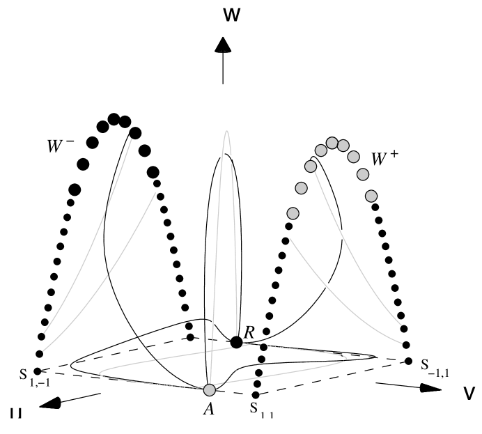
Figure 4: Phase portrait of the system (42)–(44) corresponding to the axisymmetric Bianchi type I model with $\Lambda_{\rm M}<0$. Note that $W^{\pm}$ denote lines of non-isolated equilibrium points. See captions to Figs. 1 and 2.

Equilibrium Point	Stability
$W^{-}$:  Eq. (53)	Repellor (Source) for $\frac{-1}{\sqrt{3}}<u<\frac{1}{\sqrt{3}}$
	Saddle otherwise
$W^{+}$:  Eq. (53)	Attractor (Sink) for $\frac{-1}{\sqrt{3}}<u<\frac{1}{\sqrt{3}}$
	Saddle otherwise
$R$:    Eq. (54)	Repellor (Source)
$A$:    Eq. (55)	Attractor (Sink)

Table 2: Equilibrium sets for anisotropic model with $\Lambda_{\rm M}<0$, and their stability (the equations where each set is defined is also listed).

This concludes the derivation of the phase portraits for the spatially flat and homogeneous cosmologies derived from Eq. (2). We proceed in the following Section to discuss their properties.

V Interpretation of the Phase Portraits

The dynamics of the isotropic cosmology described by the system (26)–(27) is of interest from a mathematical point of view due to the existence of the quasi–periodic behaviour. The orbits are future asymptotic to a heteroclinic cycle, consisting of the two saddle equilibrium points $S_{1}$ and $S_{2}$ and the single (boundary) orbits in the invariant sets $z=0$ and $1-x^{2}-z=0$ joining $S_{1}$ and $S_{2}$ (see Fig. 1). The former set corresponds to the zero $\Lambda_{\rm M}$ solution (given by Eqs. (15) with $q=0$) and the latter to the solution with constant axion field (see Eq. (31)); to our knowledge this exact solution was not previously known. In a given ‘cycle’, an orbit spends a long time close to $S_{1}$ and then moves quickly to $S_{2}$ shadowing the orbit in the invariant set $z=0$. It is then again quasi-stationary and remains close to the equilibrium point $S_{2}$ before quickly moving back to $S_{1}$ shadowing the orbit in the invariant set $1-x^{2}-z=0$. We stress that the motion is not periodic, and on each successive cycle a given orbit spends more and more time in the neighbourhood of the equilibrium points $S_{1}$ and $S_{2}$.

In Fig. 1, the exact solution corresponding to the equilibrium point $F$ is a power-law solution:

$$a = a_{*}(-t)^{1/3}$$

$$\Phi = \ln\left(\frac{16}{3\Lambda_{\rm M}}\right)-2\ln(-t)$$

$$\sigma = \sigma_{*}\pm\frac{\sqrt{15}\Lambda_{\rm M}}{16}(-t)^{2}$$

$$\dot{\beta} = 0,$$ (56)

where $t$ is defined over the range $-\infty<t<0$ by a suitable choice of an integration constant. This new solution represents a cosmology that collapses monotonically to zero volume at $t=0$. The curvature and coupling are both singular at this point. The universe is initially in a weak coupling regime, since $G_{\rm eff}\rightarrow 0$ as $t\rightarrow-\infty$, and the effective energy density of the axion field also vanishes in this limit.

All orbits in Fig. 1 begin at $F$. The cyclical nature of these orbits can be physically understood by reinterpreting the axion field in terms of a membrane. The homogeneity of the axion field, $\sigma=\sigma(t)$, implies that the two–form potential, $B_{\mu\nu}$, must be independent of cosmic time, and this in turn implies that its field strength must be proportional to the volume form of the three–space. If the topology of the spatial sections is given by a three–torus, $S^{1}\times S^{1}\times S^{1}$, the behaviour of the axion field is dynamically equivalent to that of a membrane that has been wrapped around this torus [16]. The collapse is resisted by this membrane and the universe undergoes a bounce. As the volume increases, however, the influence of the membrane is diminished, because the energy density of the axion is rapidly redshifted away. Consequently, the cosmological constant becomes important.

The subsequent effect of the cosmological constant can be determined by viewing Eq. (2) in terms of a Brans–Dicke action, where the dilaton–graviton coupling parameter is given by $\omega=-1$ [4]. The Brans–Dicke FRW models containing only a cosmological constant in the matter sector have been discussed previously by Barrow and Maeda, but their solutions only apply for $\omega>-5/6$ [7, 8]. The behaviour of the general solution for $\omega<-5/6$ is different and can be established by performing a conformal transformation to a frame where the dilaton field is minimally coupled to gravity. In such a frame the term containing $\Lambda_{\rm M}$ may be viewed as an exponential, self–interaction potential for the dilaton, where the exponent is uniquely determined by the value of $\omega$ [17]. When $\omega>-5/6$, the late–time attractor is a scaling solution, where the kinetic and potential energies of the dilaton field redshift in direct proportion [18]. For $\omega<-5/6$, however, the potential is so steep that the dilaton effectively becomes massless [19]. Thus, the late–time attractor when $\omega=-1$ corresponds to the solution (II) where $h_{*}^{2}=1/3$.

Further insight may be gained by defining new variables in the reduced action (4):

$$\chi\equiv 4\alpha-\Phi$$

$$\gamma\equiv\Phi-6\alpha$$

$$\tilde{t}=\int dte^{\varphi}.$$ (57)

In the case where $\dot{\beta}=\dot{\sigma}=0$, Eq. (4) reduces to

$$S=\int d\tilde{t}\left[-\frac{3}{2}\left(\frac{d\chi}{d\tilde{t}}\right)^{2}+\frac{1}{2}\left(\frac{d\gamma}{d\tilde{t}}\right)^{2}-\Lambda_{\rm M}e^{-\gamma}\right].$$ (58)

The momentum conjugate to the variable $\chi$ is constant, i.e., $d\chi/d\tilde{t}=C$, and the field equation for $\gamma$ is a Liouville equation:

$$\frac{d^{2}\gamma}{d\tilde{t}^{2}}=\Lambda_{\rm M}e^{-\gamma}.$$ (59)

The general solution to Eq. (59) satisfying the Hamiltonian constraint can be found. When $C>0$, it can be shown that $\gamma\propto\sqrt{3C^{2}}\tilde{t}$ in the late–time limit. Since the Hubble parameter is given by

$$\dot{\alpha}=-\frac{1}{2}e^{\varphi}\left(C+\frac{d\gamma}{d\tilde{t}}\right),$$ (60)

the late–time attractor corresponds to the collapsing solution in Eq. (II).

In effect, therefore, the cosmological constant resists the expansion and ultimately causes the universe to recollapse and asymptotically approach the saddle point $S_{1}$. On the other hand, the collapse causes the axion field to become relevant once more and a further bounce ensues. The process is then repeated with the universe undergoing a series of bounces. The orbits move progressively closer towards the two saddles, $S_{1,2}$, and spend increasingly more time near to these points. This behaviour is related to the fact that the kinetic energy of the shifted dilaton field increases monotonically with time, since Eq. (6) implies that $\ddot{\varphi}>0$.

When shear is included $(y\neq 0)$, $F$ still represents the only source in the system. The orbits follow cyclical trajectories in the neighbourhood of the invariant set $y=0$ and they spiral outwards monotonically, since Eq. (24) implies that $dy/d\Theta>0$. After a finite (but arbitrarily large) number of cycles the kinetic energy associated with the shear parameter, $\beta$, begins to dominate the axion and cosmological constant. The orbits then asymptote to the power-law solutions (II). All orbits in the full three-dimensional phase space actually spiral outwards around the orbit represented by the dashed line in Fig. 2 which corresponds to the exact solution (34)–(36) with $x={\rm constant}$. In terms of cosmic time, $t$, this exact solution satisfies

$$\Lambda_{\rm M}-\frac{16}{27}\psi^{2}+\frac{48}{13}N^{2}=0$$ (61)

and

$$\dot{\alpha}=-\frac{1}{9}\dot{\varphi},$$ (62)

whence from Eqs. (5)–(10) we obtain

$$\ddot{\varphi}=\dot{\varphi}^{2}+k_{\varphi}^{2}e^{2\varphi},$$ (63)

where $k_{\varphi}$ is an integration constant. Defining

$$\varrho\equiv\frac{e^{-\varphi}}{k_{\varphi}}$$ (64)

simplifies Eq. (63) to

$$\varrho\ddot{\varrho}=-1$$ (65)

and Eq. (65) can be integrated exactly to obtain $\dot{\varphi}$ [20]. A second integration then yields $\varphi$ in terms of the Inverse Error function, so that in principle we can obtain the scale factor as a function of time, $t$, from Eq. (62).

This cyclical behaviour does not arise if $\Lambda_{\rm M}<0$ (see Fig. 3). The equilibrium points $A$ and $R$ represent the power-law solutions:

$$a = \frac{a_{*}}{\sqrt{\pm\sqrt{-\frac{1}{2}\Lambda_{\rm M}}t}}$$

$$\Phi = \Phi_{*}-\ln\left[\pm\sqrt{-\frac{1}{2}\Lambda_{\rm M}}t\right]^{2}$$

$$\beta = \beta_{*}$$

$$\sigma = \sigma_{*},$$

where the $+$ sign corresponds to the point $R$ and the $-$ sign to the point $A$. Initially the universe is collapsing and the axion field induces a bounce, but this field can not dominate the dynamics again once the volume of the universe has increased sufficiently.

Fig. 4 depicts the axisymmetric Bianchi type I model when $\Lambda_{\rm M}<0$. In this phase space, for $-1/\sqrt{3}<u<1/\sqrt{3}$ the line $W^{-}$ represents the negative branch of the solution (II) for $h_{*}\in(-1/3,1/3)$. Likewise, for $-1/\sqrt{3}<u<1/\sqrt{3}$ the line $W^{+}$ represents the “$+$” solution in Eq. (II) for $h_{*}\in(-1/3,1/3)$. The four saddle points $S_{u,v}$ correspond to the power-law solutions (II) with $h_{*}=\pm 1/\sqrt{3}$. From Fig. 4 we see that generically trajectories asymptote away from either the line $W^{-}$ or the point $R$ and move towards the expanding power-law solutions $W^{+}$ or $A$. Hence, the cosmological constant is important in determining both the early– and late–time dynamics. Since $u$ is monotonically increasing (see (42)) we note that the occurrence of a bounce in these cosmological models is a typical feature.

VI Discussion

In this paper we have presented a qualitative analysis of spatially flat FRW and Bianchi type I cosmologies containing non–trivial dilaton and axion fields with a cosmological constant in the matter sector of the theory. The action we considered reduces to the string effective action when the cosmological constant vanishes. A complete stability analysis was performed in all cases by finding variables that led to a compactification of the phase space. We found that a cosmological constant has a significant effect on the dynamics of the string cosmologies (15).

One of the more interesting mathematical features of the models we have considered is the existence of quasi-periodic behaviour. This occurs in the isotropic cosmologies, where the orbits are future asymptotic to a heteroclinic cycle (see Fig. 1). The solutions interpolate between the saddles $S_{1}$ and $S_{2}$ corresponding to the power-law models (II) with $|h_{*}|=1/\sqrt{3}$. It would be interesting to consider the implications of this behaviour for the pre–big bang inflationary scenario [15]. We note that the phase portrait depicted in Fig. 1 is similar to that of Fig. 1(e) in [21] that describes the locally rotationally symmetric submanifold of the stationary Bianchi type I perfect fluid models in general relativity, although in this latter case the independent variable is space-like.

The general Bianchi cosmology, where the shear matrix is given by

$$\beta_{ab}={\rm diag}\left[\beta_{+}+\sqrt{3}\beta_{-},\beta_{+}-\sqrt{3}\beta_{-},-2\beta_{+}\right]$$ (67)

can be analysed directly by defining the variable $N$ in Eqs. (17) and (20) via $N^{2}=\sum_{i=\pm}N^{2}_{i}$. Orbits in the full phase space of Fig. 2 with non-trivial shear term (represented by the variable $y$) are repelled from the source $F$. The variable $y$ increases monotonically and the orbits spiral around the exact solution given by Eqs. (61)–(63), as represented by the dashed line in Fig. 2. (See also Fig. 1(f) and the Appendix in [21]). This implies that solutions are asymptotic in the past to the solution given by Eq. (V). At early times the orbits ‘shadow’ the orbits in the invariant set $y=0$ and undertake cycles between the saddles (in three-dimensional phase space) on the equilibrium set $W$ close to $S_{1}$ and $S_{2}$. These saddles on $W$ may be interpreted as Kasner–like solutions [21, 22]. Note that $y=0$ at $S_{1}$ and $S_{2}$, however, and there is no shear term in these cases. The orbits thus experience a finite number of cycles in which the solutions interpolate between different Kasner-like states. The orbits eventually asymptote towards a source on the line $W$.

This is perhaps reminiscent of the mixmaster behaviour that occurs in the Bianchi type VIII and IX cosmologies [22, 23]. These are the most general models in the Bianchi class A of spatially homogeneous universes [24]. In these models, Taub orbits joining equilibrium points of the Kasner set $K$ lead to the existence of infinite heteroclinic sequences which approximate the past asymptotic behaviour of generic orbits. (These heteroclinic sequences are defined by a map of $K$ onto itself). Mixmaster oscillations also occur in less general (i.e. lower–dimensional) Bianchi models with a magnetic field [25] or Yang-Mills fields [26]. It is interesting to note in the string context that mixmaster behaviour also occurs in scalar-tensor theories of gravity in general and in Brans-Dicke theory in particular [27].

This analogy is only suggestive. We note that if a non-zero central charge deficit is included, the quasi-periodic behaviour in the full (higher-dimensional) phase space does indeed persist [28]. Unlike the mixmaster oscillations, however, the orbits in Fig. 2 eventually spiral away from $y=0$, although there are orbits that experience a finite but arbitrarily large number of oscillations. However, it would be interesting to further explore any correspondence with possible mixmaster behaviour, particularly by including addtional anisotropic or matter degrees of freedom.

Some of the dynamics discussed in this paper is also relevant to higher–dimensional cosmological models. Kaluza-Klein compactification of ten–dimensional supergravity theories [2] onto an isotropic six-torus of radius $e^{\beta}$ introduces an additional modulus field into the effective four–dimensional action (1). Integration over the spatial variables for a spatially flat FRW model then leads to an action that is formally identical to that of Eq. (4) when we specify $\Lambda_{\rm M}=0$. In this sense, therefore, the action (4) can be recast into a higher–dimensional context, where the shear term $\beta$ plays the role of the modulus field and $\Lambda_{\rm M}$ is interpreted as a cosmological constant that is introduced after compactification.

More generally, type II supergravity theories contain Ramond–Ramond form–fields that do not couple directly to the dilaton field in the string frame [2]. Under dimensional reduction, these fields give rise to terms in the effective action of the form $Q^{2}\exp(c\beta)$, where $Q$ and $c$ are constants [29]; i.e., Ramond–Ramond charges give rise to exponential potentials for the modulus field rather than a simple constant term such as that considered in this work. However, from the analysis in section 3.1, there will be string solutions containing Ramond–Ramond fields that asymptote towards solutions with $\beta={\rm constant}$ ($y=0$ in Fig. 2), in which case $Q^{2}\exp(c\beta)$ is effectively constant. It might then be expected that the heteroclinic cycle that occurs in the invariant set $y=0$ (see Fig. 1) will play an important rôle in describing the dynamics of these string cosmologies.

Acknowledgments

We would like to thank Ulf Nilsson for helpful comments. APB is supported by Dalhousie University, AAC is supported by the Natural Sciences and Engineering Research Council of Canada (NSERC), and JEL is supported by the Royal Society.

References

References

- [1] E. S. Fradkin and A. Tseytlin, Phys. Lett. B158, 316 (1985); C. G. Callan, D. Friedan, E. J. Martinec, and M. J. Perry, Nucl. Phys. B262, 593 (1985); C. Lovelace, Nucl. Phys. B273, 413 (1986).
- [2] M. B. Green, J. H. Schwarz, and E. Witten, Superstring Theory (Cambridge University Press, Cambridge, 1987).
- [3] A. Shapere, S. Trivedi, and F. Wilczek, Mod. Phys. Lett. A6, 2677 (1991); A. Sen, Mod. Phys. Lett. A8, 2023 (1993).
- [4] C. Brans and R. H. Dicke, Phys. Rev. 124, 925 (1961).
- [5] E. J. Copeland, A. Lahiri, and D. Wands, Phys. Rev. D50, 4868 (1994); D51, 1569 (1995).
- [6] K. A. Meissner and G. Veneziano, Mod. Phys. Lett. A6, 3397 (1991).
- [7] J. D. Barrow and K. Maeda, Nucl. Phys. B341, 294 (1990).
- [8] J. E. Lidsey, Phys. Rev. D55, 3303 (1997).
- [9] D. S. Goldwirth and M. J. Perry, Phys. Rev. D49, 5019 (1993); K. Behrndt and S. Forste, Phys. Lett. B320, 253 (1994); Nucl. Phys. B430, 441 (1994).
- [10] N. Kaloper, R. Madden, and K. A. Olive, Nucl. Phys. B452, 677 (1995).
- [11] R. Easther, K. Maeda, and D. Wands, Phys. Rev. D53, 4247 (1996).
- [12] N. Kaloper, R. Madden, and K. A. Olive, Phys. Lett. B371, 34 (1996).
- [13] A. P. Billyard, A. A. Coley and J. E. Lidsey, .
- [14] M. P. Ryan and L. S. Shepley, Homogeneous Relativistic Cosmologies (Princeton Univ. Press, Princeton, 1975).
- [15] M. Gasperini and G. Veneziano, Astropart. Phys. 1, 317 (1992).
- [16] N. Kaloper, Phys. Rev. D55, 3394 (1997).
- [17] A. A. Coley, J. Ibáñez, and R. J. van den Hoogen, J. Math Phys. 38, 5256 (1997); A. P. Billyard, A. A. Coley, and J. Ibáñez, accepted to Phys. Rev. D, (1998).
- [18] A. R. Liddle, Phys. Lett. B220, 502 (1989).
- [19] J. E. Lidsey, Gen. Rel. Grav. 25, 399 (1993).
- [20] J. E. Lidsey and I. Waga, Phys. Rev. D51, 444 (1995).
- [21] U. S. Nilsson and C. Uggla, J. Math. Phys. 38, 2611 (1997).
- [22] J. Wainwright and G. F. R. Ellis, Dynamical Systems in Cosmology (Cambridge Univ. Press, Cambridge, 1997).
- [23] D. Hobill, A. Burd, and A. Coley, Deterministic Chaos in General Relativity (Plenum Press, New York, 1994).
- [24] G. F. R. Ellis and M. A. H. MacCallum, Commun. Math. Phys. 12, 108 (1969).
- [25] V. G. LeBlanc, D. Kerr, and J. Wainwright, Class. Quantum Grav. 12, 513 (1995).
- [26] J. D. Barrow and J. Levin, Phys. Rev. Lett. 80, 656 (1998).
- [27] R. Carretero-Gonzalez, H. N. Nunez-Yepez, and A. L. Salas Brito, Phys. Lett. A188, 48 (1994).
- [28] A. P. Billyard, Ph. D. thesis, Department of Physics, Dalhousie University, 1999.
- [29] J. Scherk and J. H. Schwarz, Nucl. Phys. 153, 61 (1979).