Late-Time Dynamics of Scalar Fields on Rotating Black Hole Backgrounds

Abstract

Motivated by results of recent analytic studies, we present a numerical investigation of the late-time dynamics of scalar test fields on Kerr backgrounds. We pay particular attention to the issue of mixing of different multipoles and their fall-off behavior at late times. Confining ourselves to the special case of axisymmetric modes with equatorial symmetry, we show that, in agreement with the results of previous work, the late-time behavior is dominated by the lowest allowed $l$-multipole. However the numerical results imply that, in general, the late-time fall-off of the dominating multipole is different from that in the Schwarzschild case, and seems to be incompatible with a result of a recently published analytic study.

The purpose of the studies presented in this paper is to point out the need for further work towards a definitive answer to the following question: How do perturbations of a rotating black hole get radiated away?

Using the Teukolsky formalism [1], we can search for an answer to that question by studying the evolution of a complex spin-weighted wavefunction that is defined in terms of curvature perturbations of a fixed black hole background geometry. The late-time dynamics of gravitational perturbations is governed by features very similar to those occurring for scalar test-fields [2, 6]. In the special case of vanishing spin-weight, the Teukolsky equation reduces to the linear wave equation for a scalar test field $\Phi$ on a Kerr background, which has a somewhat simpler structure than the Teukolsky equation. For the sake of simplicity, the present discussion is confined to the evolution of scalar test fields.

For a spherically symmetric, asymptotically flat background geometry, the angular variables can be separated off, and with an appropriate radial coordinate $x$ the wave equation for a scalar test field $\Phi$ reduces to a $(1+1)$ dimensional wave equation with an effective potential $V(x)$,

$$\left[\partial_{tt}-\partial_{xx}+V(x)\right]\Psi(t,x)=0\;.$$ (1)

When observed from a fixed location $x=R$, the dynamics of the wave consists of three stages (cf. Fig. 1): During the initial burst phase ($i$), the waveform is dominated by the initial data, in our case given by an outgoing pulse with compact support. The initial burst is followed by the exponentially damped quasinormal ringing ($ii$) and the so-called tail phase ($iii$), in which the amplitude of the field $\Phi$ falls off according to a power-law, $|\Phi|\propto t^{-\mu}$.

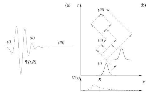
FIG. 1.: Wave propagation on a curved background: (a) Three stages of the dynamics: initial burst phase ($i$), quasinormal ringing ($ii$) and tail phase ($iii$). (b) The quasinormal ringing and the tail phase are understood in terms of scattering and interference – indicated by the dotted lines – of the wave off an effective potential $V(x)$, depicted by the dashed curve.

The discovery that waves propagating on a curved background die off in tails goes back to the original work by R. Price in the early 1970s [2]. In the special case of a background geometry given by a nonrotating black hole, and when the field is not initially static, the late time decay at a fixed location is given by $|\Phi|\propto t^{-(2l+3)}$, where $l$ is an angular separation parameter. In the last three decades, power-law tails on spherically symmetric backgrounds have been studied extensively by both analytic and numerical methods [3, 4, 5, 6, 7], not only at a fixed location (i.e. at timelike infinity), but also at the horizon of the black hole and at future null infinity.

This situation is in dramatic contrast to the case of a background given by a rotating Kerr black hole, in which until very recently no analytic predictions for the tail behavior were available. In fact it had been quite unclear whether tails are present at all, and, if they are, what the value of the power-law coefficient is. Numerical work, however, was done in an attempt to generalize the above results to the Kerr case [8]. Due to the breakdown of spherical symmetry of the background geometry, a multipole decomposition in terms of spherical harmonics loses its special meaning and it is no longer possible to expand $\Phi$ in spherical harmonics in the usual way. Although the functions $Y_{l}^{m}$ still form a complete set of functions for the description of a generic angular dependence, one now has to take into account the interaction between different $l$-multipoles in the course of the time evolution. Modes with different values of $m$, however, are not coupled because the background geometry is axisymmetric. Thus in order to take into account the contributions of all the different multipoles occurring in the numerical time evolution, only the azimuthal angular coordinate is separated off, and one has to solve a $(2+1)$ dimensional evolution problem for the field $\Psi$, defined by

$$\Phi\equiv\Psi(t,r^{*},\theta)e^{im\tilde{\phi}}\;,$$ (2)

where $r^{*}$ is the Kerr tortoise coordinate and $\tilde{\phi}$ is the azimuthal Kerr coordinate, that was chosen for technical reasons described in [8].

The main conclusion from the examples described in [8] can be stated in the following way: For a fixed value of the azimuthal separation parameter $m$, the late time dynamics is dominated by the lowest allowed $l$-multipole that is compatible with the choice of $m$ ($l$ has to satisfy the condition $l\geq m$) and with the equatorial symmetry properties of the initial data. Note that symmetric and antisymmetric modes do not get mixed during the evolution. The fall-off behavior of the dominating multipole is given by $|\Phi|\propto t^{-(2l+3)}$. This statement is illustrated in Fig. 2 by a specific example in which the initial pulse is given by $l=2,m=0$, which is not the lowest axisymmetric mode that is symmetric with respect to the equatorial plane: During the evolution there is a transition to the $l=m=0$ mode. The numerically determined power-law coefficient governing the decay of the $l=m=0$ mode is $\mu=3.15$ [9]. What, in this logarithmic diagram, appears to be a notch for angles smaller than $\theta\approx 0.9$, in fact represents the change of sign that the field $\Phi$ experiences for those angles during the transition from the initial $l=2$ distribution to the $l=0$ mode.

FIG. 2.: Plots of $|\Phi|$ for $m=0$, $a=0.9999$ for different angular directions $0\leq\theta\leq\pi/2$. The initial pulse was given by $l=2$. The time $t$ and $|\Phi|$ are shown on a logarithmic scale. For late times the numerically determined power-law coefficient is $\mu=3.15$.

The example shown in Fig. 2 illustrates the late-time behavior for one special choice of parameters. However there are several questions that remain open: What happens, for example, if we take initial data given by an $l=4$ multipole? In analogy to the situation depicted in Fig. 2, we expect a transition to the $l=0$ mode that will decay as $t^{-3}$. More generally, is seems obvious that any axisymmetric initial pulse with equatorial symmetry will descend to $l=0$ and that the late-time power-law decay of the field $\Phi$ will be given by $|\Phi|\propto t^{-3}$.

Recently, these and other issues have been addressed in two different analytic studies of late-time phenomena occurring in the course of the evolution of a massless scalar field on rotating black hole backgrounds.

L. Barack and A. Ori [10] have presented an analysis that is done in the time domain and yields expressions for the asymptotic behavior at future null infinity, at the black hole horizon, and at timelike infinity. After decomposing the field $\Phi$ into spherical harmonics,

$$\Phi=(r^{2}+a^{2})^{-1/2}\sum_{lm}\Psi^{lm}(t,r)Y_{l}^{m}(\theta,\phi)\;,$$

they consider an expansion of $\Psi^{lm}(t,r)$ in inverse powers of advanced time (late-time expansion). According to their prediction, to leading order in $t$, the late-time decay of a mode specified by $l$ and $m$ at timelike infinity is given by

$$\Phi\propto t^{-l-|m|-3-q}\;,$$ (3)

where $q=0$ if $l+m$ is even, and $q=1$ otherwise. Note that this prediction by Barack and Ori applies only in the case in which the $l=0$ mode is present in the initial data.

Independently, S. Hod has carried out an analysis that is based on a frequency decomposition of the scalar field $\Phi$ [11]. His analysis leads to the following conclusion for the late-time behavior at timelike infinity: The late-time behavior at timelike infinity is dominated by the lowest allowed multipole, $l=|m|$, if $l^{*}-|m|$ is even, and $l=|m|+1$ otherwise, where $l^{*}$ denotes the initial multipole. The late-time fall-off is given by

$$\Phi \propto t^{-l^{*}-|m|-p-1}\;\;\;\mbox{if}\;\;l^{*}\geq|m|+2\;,$$ (5)

$$\Phi \propto t^{-2l^{*}-3}\;\;\;\;\;\;\;\;\;\;\;\,\mbox{if}\;\;l^{*}=|m|,|m|+1\;,$$ (6)

where $p=0$ if $l^{*}-|m|$ is even, and $p=1$ otherwise.

For certain special choices of parameters, the expressions (3) and (2) are in agreement. Consider for example the case of an initial pulse given by $l=m=0$. Barack and Ori, as well as Hod, predict a late-time fall-off given by $|\Phi|\propto t^{-3}$. In this case both analytic predictions also agree with the numerical results, shown in [8].

In general, however, a comparison of the expressions (3) and (2) is made difficult by the fact that, as pointed out above, Eq. (3) does not allow a general statement about the dominating late-time behavior. In contrast to (3), Hod’s formula (2) makes a definite statement about the dominating late time decay, depending on the initial multipole. If one, for example, sets $m=0$ and chooses an initial pulse with $l^{*}=4$, Hod’s analysis implies $|\Phi|\propto t^{-5}$. According to Hod’s analysis, the $l=0$ multipole “remembers” the initial configuration $l^{*}$ in the sense that its decay rate does not depend only on the choice of $m$ and the equatorial symmetry properties of the initial data, but also on $l^{*}$.

The presence of two different analytic studies, one of which contains a rather surprising prediction, has motivated us to carry out a numerical investigation of the late time fall-off behavior.

For the axisymmetric evolution studies presented in this paper, we use the numerical $(2+1)$ evolution code from [8] with the black hole mass set to unity. We made several modifications to the previously used code. Instead of using the Boyer-Lindquist $\theta$ coordinate, we are using $y=-\cos\theta$, because this coordinate choice allows us to keep track of the behavior of the various angular modes more accurately. The $y$ derivatives of $\Psi$ are approximated using fourth order finite differences. We have used quadruple precision floating point arithmetic for the numerical computations, so that we can follow the dynamics up to late evolution times. This issue is not of importance for low initial multipoles, but for $l=4$ and higher it becomes relevant because of the steep fall-off at the beginning of the tail regime. The accuracy of the code was tested using standard convergence tests, based on numerical results obtained for short evolution times.

For $m=0$, in the $t,r^{*},y$ coordinates, the wave equation for $\Psi(t,r^{*},y)$ reads

$$\partial_{tt}\Psi-\frac{(r^{2}+a^{2})^{2}}{\Sigma^{2}}\partial_{r^{*}r^{*}}\Psi-\frac{\Delta(1-y^{2})}{\Sigma^{2}}\partial_{yy}\Psi$$ (7)

$$-\frac{2r\Delta}{\Sigma^{2}}\partial_{r^{*}}\Psi+\frac{2y\Delta}{\Sigma^{2}}\partial_{y}\Psi=0\;,$$ (8)

where we are using the standard abbreviations $\Delta\equiv r^{2}-2Mr+a^{2}$, and $\Sigma^{2}\equiv(r^{2}+a^{2})^{2}-a^{2}\Delta(1-y^{2})$ . The initial data are given by the Gaussian-like, initially outgoing pulse with compact support given by $50M\leq r^{*}\leq 150M$ used in [8].

The following figures represent an analysis of the data obtained from numerical evolutions. For a range of time parameter values $t$, the signal $\Psi$ at fixed radius is decomposed into angular modes. We start the evolutions with modes that are symmetric with respect to the equatorial plane ($l=0$ or $4$). Since symmetric modes do not get mixed with antisymmetric modes, we can discard the latter and just decompose the signal into even modes. Since we expect the signal at late times to be dominated by the lowest multipoles, we only take into account the three lowest even modes,

$$\Psi(t,r^{*}=\mbox{const.},y)=$$ (9)

$$\alpha(t)P_{0}(y)+\beta(t)P_{2}(y)+\gamma(t)P_{4}(y)\;,$$ (10)

where the $P_{0,2,4}(y)$ are the standard Legendre polynomials.

In Fig. 3 we depict the fall-off behavior of the absolute values of the expansion coefficients $|\alpha|$, $|\beta|$, and $|\gamma|$, extracted at $r^{*}=10$, as functions of the Boyer-Lindquist time $t$ for the test case $a=0$. The grid spacings are given by $dr^{*}=0.04$ and $dy=0.01$. The initial pulse is given by the $l=4$ multipole, and the computation is done with the same $(2+1)$ evolution code that is used in the $a\neq 0$ case. Since for $a=0$ the background is spherically symmetric, the $l=4$ multipole has to be preserved during the evolution. Hence we know that all contributions from modes other than $l=4$ are numerical artifacts. A least squares fit of a function $f(t)=c\,t^{-\mu}$ to $\gamma(t)$ yields the power-law $\gamma(t)=-3.33\times 10^{18}\,t^{-10.93}$. The power-law coefficient $\mu$ is within less than $0.7\%$ in agreement with the theoretical value of $\mu=11$. The expansion coefficients of the numerical contamination modes $l=0,2$ are orders of magnitude smaller than the $l=4$ mode, hence establishing the accuracy of the numerical evolution method.

FIG. 3.: Log-log plots of the coefficients $\alpha$, $\beta$, and $\gamma$ for $m=0$, $a=0$, evaluated at $r^{*}=10$. The initial data are given by an $l=4$ pulse. For late times, the decay of the $l=4$ mode is governed by the power-law $\gamma(t)\propto t^{-10.93}$.

What can we expect for $a\neq 0$? Intuitively we might anticipate a transition to the $l=0$ mode that will decay as $t^{-3}$, similar to the situation illustrated in Fig. 2. However we know that Hod’s analytic prediction, which we briefly discussed above, yields $|\Psi|\propto t^{-5}$ for the dominating $l=0$ mode at late times, contrary to a naive guess. For grid spacings given by $dr^{*}=0.04$ and $dy=0.01$, a fit to the numerically computed $\alpha(t)$ yields the power-law $\alpha(t)\propto t^{-6.04}$ for the decay of the $l=0$ mode which is dominating at late times. This result is deeply surprising. The transition to the $l=0$ mode is quite intuitive, but we might have expected a decay rate of $t^{-3}$, independently of the particular choice of the initial value of $l$, as long as the initial pulse is symmetric with respect to the equator. The numerical result is not only counter-intuitive, it also seems to be incompatible with the analytic prediction given in [11]. This suggests that the computed $\alpha(t)\propto t^{-6.04}$ behavior might represent a numerical artifact rather than a physically meaningful result.

FIG. 4.: Plots of $\mu_{\alpha}$ for $m=0$, $a=0.9999$, observed at $r^{*}=10$ (boxes) and $r^{*}=25$ (stars). The initial pulse was given by $l=4$.

This suspicion is confirmed by Fig. 4, that shows the grid size dependence of the numerically extracted power-law coefficient $\mu_{\alpha}$, that governs the decay of $\alpha$ at $r^{*}=10$ (boxes) and at $r^{*}=25$ (stars) The results were obtained from four runs with $dr^{*}=0.16,0.1,0.08,0.064$ and $dy=0.01,0.00625,0.005,0.004$, i.e. the discretization in the $y$ direction was chosen to be finer than in the cases above. To limit the computational expenses, the run times were shorter than in the previously considered cases, and $\mu_{\alpha}$ was extracted for $600<t<800$. As illustrated in Fig. 4, a fit of a function $\mu_{\alpha}=c_{1}+c_{2}\,dy^{c_{3}}$ to the numerical data yields a value of $c_{3}$ that is close to $4$, indicating that the discretization error is dominated by the finite difference approximation of the $y$ derivatives. The continuum limit of $\mu_{\alpha}$, however, seems to be neither $5$ nor $6$ and shows a rather weak dependence on the location of the observer, possibly a numerical artifact. Our numerical work strongly suggests that an extension of the existing analytic and numerical studies is necessary.

The studies presented in this paper show that, for $m$ set to zero and initial data with equatorial symmetry, the late-time behavior of scalar test fields on Kerr backgrounds is dominated by the lowest allowed $l$-multipole, namely $l=0$. The numerical results imply that, in general, the late-time fall-off of that dominating multipole is different from that in the Schwarzschild case, and appears not to agree with a central result of Hod’s recent analytic study [11]. Compatibility of our numerical results with the analysis of Ori and Barack [10], requires an extension of their studies to initial data that do not contain the $l=0$ multipole. The characterization that the initial pulse is “pure $l=4$” is ineluctably related to the use of the Boyer-Lindquist $\theta$ coordinate. Without explicit reference to the Boyer-Lindquist coordinate system, the numerical result can be stated as: There is an axisymmetric initial pulse with equatorial symmetry that exhibits a transition to $l=0$ and the late-time power-law decay of the field $\Phi$ is given by $|\Phi|\propto t^{-\mu}$, where the numerically determined power-law coefficient $\mu$ is different from the Schwarzschild value $\mu=3$. Additionally, our recent studies suggest that conclusions about the late-time power-law decay, made in [8] on the basis of particular examples, are not valid for generic situations.

The numerical results suggest that further analytic work is needed. It will also be useful to perform numerical computations up to later evolution times to underscore the validity of the statements made in this paper. Future numerical work should include studies of higher, non-axisymmetric multipoles, and also the physically relevant case of gravitational perturbations.

I am grateful to Amos Ori for originally suggesting this work to me. It is a pleasure to thank Richard H. Price for many encouraging discussions and helpful suggestions. I also wish to thank Pablo Laguna, Amos Ori, and Jorge Pullin for helpful discussions. This work was partially supported by NSF grant PHY-9734871. An allocation of computer time from the Center for High Performance Computing at the University of Utah is gratefully acknowledged. CHPC’s SGI Origin 2000 system is funded in part by the SGI Supercomputing Visualization Center Grant.

REFERENCES

- [1] S. A. Teukolsky, Phys. Rev. Lett. 29, 1114 (1972).
- [2] R. H. Price, Phys. Rev. D 5, 2419 (1972).
- [3] E. W. Leaver, Phys. Rev. D 34, 384 (1986).
- [4] C. Gundlach, R. H. Price, and J. Pullin, Phys. Rev. D 49, 883 (1994).
- [5] E. S. C. Ching, P. T. Leung, W. M. Suen, and K. Young, Phys. Rev. Lett. 74, 2414 (1995).
- [6] N. Andersson, Phys. Rev. D 55, 468 (1997).
- [7] L. Barack, Phys. Rev. D 59, 044017 (1999).
- [8] W. Krivan, P. Laguna, and P. Papadopoulos, Phys. Rev. D 54, 4728 (1996).
- [9] Please note that Fig. 6 from [8] should exhibit the same qualitative features as Fig. 2. As a careful error analysis in connection with the work published in this paper has shown, Fig. 6 in [8] does not correctly describe the transition from the to the multipole (due to a relatively coarse grid spacing in the Boyer-Lindquist coordinate).
- [10] L. Barack and A. Ori, Phys. Rev. Lett. 18, 4388 (1999).
- [11] S. Hod, Mode-Coupling in Rotating Gravitational Collapse of a Scalar Field, gr-qc/9902072.