Kerr-AdS and Kerr-dS solutions revisited

Abstract

We reconsider the Kerr metric with cosmological term $\Lambda$ imposing the condition that the angular velocity $\omega$ of the dragging of inertial frames vanishes at spatial boundaries. Some properties of the extreme black holes in the revisited solutions are discussed.

Dipartimento di Fisica dell’Università di Genova
Istituto Nazionale di Fisica Nucleare,Sezione di Genova
Via Dodecaneso 33, 16146 Genova, Italy

PACS numbers:   04.20.Jb , 97.60.Lf

With the advent of Maldacena’s conjecture of Anti de Sitter - Conformal Field Theory correspondence (AdS-CFT) [1], there has been a great deal of interest in studying the properties of black holes in AdS space [2-7], with special emphasis on the Kerr-AdS or Kerr-Newman-AdS solutions [8,9,10]. Rotating black holes in four dimensions with asymptotic AdS behavior were first constructed by Carter many years ago [11].

The purpose of this letter is to discuss various properties, which have not been considered in the literature before, of one of Carter’s families of Kerr vacuum solutions with cosmological term $\Lambda$. We refer to the stationary and axisymmetric metric (family $[A]$ of Ref.11) which can be written as

$$ds^{2}=\dfrac{\Delta_{r}}{\rho^{2}}\,\left[d\chi-\frac{a}{\Xi}\sin^{2}\vartheta d\psi\right]^{2}-\dfrac{\rho^{2}}{\Delta_{r}}\,dr^{2}\\ -\dfrac{\rho^{2}}{\Delta_{\vartheta}}\,d\vartheta^{2}-\dfrac{\sin^{2}\vartheta\Delta_{\vartheta}}{\rho^{2}}\,\left[ad\chi-\dfrac{(r^{2}+a^{2})}{\Xi}d\psi\right]^{2}$$ (1)

where

$$\begin{split}\rho^{2}&=r^{2}+a^{2}\cos^{2}\vartheta\\ \Delta_{r}&=-\dfrac{\Lambda}{3}r^{4}+(1-\dfrac{a^{2}\Lambda}{3})r^{2}-2Mr+a^{2}\\ \Delta_{\vartheta}&=1+\dfrac{a^{2}\Lambda}{3}\cos^{2}\vartheta\\ \Xi&=1+\dfrac{a^{2}\Lambda}{3}\end{split}$$ (2)

The parameter $M$ is related to the mass, $a$ to the angular momentum per unit mass while $\chi$ and $\psi$ are two ignorable coordinates. To express $\chi$ and $\psi$ by means of the usual time and azimuthal angle coordinates $t$ and $\varphi$, we use the coordinate transformations

$$\chi =\alpha\,t$$ (3)

$$\psi =\beta\,\varphi+\gamma\,t$$ (4)

where the constants $\alpha,\beta$ and $\gamma$ are to be determined with the conditions that the angular velocity $\omega$ of the dragging of inertial frames must vanish when $r$ reaches infinity if $\Lambda<0$ and when $r$ reaches the cosmological horizon if $\Lambda>0$ ; moreover $t$ and $\varphi$ will be properly normalized.

We first consider the Kerr-AdS case ($\Lambda<0$).

The required transformations are

$$\chi =\left(1+\dfrac{a^{2}\Lambda}{3}\right)^{2}t$$ (5)

$$\psi =\sqrt{1+\dfrac{a^{2}\Lambda}{3}}\,\varphi+\dfrac{a\Lambda}{3}\left(1+\dfrac{a^{2}\Lambda}{3}\right)t$$ (6)

and the corresponding line element (1) in Boyer-Lindquist coordinates becomes

$$ds^{2}=\dfrac{\left(1+\dfrac{a^{2}\Lambda}{3}\cos^{2}\vartheta\right)\left[\left(1+\dfrac{a^{2}\Lambda}{3}\cos^{2}\vartheta\right)\Delta_{r}-a^{2}\sin^{2}\vartheta\left(1-\,\dfrac{\Lambda r^{2}}{3}\right)^{2}\right]}{r^{2}+a^{2}\cos^{2}\vartheta}\,dt^{2}\\ {}\\ -\,\dfrac{r^{2}+a^{2}\cos^{2}\vartheta}{\Delta_{r}}\,dr^{2}-\,\frac{r^{2}+a^{2}\cos^{2}\vartheta}{1+\dfrac{a^{2}\Lambda}{3}\cos^{2}\vartheta}\,d\vartheta^{2}+\dfrac{4Mra\sin^{2}\vartheta\left(1+\dfrac{a^{2}\Lambda}{3}\cos^{2}\vartheta\right)}{\sqrt{1+\dfrac{a^{2}\Lambda}{3}}\,(r^{2}+a^{2}\cos^{2}\vartheta)}\,dtd\varphi\\ {}\\ -\,\dfrac{\sin^{2}\vartheta\left[\left(1+\dfrac{a^{2}\Lambda}{3}\cos^{2}\vartheta\right)(r^{2}+a^{2})^{2}-a^{2}\sin^{2}\vartheta\Delta_{r}\right]}{\left(1+\dfrac{a^{2}\Lambda}{3}\right)(r^{2}+a^{2}\cos^{2}\vartheta)}\,d\varphi^{2}$$ (7)

The solution is valid for $1+\dfrac{a^{2}\Lambda}{3}>0$ and becomes singular when the latter quantity is zero. The event horizon is located at $r=r_{+}$, the larger of the two positive roots $r_{+}$ and $r_{-}$ of the polynomial $\Delta_{r}$.

In this letter we limit ourselves to consider some properties of extreme black holes.

In the parameter plane   $(M^{2}\Lambda/3,a^{2}/M^{2})$  the curve $r_{+}=r_{-}$ represents the locus of the extreme black holes, i.e. the borderline between black holes and naked singularities. The equation of this curve is obtained requiring that $\Delta_{r}=\Delta_{r}^{\prime}=0$, where a prime denotes derivative with respect to $r$ and positive roots are to be considered. Putting for simplicity $x=M^{2}\Lambda/3,\;y=a^{2}/M^{2}$, one obtains the following equation

$$x^{3}y^{3}+9x^{2}y^{2}-9xy+27x-1-9x\,\sqrt{8y(xy-1)+9}\\ +(xy-1)^{2}\,\sqrt{xy(xy-14)+1}=0$$ (8)

The corresponding plot is given in Fig.1 and is comprised between the “critical” values $(-\,64/27,\,27/64)$ which correspond to $1+\dfrac{a^{2}\Lambda}{3}=0$, and the values $(0,1)$.

The angular velocity $\omega$ is given by

$$\omega=\dfrac{2Mra\,\sqrt{1+\dfrac{a^{2}\Lambda}{3}}\left(1+\dfrac{a^{2}\Lambda}{3}\cos^{2}\vartheta\right)}{\left(1+\dfrac{a^{2}\Lambda}{3}\cos^{2}\vartheta\right)(r^{2}+a^{2})^{2}-\,a^{2}\sin^{2}\vartheta\Delta_{r}}$$ (9)

One can immediately see that the angular velocity vanishes not only asymptotically, but also at the critical point above defined. A plot of $\omega$ as a function of the radius $r_{+}$ of the extreme black hole:

$$\omega=\dfrac{a\,\sqrt{1+\dfrac{a^{2}\Lambda}{3}}\left(1-\,\dfrac{\Lambda r_{+}^{2}}{3}\right)}{r_{+}^{2}+a^{2}}$$ (10)

is given in Fig.2, in terms of the dimensionless quantities $\omega^{\prime}=M\omega$ and $r_{+}^{\prime}=r_{+}/M$.

The area of the horizon is

$$A=4\pi\dfrac{r_{+}^{2}+a^{2}}{\sqrt{1+\dfrac{a^{2}\Lambda}{3}}}$$ (11)

It diverges at the critical point, gets its minimum near $r_{+}=M/2$ then increases till the value $8\pi M^{2}$ reached at $r_{+}=M$. A plot of $A$ as a function of $r_{+}$ is given in Fig.3, where are used the dimensionless quantities $A^{\prime}~{}=~{}A/(8\pi M^{2})$ and $r_{+}^{\prime}=r_{+}/M$. We notice that the minimum value of the area, which corresponds to the minimum value of the entropy, is also in correspondence with the maximum value of the angular velocity.

In a similar fashion we can now treat the Kerr-dS case ($\Lambda>0$).

The coordinate transformations are

$$\chi =\left(1+\dfrac{a^{2}\Lambda}{3}\right)t$$ (12)

$$\psi =\sqrt{1+\dfrac{a^{2}\Lambda}{3}}\,\varphi+\dfrac{a}{r_{c}^{2}+a^{2}}\left(1+\dfrac{a^{2}\Lambda}{3}\right)t$$ (13)

where $r_{c}$ represents the position of the cosmological horizon and is the largest of the three positive roots of the polynomial $\Delta_{r}$, the other two roots being still labelled by $r_{+}$ (the event horizon) and $r_{-}$ (the Cauchy horizon).

The line element (1) becomes

$$ds^{2}=\dfrac{(r_{c}^{2}+a^{2}\cos^{2}\vartheta)^{2}\Delta_{r}-a^{2}\sin^{2}\vartheta\left(1+\dfrac{a^{2}\Lambda}{3}\cos^{2}\vartheta\right)(r_{c}^{2}-r^{2})^{2}}{(r_{c}^{2}+a^{2})^{2}(r^{2}+a^{2}\cos^{2}\vartheta)}\\ {}\\ -\,\dfrac{r^{2}+a^{2}\cos^{2}\vartheta}{\Delta_{r}}\,dr^{2}-\,\frac{r^{2}+a^{2}\cos^{2}\vartheta}{1+\dfrac{a^{2}\Lambda}{3}\cos^{2}\vartheta}\,d\vartheta^{2}\\ {}\\ +\dfrac{2a\sin^{2}\vartheta\left[\left(1+\dfrac{a^{2}\Lambda}{3}\cos^{2}\vartheta\right)(r_{c}^{2}-r^{2})(r^{2}+a^{2})-\,(r_{c}^{2}+a^{2}\cos^{2}\vartheta)\Delta_{r}\right]}{\sqrt{1+\dfrac{a^{2}\Lambda}{3}}(r_{c}^{2}+a^{2})(r^{2}+a^{2}\cos^{2}\vartheta)}dtd\varphi\\ {}\\ -\,\dfrac{\sin^{2}\vartheta\left[\left(1+\dfrac{a^{2}\Lambda}{3}\cos^{2}\vartheta\right)(r^{2}+a^{2})^{2}-a^{2}\sin^{2}\vartheta\Delta_{r}\right]}{\left(1+\dfrac{a^{2}\Lambda}{3}\right)(r^{2}+a^{2}\cos^{2}\vartheta)}\,d\varphi^{2}$$ (14)

In this case the curve of the extreme black holes in the plane $(M^{2}\Lambda/3,\,a^{2}/M^{2})$, which is given again by Eq.($8$), begins at the point $(0,1)$ and ends at the point $\left(\dfrac{16}{135+78\sqrt{3}},\,\dfrac{3+2\sqrt{3}}{16}\right)$ where the three positive roots of the polynomial $\Delta_{r}$ have the same value equal to $\dfrac{(3+2\sqrt{3})M}{4}$; the corresponding plot is shown in Fig.1.

The angular velocity $\omega$ is given by

$$\omega=\dfrac{a\,\sqrt{1+\dfrac{a^{2}\Lambda}{3}}\left[\left(1+\dfrac{a^{2}\Lambda}{3}\cos^{2}\vartheta\right)(r_{c}^{2}-r^{2})(r^{2}+a^{2})-(r_{c}^{2}+\cos^{2}\vartheta)\Delta_{r}\right]}{(r_{c}^{2}+a^{2})\left[\left(1+\dfrac{a^{2}\Lambda}{3}\cos^{2}\vartheta\right)(r^{2}+a^{2})^{2}-a^{2}\sin^{2}\vartheta\Delta_{r}\right]}$$ (15)

and as requested goes to zero as $r\to r_{c}$ ; we notice that, as expected, also $g_{tt}$ goes to zero in this limit. A plot of $\omega$ as a function of $r_{+}$:

$$\omega=\dfrac{a(r_{c}^{2}-r_{+}^{2})\sqrt{1+\dfrac{a^{2}\Lambda}{3}}}{(r_{c}^{2}+a^{2})(r_{+}^{2}+a^{2})}$$ (16)

is given in Fig.2.

The area of the horizon can again be written as

$$A=4\pi\dfrac{r_{+}^{2}+a^{2}}{\sqrt{1+\dfrac{a^{2}\Lambda}{3}}}$$ (17)

The plot of $A$ as a function of $r_{+}$ is given in Fig.3 and shows that $A$ increases monotonously as $r_{+}$ goes from $M$ to $r_{c}$.

Some concluding remarks seem here appropriate.

a) While in the Kerr metric ($\Lambda=0$) the observer is put at infinity where $g_{tt}=1$, in the case $\Lambda\neq 0$ all the pairs $(r^{*},\vartheta^{*})$ solutions to $g_{tt}=1$ and fixing an observer should be considered. If then one wants to put the observer at a predefined position $(r_{0},\vartheta_{0})$ outside the ergosphere, it simply suffices to make the change of variable

$$t=\dfrac{\bar{t}}{\sqrt{g_{tt}(r_{0},\vartheta_{0})}}$$ (18)

which in turn modifies $\omega$ only by a scale factor.

b) If we consider, when $\Lambda<0$, the area of a surface at constant $t$ and $r$, and the lengths of the closed curves on it, we see that, while our coordinate transformations on $\psi$ and $\chi$ give asymptotically the correct value $2\pi r\sin\vartheta$ for a closed azimuthal curve at polar angle $\vartheta$, it is not possible to recover the asymptotically expected values $4\pi r^{2}$ and $2\pi r$ respectively for the area of a surface of radius $r$ and for the length of a polar curve $\varphi$ = constant. The drawback is due to the particular form of the term $\Delta_{\vartheta}$ which appears in the $g_{\vartheta\vartheta}$ component of the metric tensor. That term could be eliminated by the change of variable

$$\bar{\vartheta}=\int{\dfrac{d\vartheta}{\sqrt{\Delta_{\vartheta}}}}$$ (19)

but it would then be unpossible to express analytically $\vartheta$ as a function of $\bar{\vartheta}$. We notice however that in calculating areas related to black holes, as well as to extreme black holes as made here, the term $\Delta_{\vartheta}$ gets simplified in calculations by the use of the condition $\Delta_{r}=0$.

c) Finally, the fact that the Kerr-dS Universe is closed requires the presence of another antipodal mass $M$ equal to the mass of the original source and endowed with equal but opposite angular momentum.

Figure captions

Figure 1: The curve of the extreme black holes. Here $x=M^{2}\Lambda/3,\;y=a^{2}/M^{2}$. A dashed line separates the two regions where $\Lambda$ takes opposite signs.

Figure 2: The angular velocity $\omega^{\prime}$ as a function of $r_{+}^{\prime}$. The ordinate axis separates the regions where $\Lambda<0$ (left) and where $\Lambda>0$ (right).

Figure 3: The area $A^{\prime}$ as a function of $r_{+}^{\prime}$. The ordinate axis separates the regions where $\Lambda<0$ (left) and where $\Lambda>0$ (right).

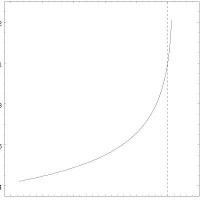
Figure 1: The curve of the extreme black holes. Here $x=M^{2}\Lambda/3,\;y=a^{2}/M^{2}$. A dashed line separates the two regions where $\Lambda$ takes opposite signs.

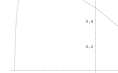
Figure 2: The angular velocity $\omega^{\prime}$ as a function of $r_{+}^{\prime}$. The ordinate axis separates the regions where $\Lambda<0$ (left) and where $\Lambda>0$ (right).

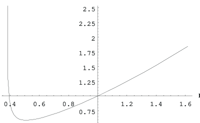
Figure 3: The area $A^{\prime}$ as a function of $r_{+}^{\prime}$. The ordinate axis separates the regions where $\Lambda<0$ (left) and where $\Lambda>0$ (right).

References

[1] Maldacena J M 1998 Adv. Theor. Math. Phys.2 231
[2] Åminneborg S, Bengtsson I, Holst S and Peldàn
P 1996 Class. Quantum Grav.13 2707
[3] Mann R B 1997 Class. Quantum Grav.14 L109;Mann R B and Smith W L 1997 Phys. Rev. D 56
4942
[4] Lemos J P S 1995 Class. Quantum Grav.12 1081;Lemos J P S and Zanchin V T 1996 Phys. Rev. D 54
3840
[5] Cai R G and Zhang Y Z 1996 Phys. Rev. D
54 4891
[6] Huang C G and Liang C B 1995 Phys. Lett. A
201 27
[7] Vanzo L 1997 Phys. Rev. D 56 6475
[8] Kostelecký V A and Perry M J 1996
Phys. Lett. B 371 191
[9] Caldarelli M M and Klemm D 1998 E-print
hep-th/9808097
[10] Hawking S W, Hunter C J and Taylor-Robinson M M 1999
Phys. Rev. D 59 064005
[11] Carter B 1968 Commun. Math. Phys.10 280