Curvature-induced phase transitions in the inflationary universe
- Supersymmetric Nambu-Jona-Lasinio Model
in de Sitter spacetime -

Abstract

The phase structure associated with the chiral symmetry is thoroughly investigated in de Sitter spacetime in the supersymmetric Nambu-Jona-Lasinio model with supersymmetry breaking terms. The argument is given in the three and four space-time dimensions in the leading order of the $1/N$ expansion and it is shown that the phase characteristics of the chiral symmetry is determined by the curvature of de Sitter spacetime. It is found that the symmetry breaking takes place as the first order as well as second order phase transition depending on the choice of the coupling constant and the parameter associated with the supersymmetry breaking term. The critical curves expressing the phase boundary are obtained. We also discuss the model in the context of the chaotic inflation scenario where topological defects (cosmic strings) develop during the inflation.

I Introduction

In the scenario of the early universe it is understood that the grand unified theory phase is broken down to the phase of quantum chromodynamics and electroweak theory through the Higgs mechanism. While Higgs fields are normally regarded as elementary fields, it is of interest to consider a possibility that the Higgs fields may be composed of some fundamental fermions as in the technicolor model and to see the consequence of this idea in the scenario of the early universe. On the other hand the supersymmetry is supposed to be a vital nature possessed by the fundamental unified theory and hence the incorporation of the supersymmetry in composite Higgs models is principally important. Under these circumstances it is natural for us to consider a supersymmetric composite Higgs model in the early stage of the universe and to see whether any remarkable effects are drawn during the inflation era.

The Nambu-Jona-Lasinio (NJL) model is a useful prototype model to investigate the mechanism of the dynamical symmetry breaking [1]. In many composite Higgs models the NJL-type Lagrangian is employed to realize the dynamical Higgs mechanism. From the standpoint of exploring the unified field theory of elementary particles it may be of interest to investigate a possibility of a supersymmetric version of the NJL model. Unfortunately, however, in the supersymmetric version of the NJL model the chiral symmetry is strongly protected to keep the boson-fermion symmetry and hence the dynamical chiral symmetry breaking does not take place [2]. If a soft supersymmetry breaking term is added to the supersymmetric NJL Lagrangian, the dynamical breakdown of the chiral symmetry is brought about for sufficiently large supersymmetry breaking parameter $\Delta$ [3]. The reason for this is simple: The large $\Delta$ implies the large effective mass of the scalar components of the superfields so that quantum effects due to the scalar components get suppressed compared with that of the spinor components. Thus the model becomes closer to the original NJL model which allows the dynamical fermion mass generation. Stating the same substance in a different way we realize that the boson by acquiring its mass term forces supersymmetry to make balance so that the fermion mass is generated dynamically.

The supersymmetric NJL model with soft supersymmetry breaking is useful to study the mechanism of the dynamical chiral symmetry breaking within the framework of supersymmetry. If we take the model seriously as a prototype of the unified field theory, it is natural to extend the argument to take into account circumstances of the finite temperature [4, 5] and spacetime-curvature as in the early universe [6, 7, 8].

At the inflation era the quantum effect of the gravitation is of minor importance while the external gravitational field is non-negligible. Hence we are naturally led to the supersymmetric NJL model in curved space. Dealing with the composite Higgs fields is essentially nonperturbative and does not accept approximate treatments. Accordingly we try to solve the problem rigorously working in a specific space-time, the de Sitter space, which possesses a maximal symmetry. The de Sitter space is suitable for describing the inflationary universe. As a nonperturbative method we rely on the $1/N$ expansion technique.

The four-fermion interaction model (which is the basis of the NJL model) in de Sitter space has been discussed by several authors [9, 10, 11, 12] and is found to reveal the restoration of the broken chiral symmetry for increasing curvature as a second order phase transition. The supersymmetric version of the NJL model in curved space was considered by I. L. Buchbinder, T. Inagaki and S. D. Odintsov [8] in the weak curvature limit. They found that the chiral symmetry is broken as the curvature increases. Their result is in contrast with the result in the nonsupersymmetric NJL model. On the other hand the supersymmetric NJL model in the flat space-time has been investigated by several authors [2] in the context of dynamical chiral symmetry breaking.

In the present paper we investigate the chiral symmetry breaking phenomena in the supersymmetric NJL model in de Sitter spacetime induced by the varying curvature. The situation is considered to be suitable to simulate the phase transition during the inflationary period. In the inflationary period the universe expands rapidly with increasing speed. This phenomenon is often called the de Sitter expansion. Many investigations on quantum phenomena in de Sitter spacetime have been performed motivated by the inflationary paradigm. The present authors have recently investigated the chiral symmetry breaking in the supersymmetric NJL model in de Sitter spacetime in ref. [6]. In ref. [6] we have mainly worked in the case of three spacetime dimensions. In the present paper we extend the previous investigation to the model of four spacetime dimensions, and discuss the cosmological consequence of the symmetry breaking phenomenon.

This paper is organized as follows: In section 2 we describe our model of the supersymmetric NJL model in de Sitter spacetime. Here formulae to obtain effective potentials in de Sitter spacetime in the 1/N expansion method is described. In section 3 we consider the case of three spacetime dimensions $D=3$. The results in section 3 partially overlap the ones in ref.[6]. We review the phase structure of the chiral symmetry because the case $D=3$ is very instructive for considering the case $D=4$. The case $D=4$ is investigated in section 4. In section 5 we consider our model in the context of the chaotic inflation and discuss the possible formation of cosmic strings during the inflation. Section 6 is devoted to the summary and discussions. In this paper we use the units $\hbar=k_{B}=c=1$, and adopt the convention $(-~{}+~{}+~{}+)$ for metric and curvature tensors [13].

II Supersymmetric Nambu-Jona-Lasinio Model in de Sitter Space

A Lagrangian for supersymmetric NJL

In this section we first summarize the basic ingredients of the supersymmetric NJL model in curved spacetime and then we evaluate the effective potential in de Sitter spacetime. We consider the following Lagrangian for the supersymmetric NJL model expressed in terms of the component fields of superfields [8],

$${\cal L} = -\nabla^{\mu}\phi^{{\dagger}}\nabla_{\mu}\phi-\rho^{2}\phi^{{\dagger}}\phi-\nabla^{\mu}\phi^{c{\dagger}}\nabla_{\mu}\phi^{c}-\rho^{2}\phi^{c{\dagger}}\phi^{c}$$ (2)

$$-\bar{\psi}(\not{\nabla}+\rho)\psi-\frac{N}{2\lambda}\rho^{2},$$

where $N$ is the number of components of boson field $\phi$ and fermion field $\psi$, respectively, $\lambda$ is the four-fermion coupling constant, and $\rho$ is the auxiliary field. Note that in Eq.(2) only relevant terms in the leading order of the $1/N$ expansion are exhibited.

Since the supersymmetry of the model protects the chiral symmetry from breaking [2], we introduce the following supersymmetry breaking terms,

$$\delta{\cal L}=-\Delta^{2}\phi^{\dagger}\phi-\Delta^{2}\phi^{c\dagger}\phi^{c}-\xi_{1}R\phi^{\dagger}\phi-\xi_{2}R\phi^{c\dagger}\phi^{c},$$ (3)

where $R$ is the spacetime curvature, and $\xi_{1}$, $\xi_{2}$, and $\Delta$ are coupling parameters, respectively.

B Calculation of effective potential

In this subsection we describe the effective potential in curved space. Our strategy is based on the $1/N$ expansion and we obtain the effective potential in the leading order of the expansion. The partition function for the Lagrangian $\cal L+\delta\cal L$ in $D$ spacetime dimension is given by

$$Z = {\cal N}\int{\cal D}\rho{\cal D}\phi{\cal D}\phi^{c}{\cal D}\psi{\cal D}\bar{\psi}\exp\Bigl{[}i\int d^{D}x\sqrt{-g}$$ (6)

$$\times\{\phi^{{\dagger}}(\nabla^{\mu}\nabla_{\mu}-\rho_{1}^{2})\phi+\phi^{c{\dagger}}(\nabla^{\mu}\nabla_{\mu}-\rho_{2}^{2})\phi^{c}$$

$$\hskip 28.45274pt-\bar{\psi}(\not{\nabla}+\rho)\psi-\frac{N}{2\lambda}\rho^{2}\}\Bigr{]},$$

up to the normalization constant, where $\rho_{1}$ and $\rho_{2}$ are defined by

$$\rho_{j}^{2}=\rho^{2}+\Delta^{2}+\xi_{j}R,$$ (7)

with $j=1,2$. Integrating over $\phi$, $\phi^{c}$, $\psi$, and $\bar{\psi}$, we find

$$Z = \int{\cal D}\rho[det(\nabla^{\mu}\nabla_{\mu}-\rho_{1}^{2})]^{-N}[det(\nabla^{\mu}\nabla_{\mu}-\rho_{2}^{2})]^{-N}$$ (9)

$$\times[det(\not{\nabla}+\rho)]^{N}\exp\Bigl{[}i\int d^{D}x\sqrt{-g}(-\frac{N}{2\lambda}\rho^{2})\Bigr{]}$$

$$= \int{\cal D}\rho\exp\Bigl{[}i\int d^{D}x\sqrt{-g}\Bigl{(}-\frac{N}{2\lambda}\rho^{2}\Bigr{)}$$ (13)

$$-N\ln det(\nabla^{\mu}\nabla_{\mu}-\rho^{2}-\Delta^{2}-\xi_{1}R)$$

$$-N\ln det(\nabla^{\mu}\nabla_{\mu}-\rho^{2}-\Delta^{2}-\xi_{2}R)$$

$$+N\ln det(\not{\nabla}+\rho)\Bigr{]}.$$

The effective action for Large $N$ is written as

$$\Gamma[\rho] = S_{eff}[\rho]+O(\frac{1}{N}),$$ (14)

and the effective potential $V(\rho)$ in the leading order of the $1/N$ expansion can be explicitly calculated such that

$$V(\rho) = -\frac{S_{eff}[\rho=\mbox{const}]}{\Omega}$$ (15)

$$= -\frac{1}{\Omega}\Bigl{[}\int d^{D}x\sqrt{-g}(-\frac{\rho^{2}}{2\lambda})$$ (19)

$$-i\ln\frac{det(\not{\nabla}+\rho)}{det(\not{\nabla})}$$

$$+i\ln\frac{det(\nabla^{\mu}\nabla_{\mu}-\rho^{2}-\Delta^{2}-\xi_{1}R)}{det(\nabla^{\mu}\nabla_{\mu}-\Delta^{2}-\xi_{1}R)}$$

$$+i\ln\frac{det(\nabla^{\mu}\nabla_{\mu}-\rho^{2}-\Delta^{2}-\xi_{2}R)}{det(\nabla^{\mu}\nabla_{\mu}-\Delta^{2}-\xi_{2}R)}\Bigr{]}$$

$$= -\frac{1}{\Omega}\Bigl{[}\int d^{D}x\sqrt{-g}(-\frac{\rho^{2}}{2\lambda})$$ (25)

$$-i\{Tr\ln(\not{\nabla}+\rho)-Tr\ln(\not{\nabla})\}$$

$$+i\{Tr\ln(\Box-\rho^{2}-\Delta^{2}-\xi_{1}R)$$

$$\hskip 28.45274pt-Tr\ln(\Box-\Delta^{2}-\xi_{1}R)\}$$

$$+i\{Tr\ln(\Box-\rho^{2}-\Delta^{2}-\xi_{2}R)$$

$$\hskip 28.45274pt-Tr\ln(\Box-\Delta^{2}-\xi_{2}R)\}\Bigr{]},$$

where $\Omega$ is the spacetime volume and $\Box$ denotes $\nabla^{\mu}\nabla_{\mu}$. The effective potential (25) is normalized so that $V(0)=0$. Eq.(25) may be rewritten in the form,

$$V(\rho) = \frac{\rho^{2}}{2\lambda}+i\int^{\rho}_{0}ds~{}tr\big{<}x|(\not{\nabla}+s)^{-1}|x\big{>}$$ (28)

$$+i\int^{\rho^{2}}_{0}dt~{}\big{<}x|(\Box-t-\Delta^{2}-\xi_{1}R)^{-1}|x\big{>}$$

$$+i\int^{\rho^{2}}_{0}dt~{}\big{<}x|(\Box-t-\Delta^{2}-\xi_{2}R)^{-1}|x\big{>}.$$

It is important to note that the last three terms on the right-hand side of Eq.(25) are related to the massive boson and fermion propagators $S(x,y;s)$ and $G(x,y;t)$. If we define the functions, $S(x,y;s)$ and $G(x,y;t)$, which satisfy

$$({\ooalign{\hfil/\hfil\crcr$\nabla$}}+s)S(x,y;s) = \frac{\delta^{(D)}(x,y)}{\sqrt{-g(x)}},$$ (31)

$$(\Box-t)G(x,y;t) = \frac{\delta^{(D)}(x,y)}{\sqrt{-g(x)}},$$ (32)

respectively, it is easy to find the relationship :

$$S(x,y;s) = \big{<}x|(\not{\nabla}+s)^{-1}|y\big{>},$$ (33)

$$G(x,y;t) = \big{<}x|(\Box-t)^{-1}|y\big{>},$$ (34)

by making use of the following equality

$$\int d^{D}x\sqrt{-g(x)}\;|x\big{>}\big{<}x|=\hat{\mbox{\boldmath{1}}},$$ (35)

$$\big{<}x|y\big{>}=\frac{\delta^{(D)}(x,y)}{\sqrt{-g(x)}}.$$ (36)

Thus the calculation of the effective potential in the leading order of the $1/N$ expansion reduces to the evaluation of the propagators in the de Sitter spacetime,

$$V(\rho) = {\rho^{2}\over 2\lambda}+i\int_{0}^{\rho}ds{\rm Tr}S(x,x;s)$$ (39)

$$+i\int_{0}^{\rho^{2}}dtG(x,x;t+\Delta^{2}+\xi_{1}R)~{}$$

$$+i\int_{0}^{\rho^{2}}dtG(x,x;t+\Delta^{2}+\xi_{2}R)~{}.$$

The next task is to write down the fermion and the boson propagators in de Sitter spacetime.

C Boson and fermion propagators in de Sitter spacetime

In this subsection we briefly review the boson and fermion propagators in de Sitter spacetime. The de Sitter spacetime is defined as the maximally symmetric curved spacetime. The quantum field theory in de Sitter spacetime has been studied extensively and the propagator for scalar fields is well-known [14, 15, 16, 17, 18]. The scalar propagator with mass squared $t$ in the D dimensional de Sitter spacetime is explicitly written as

$$G(x,y;t)=-i{r^{2-D}\over(4\pi)^{D/2}}{\Gamma({a_{\rm s}})\Gamma({b_{\rm s}})\over\Gamma({c_{\rm s}})}{}_{2}F_{1}({a_{\rm s}},{b_{\rm s}},{c_{\rm s}};1-z),$$ (40)

where $\Gamma(a)$ is the gamma faction, ${}_{2}F_{1}(a,b,c;1-z)$ is the hypergeometric function, and

$$a_{s}={1\over 2}\biggl{(}D-1+\sqrt{(D-1)^{2}-4tr^{2}}\biggr{)},$$ (41)

$$b_{s}={1\over 2}\biggl{(}D-1-\sqrt{(D-1)^{2}-4tr^{2}}\biggr{)},$$ (42)

$$c_{s}={D\over 2},$$ (43)

with

$$z={\sigma^{2}\over 2r^{2}},\hskip 28.45274pt\sigma^{2}={1\over 2}(\vec{x}-\vec{y})^{2}.$$ (44)

Note that $\sigma$ is in proportion to the geodesic distance between the two points $x$ and $y$, and $r$ is the radius of de Sitter space, which is related to the Hubble parameter by $H=1/r$. It should be emphasized that the non-minimal coupling term gives effective mass $D(D-1)\xi/r^{2}$, where $R=D(D-1)/r^{2}$.

The fermion propagator is written as [19, 20]

$$S(x,y;s)=\bigl{(}A(x,y;s)+B(x,y;s)\sigma_{;\mu}\gamma^{\mu}\bigr{)}U,$$ (45)

where U is the matrices composed of the Dirac matrices and

$$A(x,y;s) = i{sr^{2-D}\over(4\pi)^{D/2}}{\Gamma(a_{f})\Gamma(a_{f}^{*})\over\Gamma(c_{f})}$$ (47)

$$\times\sqrt{1-z}{}_{2}F_{1}(a_{f},a_{f}^{*},c_{f};1-z),$$

where

$$a_{f}={D\over 2}+isr,\hskip 14.22636ptc_{f}={D\over 2}+1.$$ (48)

We do not present the explicit expression of the invariant function $B(x,y;s)$ because it is irrelevant to our purpose of calculating the effective potential. In fact we find

$${\rm Tr}S(x,x;s) = \lim_{z\rightarrow 0}A(x,y;s){\rm Tr}U$$ (49)

$$= {\rm Tr}[1]\lim_{z\rightarrow 0}A(x,y;s),$$ (50)

with the normalization $\lim_{z\rightarrow 0}{\rm Tr}U={\rm Tr}[1]$.

Now we are ready to calculate the effective potential (39). It is instructive to investigate the case $D=3$ [6], because the effective potential can be written in terms of elementary functions. We first review the phase structure of the case $D=3$ in the next section, and then the case $D=4$ is studied in section 4.

III Analysis in $3$ Dimensions

A Gap Equation

Following the previous argument, the expression for the effective potential is given by

$$V(\rho) = {\rho^{2}\over 2\lambda}+i\int_{0}^{\rho}ds{\rm Tr}S(x,x;s)$$ (52)

$$+2i\int_{\Delta^{2}+\xi R}^{\Delta^{2}+\xi R+\rho^{2}}dtG(x,x;t)~{},$$

where we set $\xi_{1}=\xi_{2}=\xi$ for simplicity.

In order to write down the effective potential we consider the coincidence limit of the propagator, $lim_{y\rightarrow x}G(x,y;t)$. In the coincidence limit, the propagator diverges in general. Then we adopt the point splitting method and consider $G(x,y;t)$ around $z=0$. For that purpose we use the mathematical formula (e.g., [21]):

$${\Gamma(a)\Gamma(b)\over\Gamma(c)}{}_{2}F_{1}(a,b,c;1-z)=$$ (53)

$$\Gamma(a+b-c)z^{c-a-b}{}_{2}F_{1}(c-a,c-b,c-a-b+1;z)$$ (54)

$$+{\Gamma(a)\Gamma(b)\Gamma(c-a-b)\over\Gamma(c-a)\Gamma(c-b)}{}_{2}F_{1}(a,b,a+b-c+1;z)~{}.$$ (55)

With the use of this formula the boson propagator is written as

$$G(x,y;t)={-i\over 8\pi rz^{1/2}}+{i\over 4\pi r}\nu{\rm coth}\pi\nu+{\cal O}(z^{1/2})~{},$$ (56)

where we defined $\nu=\sqrt{tr^{2}-1}$. Analytic continuation is needed for $tr^{2}<1$. On the other hand for $z\rightarrow 0$ Eq.(47) reduces to

$$A(x,y;s) = {is\over 8\pi rz^{1/2}}-{is\over 4\pi r}\biggl{(}{1\over 4}+s^{2}r^{2}\biggr{)}{{\rm tanh}\pi sr\over sr}$$ (58)

$$+{\cal O}(z^{1/2})~{}.$$

Inserting (56) and (58) into (52), then the effective potential turns out to be,

$$V(\rho) = {\rho^{2}\over 2\lambda}+{1\over\pi r}\int_{0}^{\rho}dss\biggl{(}{1\over 4}+s^{2}r^{2}\biggr{)}{\tanh\pi sr\over sr}$$ (60)

$$-{1\over 2\pi r}\int_{\Delta^{2}+\xi R}^{\Delta^{2}+\xi R+\rho^{2}}dt\nu{\rm coth}\pi\nu,$$

where we have set ${\rm Tr}[1]=4$. Note that the divergent terms cancel each other, which would originate from the supersymmetry.

The gap equation, ${\partial V/\partial(\rho^{2})}=0$, reads

$${\pi r\over\lambda}+\biggl{(}{1\over 4}+\rho^{2}r^{2}\biggr{)}{\tanh\pi\rho r\over\rho r}$$ (61)

$$-\sqrt{\rho^{2}r^{2}+6\zeta-1}{\rm coth\pi\sqrt{\rho^{2}r^{2}+6\zeta-1}}=0~{},$$ (62)

where we defined

$$\zeta=\xi+{1\over 6}\Delta^{2}r^{2}.$$ (63)

Note that the solution of this gap equation is completely specified by two parameters $\zeta$ and $\pi r/\lambda$. This means that the phase structure derived from the effective potential is completely specified in the plane of these two parameters.

B Phase Structure

We present the typical shape of our effective potential in the case $D=3$ in Figure 1 (see also [6]). In the region labeled by ’S’, the effective potential behaves so that the symmetry is unbroken. In the region labeled by ’B’, the symmetry is broken through the second order phase transtion. Finally in the region labeled by ’F’, the symmetry is broken through the first order phase transtion. The boundaries in Fig. 1, which separate the phases, are obtained by direct observation of numetical analysis of the effective potential. Analytically the condition is described as follows. The solid line in Fig. 1 is found by solving

$${\partial V\over\partial(\rho^{2})}\Bigg{|}_{\rho=0}=0,$$ (64)

which is explicitely written as

$${\pi r\over\lambda}+{\pi\over 4}-\sqrt{6\zeta-1}\coth\pi\sqrt{6\zeta-1}=0.$$ (65)

On the other hand, the condition for the dashed line is rather complicated. The condition is $V(\rho_{*})=0$, where $\rho_{*}={\rm max}\{\rho_{1},\rho_{2}\}$ when the equation ${\partial V/\partial(\rho^{2})}=0$ has two different solutions $\rho_{1}$ and $\rho_{2}$.

The branching point in Fig. 1 is of special interest. It is a critical point which divides the broken phase into type ’F’ and type ’B’. At the branching point C the following conditions are found to be satisfied simultaneously:

$${\partial V\over\partial(\rho^{2})}\Bigg{|}_{\rho=0}=0,\ \ \ {\partial^{2}V\over\partial(\rho^{2})^{2}}\Bigg{|}_{\rho=0}=0.$$ (66)

The conditions are explicitly given respectively by Eq. (65) and

$$1-\frac{\pi^{2}}{12}+\frac{1}{2\sinh^{2}\pi\sqrt{6\zeta-1}}-\frac{\coth\pi\sqrt{6\zeta-1}}{2\pi\sqrt{6\zeta-1}}=0.$$ (67)

From Eq. (67) we find that $\zeta=0.290138(=:\zeta_{*})$ at the branching point. By substituting this value for $\zeta$ in Eq. (65) we obtain $\pi r/\lambda=0.08306$ at the branching point.

Since we have seen the phase structure of our effective potential, we now discuss the time-evolution of the chiral symmetry assuming an inflation background. This consideration will make sense if the Hubble parameter (radius of de Sitter spacetime) changes slowly and the effective potential in the inflation phase is well described by that in de Sitter spacetime found above. As we will see in section 5, the Hubble parameter slowly decreases as the universe evolves during the chaotic inflation in actual. And the curvature of de Sitter spacetime slowly decreases (radius $r$ increases).

First let us consider the case $\Delta=0$. In this case $\zeta$ is equal to $\xi$. If the coupling constant $\lambda$ and $\xi$ are fixed, we move from left to right by increasing $r$ in Fig. 1. This indicates that the chiral symmetry will be ultimately restored for sufficiently large $r$. The initial situation depends on the value of $\xi$. By direct observation of the gap equation one can easily show that if the parameter $\xi$ is kept below $1/4$ the effective potential stays in the region ’S’ in the limit of $\pi r/\lambda=0$. Thus the phase transition does not occur for $\xi<1/4$. On the other hand the effective potential is in a broken phase of type ’F’ or ’B’ if we take the value of $\xi$ above $1/4$. Then the phase restoration occurs as the curvature decreases.

Second we consider the case $\xi=0$ and $\Delta\neq 0$. In this case $\zeta=\Delta^{2}r^{2}/6$. If the coupling constant $\lambda$ and $\xi$ are fixed, then the trajectory for varying $r$ on the $(\zeta,\pi r/\lambda)$ plane will be the one as shown in Fig.2. By increasing the radius $r$, we move from the bottom to the top along the straight line. For each line, the value of $\Delta\lambda/\pi$ is fixed (a) $\Delta\lambda/\pi=100$, (b) $\Delta\lambda/\pi=15.9$, and (c) $\Delta\lambda/\pi=2$. Along the curve for $\Delta\lambda/\pi=100$ a first order phase transition occurs, however, a second order transition occurs for $\Delta\lambda/\pi=2$. The critical case is $\Delta\lambda/\pi=15.9$. For $\Delta\lambda/\pi<1$ the phase transition does not occur.

Thus in the model $\Delta\neq 0$ and $\xi=0$, the phase of the symmetry is in the symmetric phase first, and it is broken as the curvature of the universe decreases as long as $\Delta\lambda/\pi\geq 1$. On the other hand the symmetry is ultimately unbroken in the case $\Delta=0$. This case is not relevant to our conventional idea of symmetry breaking. Thus we focus our attention to the case $\Delta\neq 0$ and $\xi=0$ in the following arguments.

IV Analysis in 4 Dimensions

A Gap Equation

In this section we consider the case $D=4$. From Eq.(39) or (52) the gap equation, $\partial V/\partial(\rho^{2})=0$, reads,

$${1\over 2\lambda}+{i\over 2\rho}{\rm Tr}S(x,x;\rho)+2iG(x,x;\rho^{2}+\Delta^{2})=0.$$ (68)

Here we consider the case $\Delta\neq 0$ and $\xi_{1}=\xi_{2}=0$, because this choice of parameter is relevant to the conventional idea of symmetry breaking phenomena as described in section 3.

The boson propagators (40) in the case $D=4$ reduces to :

$$G(x,y;t)={-iH^{2}\over(4\pi)^{2}}{\Gamma({3/2}+\nu)\Gamma({3/2}-\nu)\over\Gamma(2)}$$ (69)

$$\hskip 28.45274pt\times{}_{2}F_{1}(3/2+\nu,3/2-\nu,2;1-z),$$ (70)

where we defined

$$\nu=\sqrt{{9\over 4}-{t\over H^{2}}-{\Delta^{2}\over H^{2}}}.$$ (71)

While the function $A$ of Eq.(47) is

$$A(x,y;s)={isH^{2}\over(4\pi)^{2}}{\Gamma(2+is/H)\Gamma(2-is/H)\over\Gamma(3)}$$ (72)

$$\hskip 28.45274pt\times\sqrt{1-z}{}_{2}F_{1}(2+is/H,2-is/H,3;1-z).$$ (73)

Since the propagators diverges in the coincidence limit, $z\rightarrow 0$, we adopt the point splitting regularization by keeping $z$ small but finite. In this case it is useful to use the mathematical formula (e.g., [21])

$${\Gamma(a)\Gamma(b)\over\Gamma(a+b-1)}{}_{2}F_{1}(a,b,a+b-1;1-z)=$$ (74)

$${1\over z}+(a-1)(b-1)\sum_{n=0}^{\infty}{(a)_{n}(b)_{n}\over n!(n+1)!}\Bigl{\{}\ln(z)+\psi(a+n)$$ (75)

$$\hskip 28.45274pt+\psi(b+n)-\psi(n+1)-\psi(n+2)\Bigr{\}}z^{n},$$ (76)

where $(a)_{n}=\Gamma(a+n)/\Gamma(a)$ and $\psi(x)$ is the polygamma function. With the use of this formula the gap equation reduces to

$${(2\pi/H)^{2}\over\lambda}+{1-\sqrt{1-z}\over z}$$ (77)

$$-\sqrt{1-z}(1+\rho^{2}/H^{2})\sum_{n=0}^{\infty}{(2+i\rho/H)_{n}(2-i\rho/H)_{n}\over n!(n+1)!}$$ (78)

$$\times\Bigl{\{}\ln(z)+\psi(2+i\rho/H+n)+\psi(2-i\rho/H+n)$$ (79)

$$\hskip 28.45274pt-\psi(n+1)-\psi(n+2)\Bigr{\}}z^{n}$$ (80)

$$+(-2+\rho^{2}/H^{2}+\Delta^{2}/H^{2})\sum_{n=0}^{\infty}{(3/2+\nu)_{n}(3/2-\nu)_{n}\over n!(n+1)!}$$ (81)

$$\times\Bigl{\{}\ln(z)+\psi(3/2+\nu+n)+\psi(3/2-\nu+n)$$ (82)

$$\hskip 28.45274pt-\psi(n+1)-\psi(n+2)\Bigr{\}}z^{n}=0.$$ (83)

The divergent terms of order ${\cal O}(z^{-1})$, which appears in the boson and fermion propagators, cancel each other in the effective potential. This would be traced back to the supersymmetry of the theory. However the logalithmic divergent terms ${\cal O}(\ln z)$ arise in the case $D=4$. Thus our theory depends on the cutoff parameter. Instead of $z$ we introduce the momentum cutoff parameter $\Lambda$. We can show that the geodesic distance $\sigma=(\vec{x}-\vec{y})^{2}/2$ is related to the momentum cutoff parameter $\Lambda$ such that $\sigma=\Lambda^{-2}$. Then we have the relation

$$z={H^{2}\over 2\Lambda^{2}},$$ (84)

where we used Eq.(44).

B Phase structure

Next we consider the phase structure of the model by solving the gap equation (83). Because of the complexity of equation, an analytic approach would not be useful in the case $D=4$. Then we adopt numerical method by calculating equation (83). As the gap equation depends on the cutoff parameter, we do not find a simple scaling relation in gap equation (83), on the contrast to the case $D=3$. Therefore we fix the cutoff parameter $\Lambda=10^{15}{\rm GeV}$ in the following arguments, for simplicity.

Fig. 3 shows the phase structure of the effective potential on the $(H/\Lambda,1/\lambda\Lambda^{2})$-plane. The curves in the figure show the phase boundary between a symmetric phase and a broken phase for $\Delta=$ $10^{15}{\rm GeV},~{}3\times 10^{14}{\rm GeV},~{}10^{14}{\rm GeV}$, respectively. In the right and upper region of each curve in Fig. 3, the effective potential behaves so that the symmetry is unbroken. On the other hand in the left and lower region of each curve the symmetry is broken. We discuss the type of the broken phase, i.e., first order or second order, in the later.

By decreasing the curvature (decreasing $H$) with the coupling constants, $\Lambda$, $\Delta$, and $\lambda$ fixed, we move from right to left in Fig. 3. This indicates that the effective potential is in the symmetric phase initially, however, the symmetry is broken as $H$ decreases if the coupling constant $\lambda$ is larger then a critical value. Let us find the critical value of the coupling constant, which depends on the supersymmetry breaking mass $\Delta$ and the cutoff parameter $\Lambda$. Taking the limit $H\rightarrow 0$ of Eq.(83), we find the following critical coupling constant $\lambda_{\rm cr}$,

$${1\over\lambda_{\rm cr}}=-{\Delta^{2}\over(2\pi)^{2}}\sum_{n=0}^{\infty}{1\over n!(n+1)!}$$ (85)

$$\times\biggl{[}\ln{\Delta^{2}\over 2\Lambda^{2}}--\psi(n+1)-\psi(n+2)\biggr{]}\bigg{(}{\Delta^{2}\over 2\Lambda^{2}}\biggr{)}^{n}.$$ (86)

We show the critical value $\lambda_{\rm cr}$ as a function of $\Delta/\Lambda$ in Fig. 4. We see the expected result in the figure that the critical coupling constant $\lambda_{\rm cr}$ must becomes larger as the the supersymmetry breaking mass $\Delta$ becomes smaller.

Finally in this section we discuss the effective potential of type of the first order phase transition. Similar to the case $D=3$ we find that the effective potential behaves so that the phase transtion occurs through first order transition for a specific range of coupling constants. The region is small and we can not recognize it in Fig. 3. Fig. 5 shows the region in Fig.3 under magnification for demonstraition, where we adopted the case $\Delta=10^{15}{\rm GeV}$. In the narrow region labeled by ’F’ the effective potential has the shape of the first order phase transition. For other cases, $\Delta=3\times 10^{14}{\rm GeV}$ and $\Delta=10^{14}{\rm GeV}$ in Fig. 3, we find narrow regions of ’F’ in a similar way. Thus the model for $D=4$ has the similar phase structure as the case $D=3$.

Because there appears many parameters in the case $D=4$ and we can not find a good scaling relation on the contrast to the case $D=3$. Due to this fact it is difficult to show the phase structure in case $D=4$ clearly. As will be discussed in the next section the change of the Hubble parameter is rather fast in the chaotic inflation model. Then the period that the the effective potential has the shape of the first order phase transition is very short compared with the Hubble expansion time. Then the cosmological importance of the first order transition is unclear at present. Therefore we only focus on the epoch of the (second or first) phase transtion in the inflationary universe and discuss other cosmological consequences because phase transitions in the universe predicts topological defects in general.

V Epoch of phase transtion in the chaotic inflationary model

In this section we consider a cosmological application of our model in the chaotic inflation universe [22]. Cosmological phase transition predicts the formation of topological defects in general. In our model $U(1)$ chiral symmetry is broken down and the formation of cosmic strings would be predicted by the phase transtion. In general topological defects are harmful, as examplified by the monopole problem and domain wall problem. However, cosmic strings have been studied with the motivation of the cosmic structure formation. The observational confrontation of the cosmic string scenario is still at issue[23].

The investigations in the present paper show that the symmetry breaking may occur during inflation era, which is triggered by the change of the curvature of spacetime. As an application we consider the phase transition in the context of the chaotic inflation model and the formation of the cosmic strings during the inflation. If the inflation lasts sufficiently long after the phase transition, the defects will be diluted. However, if the phase transition occurs at a suitable epoch of inflation, the dilution of the strings is not completed. Similar investigations were given on the basis of a simple model of curvature induced phase transition [24, 25]. Following their consideration we here discuss the epoch of the formation of the cosmic strings in our model during the chaotic inflation era.

We assume the chaotic inflation background. To be specific we assume that the inflation is derived by the field $\phi$ with the Lagrangian

$${\cal L}_{\phi}=-\nabla^{\mu}\phi\nabla_{\mu}\phi-{1\over 2}m^{2}\phi^{2}.$$ (87)

Here we set $m=10^{13}{\rm GeV}$ [25], which is the constraint from the amplitude of density perturbations for a successful inflation scenario. With the background metric,

$$ds^{2}=-dt^{2}+a(t)^{2}d{\bf x}^{2},$$ (88)

the equations of motion under the slow roll approximation take the form,

$$3H\dot{\phi}+m^{2}\phi=0,$$ (89)

$$H^{2}={4\pi\over 3M_{\rm PL}^{2}}{m^{2}\phi^{2}},$$ (90)

where $H=\dot{a}/a$ is the hubble parameter, and the dot denotes (cosmic time) $t$ differentiation. The solution of inflation is well known

$$\phi(t)=\phi_{i}-{mM_{\rm PL}\over 2\sqrt{3\pi}}(t-t_{i}),$$ (91)

$$a(t)=a_{i}\exp\Biggl{[}{2\pi\over M_{\rm PL}^{2}}(\phi_{i}^{2}-\phi(t)^{2})\Biggr{]},$$ (92)

$$H(t)=\sqrt{4\pi m^{2}\over 3M_{\rm PL}^{2}}\phi(t),$$ (93)

$$R=12H^{2}+6\dot{H}={16\pi\over M_{\rm PL}^{2}}m^{2}\phi^{2}(t)-2m^{2}$$ (94)

$$\hskip 11.38092pt\simeq{16\pi\over M_{\rm PL}^{2}}m^{2}\phi^{2}(t),$$ (95)

where $M_{\rm PL}$ is the Plank mass, and the subscript ‘i’ denotes the value at the initial time when the inflation started.

In this chaotic inflation model the horizon crossing (during the inflation) of the fluctuation of the wave length corresponding to the present horizon size occurs at $\phi(t)\sim 3M_{\rm PL}$. The epoch of forming cosmic string are estimated as follows. The phase of $\rho$ does not fix soon after the phase transition because of the quantum fluctuations of the $\rho$ field. Following the previous investigations on curvature induced phase transition [24, 25, 22], the phase of $\rho$ fixes at the time, when the condition is satisfied

$$H^{2}=-\lim_{\rho\rightarrow 0}V(\rho)^{\prime\prime}~{},$$ (96)

which we may regard as the time of the string formation during the inflation. We denote the value of $\phi(t)$ at this time as $\phi_{2}$. With the use of equation (90), $\phi_{2}$ is written as

$$\phi_{2}=\sqrt{-{3M_{\rm PL}^{2}\over 4\pi m^{2}}\lim_{\rho\rightarrow 0}V(\rho)^{\prime\prime}}.$$ (97)

In the previous work [24, 25] the formation of the cosmic strings during inflation was discussed to avoid observational difficulties of the cosmic string scenario. They argued the range of the model parameter (coupling constant) to realize the suitable formation of the cosmic strings. In this paper we consider the observational possibility and find the condition that the cosmic strings are formed during the inflation without complete dilution of the cosmic strings so that the cosmic strings may exist in the universe at present time. The condition is simply given by

$${M_{\rm PL}\over\sqrt{4\pi}}\lower 2.15277pt\hbox{$\;\buildrel<\over{\sim}\;$}\phi_{2}\lower 2.15277pt\hbox{$\;\buildrel<\over{\sim}\;$}{3M_{\rm PL}},$$ (98)

where we have assumed that the strings are formed at the rate of one string per horizon volume at the formation epoch.

This condition constrains the coupling constant $\lambda$ in our model. From Eq.(96), we have

$${1\over\lambda}+H^{2}-{H^{2}\over(2\pi)^{2}}\sqrt{1-z}{}_{2}F_{1}(2,2,3;1-z)$$ (99)

$$+{H^{2}\over(2\pi)^{2}}{\pi(1/4-\mu^{2})\over\cos\pi\mu}{}_{2}F_{1}(3/2+\mu,3/2-\mu,2;1-z)=0,$$ (100)

where $\mu=\sqrt{9/4-\Delta^{2}/H^{2}}$, $z=H^{2}/2\Lambda^{2}$, and $H$ is specified as

$$H=\sqrt{4\pi m^{2}\over 3M_{\rm PL}^{2}}\phi_{2}.$$ (102)

Fig.6 shows the formation time of the cosmic strings on the parameter space, $\lambda$ and $\Delta$. Here we set $\Lambda=10^{15}{\rm GeV}$. The result depends on the choice of cutoff parameter $\Lambda$. However the qualitative feature does not depend on the choice of $\Lambda$. The region between the two solid curves in Fig.6 satisfies the condition (98). The lower solid curve is from the condition that the formation of the strings occurs at $\phi_{2}=3M_{\rm PL}$. While the upper solid curve comes from $\phi_{2}=M_{\rm PL}/\sqrt{4\pi}$. The larger coupling constant $\lambda$ leads to the earlier formation of the strings during the inflation. And the larger breaking parameter $\Delta$ also leads to the earlier formation of the strings. Fig.6 shows this expected result. Thus if we make a choice of parameters in the lower region than the lower solid curve, the strings are diluted out by the inflation and they would not be observable. The dashed line, which is almost overlapped with the upper solid line, shows the critical coupling constant for the phase transitions (see also Fig. 4). Therefore the strings do not form when we make a choice of parameters in the region above the dashed line.

VI Conclusions

In summary we have shown that the curvature of spacetime might be a trigger of phase transition during the inflation in a class of model of the dynamical symmetry breaking. To be specific we have investigated the phase structure of the supersymmetric NJL-model in de Sitter spacetime. By evaluating the effective potential in the leading order of the $1/N$ expansion, we have examined the phase structure of the chiral symmetry in three- and four-spacetime dimensions. We have investigated how the curvature of de Sitter spacetime changes the phase structure, and we have found that the symmetry breaking takes places as the first order as well as second order phase transition depending on the coupling constant and the parameter of the supersymmetry breaking in both cases of three- and four-spacetime dimensions.

In the case of three-spacetime dimensions, the gap equation reduces to a simple equation written by elementary functions. Divergent terms cancel each other and we do not need introduce a cutoff parameter. As shown in section 3, the shape of the effective potential can be specified by the two parameters, $r/\lambda$ and $\zeta$, which characterizes the phase structure. This model might not have physical meaning, however, it is very instructive to consider the case of four-spacetime dimensions.

In the case of four-spacetime dimensions, the gap equation does not reduce to a simple form, which is written by the hypergeometric functions. We have to introduce a (momentum) cutoff parameter to regularize the theory. The analysis is tedious, however, we have found that the phase structure is very similar to the case of three-spacetime dimensions. Similar to the case of three-spacetime dimensions we find a narrow region in which the effective potential has a shape of first order phase transitions. In the open inflation scenario a bubble nucleation (first order transition) occurs during the inflation [26]. It may be of interest to consider the possibility whether our model works as a successful model for the open universe or not. However this first order phase transition would not work successfully, because the curvature (Hubble parameter) of de Sitter spacetime changes rather fast during the inflation as we have shown in section 5.

We have briefly discussed a cosmological application in section 5. We consider the phase transition in the chaotic inflation background, neglecting the back-reaction from the fields which derives the phase transition. The strong coupling constant $\lambda$ leads to the early phase transition and the subsequent inflation dilute the strings. The weak coupling constant does not lead to the phase transition during the inflation. Thus this model may work as a model of forming the cosmic strings during the inflation if we choose the parameters in a suitable range [24, 25].

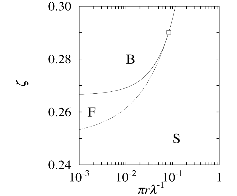
FIG. 1.: Phase structure of the model for $D=3$ on the $(\pi r/\lambda,\zeta)$ plane. In the regions labeled by ’S’, ’B’, and ’F’, the shape of the effective potential is of type of unbroken symmetry, of second order phase transtion, and of first order phase transition, respectively. The square denotes the branching point.

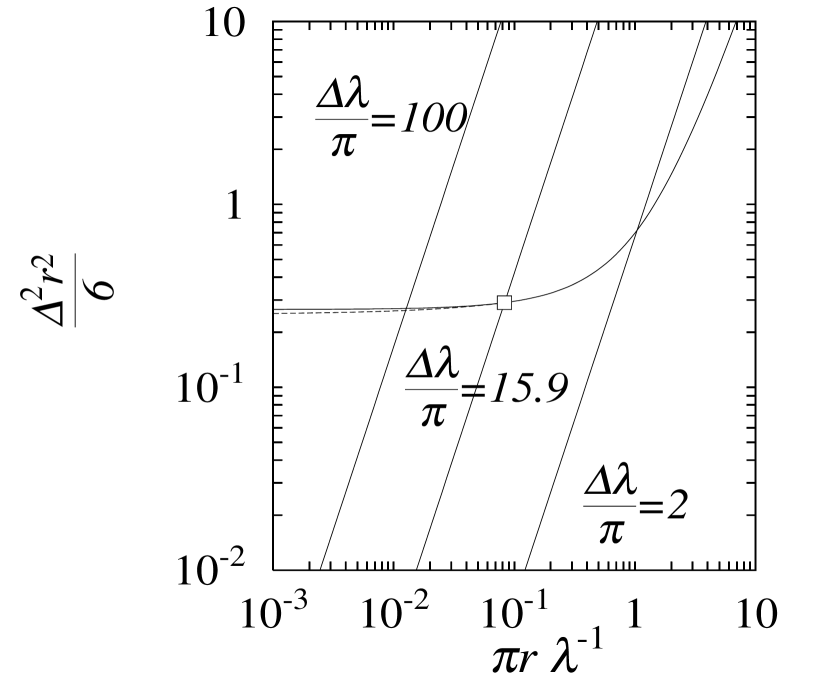
FIG. 2.: Typical trajectories for varying $r$ with $\Delta\lambda/\pi$ fixed on the $(\pi r/\lambda,\zeta)$ plane. We chose $\Delta\lambda/\pi=100$,  $15.9$, and $2$ for straight lines, respectively.

FIG. 3.: Phase boundary in the case $D=4$ on the $(H/\Lambda,1/\lambda\Lambda^{2})$ plane. Here $\Lambda=10^{15}{\rm GeV}$ is used. We adopted the supersymmetry breaking parameter $\Delta=10^{15},~{}3\times 10^{14},~{}10^{14}({\rm GeV})$, respectively, for each curve in the figure. The right and upper region labeled by ’S’ is in a symmetric phase for each curve. While the left and lower region labeled by ’B’ is in a broken symmetry.

FIG. 4.: Critical coupling constant $\lambda_{\rm cr}^{-1}\Lambda^{-2}$ of equation (4.8) as a function of $\Delta/\Lambda$.

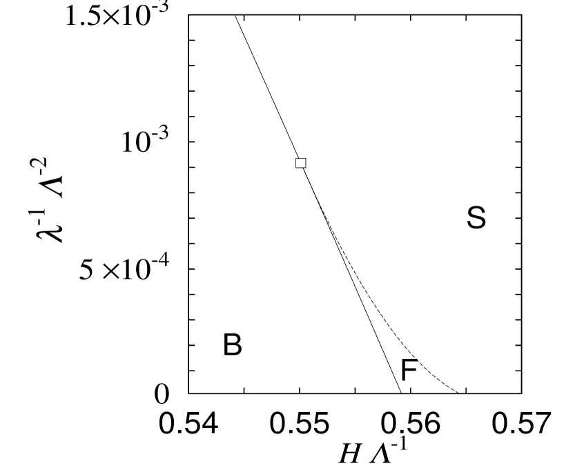
FIG. 5.: Phase boundary for the model for $D=4$ on the $(H/\Lambda,1/\lambda\Lambda^{2})$ plane. Here we set $\Lambda=10^{15}{\rm GeV}$ and $\Delta=10^{15}{\rm GeV}$. In the narrow region between two curves labeled by $F$, the effective potential has a shape of type of first order transition. The square is the branching point obtained from numerical calculation.

FIG. 6.: Constraint on formation epoch of cosmic strings on the $(1/\lambda$, $\Delta)$ plane. Here we adopted the momentum cutoff $\Lambda=10^{15}{\rm GeV}$. The upper solid curve reflects the condition $\phi_{2}=(4\pi)^{-1/2}M_{\rm PL}$ and the lower solid curve corresponds to $\phi_{2}=3M_{\rm PL}$. The dashed line shows the critical coupling constant $\lambda_{\rm cr}$.

- [1] Y.Nambu and G.Jona-Lasinio, Phys. Rev. 122, 345 (1961).
- [2] W. Buchmueller and S. T. Love, Nucl. Phys. B204 213 (1982); V. Elias, D. G. C. Mckeon, V. A. Miransky and I. A. Shovkovy, Phys. Rev. D54 7884 (1996); L. L. Buchbinder, T. Inagaki and S. D. Odintsov, Mod. Phys. Lett. A12 2271 (1997).
- [3] W. Buchmueller and U. Ellwanger, Nucl. Phys. B245 237 (1984).
- [4] J.Hashida, T.Muta and K.Ohkura, Mod. Phys. Lett. A13, 1235 (1998)
- [5] J.Hashida, T.Muta and K.Ohkura, Phys.Lett.B, in press (1999)
- [6] J. Hashida, S. Mukaigawa, T. Muta, and K. Ohkura, K. Yamamoto, Phys. Rev. D59, 101302 (1999).
- [7] T.Inagaki, T.Muta, and S. D. Odintsov, Prog. of Theor. Phys. Suppl. 127 93 (1997).
- [8] I. L. Buchbinder, T. Inagaki, and S. D. Odintsov, Mod. Phys. Lett. A12 2271 (1997).
- [9] H. Itoyama, Prog. Theor. Phys. 64, 1886 (1980).
- [10] I. L. Buchbinder and E. N. Kirillova, Int. J. Mod. Phys. A4, 143 (1989).
- [11] T.Inagaki, S.Mukaigawa, and T.Muta, Phys.Rev.D54, R4267 (1995).
- [12] E. Elizalde, S. Leseduarte, S. D. Odintsov and Yu. I. Shil’nov, Phys. Rev. D53, 1917 (1996).
- [13] C.W.Mister, K.S.Thone, and J.A.Wheeler, Gravitation (Freeman, San Francisco, 1973).
- [14] N. D. Birrell and P. C. W. Davies, Quantum Fields in Curved Space (Cambridge University Press, 1982).
- [15] T.S.Bunch and P. C. W. Davies, Proc.Roy.Soc.(London) A360, 117 (1978).
- [16] B. Allen, Phys. Rev. D32, 3136 (1985).
- [17] B. Allen and T. Jacobson, Commun. Math. Phys. 103 669 (1986).
- [18] E. A. Tagirov, Ann.Phys. (N.Y.)76, 561 (1973).
- [19] S. Mukaigawa, in preparation.
- [20] R. Camporesi, Comm. Math. Phys. 148, 283 (1992).
- [21] W.Magnus, F.Oberhettinger, & R.P.Soni, Formulas and Theorems for the Special Functions of Mathematical Physics, (Springer-Verlag, Belrin, 1966).
- [22] A. D. Linde, Phys. Lett. B116 335 (1982).
- [23] C.Contaldi, M.Hindmarsh, J. Magueijo, Phys.Rev.Lett. 82 679 (1999); Phys.Rev.Lett. 82 2034 (1999).
- [24] J. Yokoyama, Phys. Rev. Lett. 63 712 (1989); J. Yokoyama, Phys. Lett. B212 273 (1988); M. Nagasawa and J. Yokoyama, Nucl. Phys. B370 472 (1992); M. Nagasawa, Doctor Thesis, University of Tokyo (1993).
- [25] D.H.Lyth, Phys.Lett.B246 359 (1990).
- [26] M. Bucher, A. Goldhaber and N. Turok, Nucl. Phys. B, Proc. Suppl. 43 173 (1995); K. Yamamoto, M. Sasaki and T. Tanaka, Astrophys.J. 455, 412 (1995); A. Linde, Phys. Lett. B351, 99 (1995).