Energy-Momentum Tensor of Particles Created in an Expanding Universe

Abstract

We present a general formulation of the time-dependent initial value problem for a quantum scalar field of arbitrary mass and curvature coupling in a Friedmann-Robertson-Walker (FRW) cosmological model. We introduce an adiabatic number basis which has the virtue that the divergent parts of the quantum expectation value of the energy-momentum tensor $\langle T_{ab}\rangle$ are isolated in the vacuum piece of $\langle T_{ab}\rangle$, and may be removed using adiabatic subtraction. The resulting renormalized $\langle T_{ab}\rangle$ is conserved, independent of the cutoff, and has a physically transparent, quasiclassical form in terms of the average number of created adiabatic ‘particles’. By analyzing the evolution of the adiabatic particle number in de Sitter spacetime we exhibit the time structure of the particle creation process, which can be understood in terms of the time at which different momentum scales enter the horizon. A numerical scheme to compute $\langle T_{ab}\rangle$ as a function of time with arbitrary adiabatic initial states (not necessarily de Sitter invariant) is described. For minimally coupled, massless fields, at late times the renormalized $\langle T_{ab}\rangle$ goes asymptotically to the de Sitter invariant state previously found by Allen and Folacci, and not to the zero mass limit of the Bunch-Davies vacuum. If the mass $m$ and the curvature coupling $\xi$ differ from zero, but satisfy $m^{2}+\xi R=0$, the energy density and pressure of the scalar field grow linearly in cosmic time demonstrating that, at least in this case, backreaction effects become significant and cannot be neglected in de Sitter spacetime.

I Introduction

Quantum particle creation effects are important in black hole physics [1, 2], the generation of density perturbations and primordial gravitational waves [3], and reheating in inflationary cosmological models [4], the damping of anisotropy in the early Universe [5], and perhaps for even the very existence of a cosmological constant [6, 7]. In addition, the issue of quantum backreaction due to these effects could also be important for understanding black holes [8] and the dynamics of the early Universe [9].

In a curved spacetime background, it is not possible in general to define a unique vacuum state [10]. However, if the background expansion is sufficiently slow the notion of an adiabatic vacuum state defined via WKB expansions comes closest to the Minkowski vacuum [11]. For FRW cosmological models, adiabatic regularization [12] has been shown to be particularly convenient, and equivalent to covariant point-splitting [13, 14, 15].

In this paper we present a consistent, physically simple formulation of the general time-dependent initial value problem for a quantum scalar field of arbitrary mass $m$, and curvature coupling $\xi$ in a background homogeneous, isotropic FRW cosmology, which is suitable for implementation on a computer. We present numerical results for particle creation in de Sitter space, and outline how the formalism can be applied to cosmological backreaction.

We make use of an adiabatic particle number basis obtained via a time-dependent Bogoliubov transformation, in which the energy-momentum tensor of a quantum field in a FRW universe breaks up naturally into a ‘particle’ and a ‘vacuum’ contribution, the latter isolating the ultraviolet divergences. These divergences are then removed using adiabatic subtractions. The remaining finite energy density and pressure of the quantum field admit an intuitive quasiclassical interpretation in terms of the average number of particles present at a given time. These terms can be interpreted as the energy density and pressure of the produced ‘particles’ if the Universe entered an adiabatic era. This definition is motivated by and is a direct outgrowth of parallel definitions of particle number in time dependent problems in field theories in Minkowski space, such as scalar QED and $\lambda\Phi^{4}$ theory [16, 17, 18].

It is well known that the concept of particle is ambiguous in time dependent backgrounds. Covariantly conserved quantities such as the renormalized expectation value of $\langle T_{ab}\rangle$ can be defined without ambiguity (save the usual freedom associated with the additive finite renormalization of conserved local tensors), although the division of $\langle T_{ab}\rangle$ into ‘vacuum’ and ‘particle’ components is not unique. However, if one requires that the intrinsically quantum ultraviolet power divergences of $\langle T_{ab}\rangle$ are isolated in the ‘vacuum’ component of $\langle T_{ab}\rangle$, then the ambiguity in the remainder is considerably reduced. In fact, this requirement is equivalent to matching the definition of ‘vacuum’ to an adiabatic basis up to at least second adiabatic order. One does not wish to match the vacuum to higher than fourth adiabatic order since this would introduce higher than fourth order time derivatives in the backreaction equations. Hence the only remaining ambiguity in the definition of the ‘particles’ resides in the treatment of the fourth adiabatic order terms, and is actually relatively mild. We introduce a precise definition of adiabatic basis in this paper which resolves the remaining ambiguity and use it to renormalize the energy-momentum tensor and study the particle creation process in de Sitter background. The resulting renormalized $\langle T_{ab}\rangle$ has a physically transparent, quasiclassical form in terms of the average number of created ‘particles’, and is the appropriate source term for dynamical backreaction of the quantum field on the metric in semiclassical cosmology. Since our main interest here is the initial value problem in semiclassical gravity, we consider general FRW-invariant initial states. To prevent the occurrence of initial time singularities, we restrict attention to initial conditions which are also matched to the appropriate instantaneous fourth order adiabatic vacuum at the initial time [19].

The renormalized $\langle T_{ab}\rangle$ we obtain is cutoff independent, and covariantly conserved. As a consequence of our analysis we demonstrate that these features do not depend on the choice of time parametrization (e.g., comoving versus conformal time), thus clarifying some previous discussions in the literature [20]. We have implemented a numerical scheme to compute the time evolution of the renormalized $\langle T_{ab}\rangle$ which preserves covariant conservation and cutoff independence. Though our scheme is applicable to general FRW spacetimes, in this paper we have restricted ourselves to de Sitter space with closed spatial sections. We have checked covariant conservation and cutoff independence of the renormalized $\langle T_{ab}\rangle$ for a variety of masses, couplings to curvature, spatial cutoffs, and non de Sitter-invariant initial states.

We consider in some detail the time structure of the particle creation process for massive scalar particles in de Sitter space starting from a well-defined adiabatic initial state, which is not de Sitter invariant. The particle number in a particular momentum mode increases sharply when the physical wavelength of that mode crosses the de Sitter horizon. We show how the adiabatic particle basis is useful in interpreting the numerical results for the time evolution of the renormalized energy and pressure. We apply the same method to the massless case with $\xi=0$ and $\xi=1/6$. For the case $\xi=1/6$, as expected from conformal invariance, there is no particle production, and the renormalized value of $\langle T_{ab}\rangle$ is determined by the trace anomaly [21].

The case of $M^{2}=m^{2}+\xi R=0$ is important because the two helicity states of gravitons obey a wave equation which corresponds to this value of the mass parameter $M^{2}$, and there are several indications of strong infrared effects for such fields in de Sitter space. For example it is known that no de Sitter invariant state of the kind usually assumed, implicitly or explicitly, in inflationary models of the early universe exists for massless, minimally coupled scalar fields [22], and that the graviton propagator has unusual infrared behavior in de Sitter space [23].

We will see that the exact minimally coupled, massless case $m^{2}=\xi=0$ is special in that in this case, at late times the renormalized $\langle T_{ab}\rangle$ goes asymptotically to the constant de Sitter invariant value found by Allen and Folacci [22], and not to the zero mass limit of the Bunch-Davies vacuum [21]. For any other nonzero values of $m^{2}$ and $\xi$ such that $M^{2}=0$ the energy-momentum tensor grows without bound, linearly with cosmic time $t$, for adiabatic finite initial data. (We point out that this result is a quantum effect, and not a classical instability.) Hence at least in these cases it is clear that the backreaction of $\langle T_{ab}\rangle$ on the metric cannot be neglected at late times. We have also investigated the case of a small mass, minimally coupled field, results for which will be reported elsewhere [24].

The outline of the paper is as follows. In the next section we review scalar quantum field theory in general FRW spacetimes, which will serve to fix our notation and conventions. In Section III we introduce the adiabatic number basis by a certain time dependent Bogoliubov transformation on the exact mode functions. In Section IV we derive the energy density and pressure for a scalar field of arbitrary mass and curvature coupling in homogeneous, isotropic cosmologies as sums (or integrals) over the time dependent Fourier mode amplitudes and express the energy and pressure in the adiabatic number basis, showing explicitly how to isolate and remove the ultraviolet divergences in the vacuum contributions to these mode sums. In Section V we present numerical results for de Sitter space, for the massive, conformally coupled and minimally coupled scalars, for a variety of finite non de Sitter invariant initial states. In Section VI we present our conclusions and discuss the extension of our method to the full backreaction problem. A proof of the independence of the adiabatic method under time reparametrizations is given in the Appendix.

II Scalar Field in FRW Spacetimes

We consider spatially homogeneous and isotropic spacetimes which are described by the line element

$${\mathrm{d}}s^{2}=-{\mathrm{d}}t^{2}+g_{ij}{\mathrm{d}}x^{i}{\mathrm{d}}x^{j}=-{\mathrm{d}}t^{2}+a^{2}(t)\,{\mathrm{d}}{\Sigma}^{2}\;,$$ (1)

in the cosmic time $t$, comoving with freely falling observers. Here ${\mathrm{d}}\Sigma^{2}$ is the line element of spatial sections with constant curvature, which can be labeled by $\kappa=-1,0,+1$, viz.,

$${\mathrm{d}}\Sigma^{2}={{\mathrm{d}}r^{2}\over 1-\kappa r^{2}}+r^{2}({\mathrm{d}}\theta^{2}+\sin^{2}\theta\,{\mathrm{d}}\varphi^{2})\,.$$ (2)

The conformal time variable $\eta$ is defined by the differential relation

$${\mathrm{d}}\eta={{\mathrm{d}}t\over a(t)}\;,$$ (3)

and the function

$$C(\eta)\equiv a^{2}\left(t(\eta)\right)\,,$$ (4)

so that the line element (1) may be expressed in the equivalent form,

$${\mathrm{d}}s^{2}=C(\eta)\ (-{\mathrm{d}}\eta^{2}+{\mathrm{d}}\Sigma^{2})\,.$$ (5)

It is the latter form that was considered by Bunch [25], a reference to which some of our results in this and the next section may be compared.

The time dependent Hubble function in comoving time is

$$H(t)\equiv{{\dot{a}(t)}\over{a(t)}}={1\over 2}{{\mathrm{d}}\over{\mathrm{d}}t}\log C\;,$$ (6)

where the dot denotes differentiation with respect to comoving time $t$. The non-vanishing components of the Riemann, Ricci, and Einstein tensors, $G_{ab}=R_{ab}-{1\over 2}Rg_{ab}$, are given by

$$R_{itjt} = R_{titj}=-(\dot{H}+H^{2})g_{ij}\,,$$ (7)

$$R_{ijkl} = \left(H^{2}+{\kappa\over a^{2}}\right)(g_{ik}g_{jl}-g_{il}g_{jk})\,,$$ (8)

$$R_{tt} = -3(\dot{H}+H^{2})\,,$$ (9)

$$R_{ij} = \left(\dot{H}+3H^{2}+{{2\kappa}\over a^{2}}\right)g_{ij}\,,$$ (10)

$$G_{tt} = 3\left(H^{2}+{\kappa\over a^{2}}\right)\,,$$ (11)

$$G_{ij} = -\left(2\dot{H}+3H^{2}+{{\kappa}\over a^{2}}\right)g_{ij}\,.$$ (12)

Hence the the scalar curvature is

$$R = g^{ab}R_{ab}=-R_{tt}+g^{ij}R_{ij}=6\left[\dot{H}(t)+2H^{2}(t)+{\kappa\over a^{2}}\right]\,.$$ (13)

We will require the non-zero components of the conserved geometric tensor,

$${}^{(1)}H_{ab} \equiv {1\over\sqrt{-g}}{\delta\over\delta g^{ab}}\int\,\sqrt{-g}\,{\mathrm{d}}^{4}xR^{2}$$ (14)

$$= 2\nabla_{a}\nabla_{b}R-2g_{ab}\lower 0.6458pt\hbox{$\Box$}R-{1\over 2}g_{ab}R^{2}+2RR_{ab}\,,$$ (15)

as well, which are given by

$${}^{(1)}H_{tt} = -6H\dot{R}+{1\over 2}R^{2}-6(H^{2}+\dot{H})R\,,$$ (16)

$${}^{(1)}H_{ij} = \left[-2\lower 0.6458pt\hbox{$\Box$}R-2H\dot{R}+{1\over 6}R^{2}-2(H^{2}+\dot{H})R\right]g_{ij}\,,$$ (17)

$${}^{(1)}H_{a}^{a} = -6\lower 0.6458pt\hbox{$\Box$}R=6(\ddot{R}+3H\dot{R})\,.$$ (18)

In a conformally flat FRW spacetime the Weyl tensor, defined as follows

$$C_{abcd} \equiv R_{abcd}-{1\over 2}\left(g_{ac}R_{bd}+g_{bd}R_{ac}-g_{ad}R_{bc}-g_{bc}R_{ad}\right)+{1\over 6}R\left(g_{ac}g_{bd}-g_{ad}g_{bc}\right)\,,$$ (19)

vanishes. From this it follows that the geometric tensor

$${}^{(3)}H_{ab}=R_{a}^{c}R_{cb}-{2\over 3}RR_{ab}-{1\over 2}R_{cd}R^{cd}g_{ab}+{1\over 4}R^{2}g_{ab}\;,$$ (20)

which satisfies

$$\nabla^{b}\ {}^{(3)}H_{ab}=2R^{cd}\nabla_{b}C^{b}_{cda}=0\;,$$ (21)

is covariantly conserved in conformally flat FRW spacetimes as well.

We consider in this paper a free scalar field $\Phi$ with arbitrary mass and curvature coupling, which is described by the quadratic action,

$$S=-{1\over 2}\int\,\sqrt{-g}\ {\mathrm{d}}^{4}x\,\left[(\nabla_{a}\Phi)g^{ab}(\nabla_{b}\Phi)+m^{2}\Phi^{2}+\xi R\Phi^{2}\right]\;,$$ (22)

in a general curved spacetime, where $\nabla_{a}$ denotes the covariant derivative and $g=\det(g_{ab})$. The wave equation for $\Phi$ obtained by varying this action is

$$\left[-\lower 0.6458pt\hbox{$\Box$}+m^{2}+\xi R\right]\Phi(t,{\bf x})=\left[-\lower 0.6458pt\hbox{$\Box$}+M^{2}\right]\Phi(t,{\bf x})=0\,.$$ (23)

In a FRW spacetime expressed in comoving time coordinates (1) the D’Alembert wave operator on scalars becomes

$$-\lower 0.6458pt\hbox{$\Box$}\Phi=-g^{ab}\nabla_{a}\nabla_{b}\Phi=\ddot{\Phi}+3H\dot{\Phi}-\frac{1}{a^{2}}\Delta_{3}\Phi\,,$$ (24)

where $\Delta_{3}$ is the Laplace-Beltrami operator in the three dimensional spacelike manifold of constant curvature $\kappa$. This operator is diagonalized by the spatial harmonic functions $Y_{\bf k}({\bf x})$ which satisfy

$$-\Delta_{3}Y_{\bf k}({\bf x})=(k^{2}-\kappa)Y_{\bf k}({\bf x})\,,$$ (25)

where $k\equiv|{\bf k}|$ takes on the discrete values of the positive integers $1,2,\dots$ in the case of $\kappa=1$, but becomes a continuous index over the non-negative real numbers in the case of $\kappa=0,-1$. In the case of flat spatial sections, $\kappa=0$, the harmonic functions $Y_{\bf k}({\bf x})$ become the ordinary Fourier plane wave modes $e^{i{\bf k\cdot x}}$. In the compact case the harmonic functions are the spherical harmonics of the sphere $S^{3}$, which are labeled by three integers ${\bf k}\rightarrow(k,\ell,m)$, the latter two of which refer to the familiar spherical harmonics on $S^{2}$ with $\ell\leq k-1$. Thus a given eigenvalue of $\Delta_{3}$ labeled by $k$ is $k^{2}$-fold degenerate. We note that in the present conventions the lowest mode is the $k=1$ mode which is the constant mode on $S^{3}$. The scalar spherical harmonics $Y_{klm}$ may be normalized in the standard manner to satisfy

$$\int_{S^{3}}{\mathrm{d}}^{3}\Sigma\ Y^{*}_{k^{\prime}\ell^{\prime}m^{\prime}}({\bf x})\,Y_{k\ell m}({\bf x})=\delta_{k^{\prime}k}\delta_{\ell^{\prime}\ell}\delta_{m^{\prime}m}\;,$$ (26)

when integrated over the unit three sphere, and

$$\sum_{\ell=0}^{k-1}\sum_{m=-\ell}^{\ell}|Y_{k\ell m}({\bf x})|^{2}={k^{2}\over 2\pi^{2}}\,,$$ (27)

which is independent of $\bf{x}$.

Because of homogeneity and isotropy the wave equation (23) separates in either comoving or conformal time coordinates, and the general solution of (23) may be written in the form

$$\Phi(t,{\bf x})=a^{-{3\over 2}}(t)\sum_{\bf k}\;[a_{\bf k}f_{k}(t)Y_{\bf k}({\bf x})+a^{\dagger}_{\bf k}f^{*}_{k}(t)Y^{*}_{\bf k}({\bf x})]\,,$$ (28)

where the time dependent mode functions $f_{k}(t)$ satisfy the ordinary differential equation,

$$\ddot{f}_{k}(t)+\Omega^{2}_{k}(t)f_{k}(t)=0\,,$$ (29)

which is the equation of a harmonic oscillator with the time varying frequency,

$$\Omega_{k}^{2}(t)=\omega_{k}^{2}(t)+\delta\omega_{k}^{2}(t)\equiv\left({k^{2}\over a^{2}}+m^{2}\right)+\left(\xi-{1\over 6}\right)R(t)-{1\over 2}\left[\dot{H}(t)+{H^{2}(t)\over 2}\right]\,.$$ (30)

We denote by $\omega_{k}^{2}$ the first two terms in parentheses, which involve no time derivatives of the metric, while $\delta\omega_{k}^{2}$ denotes the remaining terms which are second order in time derivatives of the scale factor. In (28) we use the discrete notation or the sum $\sum_{\bf k}$, which is replaced by an integral over ${\mathrm{d}}^{3}{\bf k}$ in the cases $\kappa=0,-1$.

Quantization of the scalar field is effected by requiring the equal time canonical commutation relation

$$[\Phi(t,{\bf x^{\prime}}),\Pi(t,{\bf x})]=i\hbar\delta^{3}({\bf x^{\prime}},{\bf x})\;,$$ (31)

where $\Pi=\sqrt{-g}\dot{\Phi}=a^{3}\dot{\Phi}$ is the momentum conjugate to $\Phi$. Because of the completeness and orthonormality of the spatial harmonic functions $Y_{\bf k}({\bf x})$ this canonical commutation relation is satisfied provided the creation and destruction operators obey

$$[a_{\bf k},a^{\dagger}_{\bf k^{\prime}}]=\delta_{{\bf k}{\bf k^{\prime}}}=\delta_{k^{\prime}k}\delta_{\ell^{\prime}\ell}\delta_{m^{\prime}m}\;,$$ (32)

and the complex mode functions obey the Wronskian condition,

$$\dot{f}_{k}f_{k}^{*}-f_{k}\dot{f}_{k}^{*}=-i\hbar\,,$$ (33)

which they may be chosen to satisfy at the initial time $t_{0}$. From the mode equation of motion (29) this Wronskian condition will be fulfilled then for all subsequent times.

We will consider states of the scalar field, which like the geometry (1), are also spatially homogeneous and isotropic. This implies that the expectation value of the particle number operator

$$\langle a^{\dagger}_{\bf k}a_{\bf k}\rangle=\langle a_{\bf k}a^{\dagger}_{\bf k}\rangle-1=N_{k}\;,$$ (34)

can be a function only of the magnitude $|{\bf k}|=k$. In the context of Minkowski spacetime quantum field theory it has been shown that it is always possible to fix the bilinears [16]

$$\langle a^{\dagger}_{\bf k}a^{\dagger}_{\bf k}\rangle=\langle a_{\bf k}a_{\bf k}\rangle=0\;,$$ (35)

by making use of the freedom in the initial phases of the mode functions $f_{k}$, with no loss of generality. Precisely the same conclusion applies here. Because of the ubiquitous appearance of the Bose-Einstein factor in succeeding sections we will often make use of the the definition

$$\sigma_{k}\equiv 2N_{k}+1\;,$$ (36)

in what follows. The ‘vacuum’ state in this basis corresponds to the choice $\sigma_{k}=1$.

III Adiabatic Number Basis

The observation underlying the introduction of the adiabatic basis is that the mode equation (29) generally possesses time dependent solutions which have no clear a priori physical meaning in terms of particles or antiparticles. The familiar notion that positive energy solutions of the wave equation correspond to particles while negative energy solutions correspond to antiparticles is quite meaningless in time dependent backgrounds, where the energy of individual particle/antiparticle modes is not conserved, and no such neat invariant separation into positive and negative energy solutions of the wave equation is possible. This is just a reflection of the fact that particle number does not correspond to a sharp operator which commutes with the Hamiltonian, i.e., particle/antiparticle pairs are created or destroyed, and physical particle number is not conserved in time dependent backgrounds [26].

It is equally clear physically that in the limit of slowly varying time dependent backgrounds there should be an appropriate slowly varying particle number operator which becomes exactly conserved in the limit of $\dot{a}(t)$ vanishing. Clearly this slowly varying particle number is not the $N_{k}$ defined with respect to the time independent Heisenberg basis by (34) above. This $N_{k}$ is part of the initial data, a strict constant of motion, no matter how rapidly varying the spacetime geometry is. The physical particle number at time $t$ must be defined instead with respect to a time dependent basis which permits a semiclassical correspondence limit to ordinary positive energy plane wave solutions in the limit of slowly varying $\Omega_{k}(t)$. This adiabatic basis is specified by introducing the adiabatic mode functions [26, 27]

$$\tilde{f}_{k}(t) = \sqrt{\hbar\over 2W_{k}(t)}\,{\rm exp}\left({-i\Theta_{k}(t)}\right)\,,\;\;\;{\rm with}\;\;\;\Theta_{k}(t)\equiv\int^{t}{\mathrm{d}}t^{\prime}\,W_{k}(t^{\prime})\ ,$$ (37)

which are guaranteed to satisfy the Wronskian condition (33) for any real, positive function $W_{k}(t)$. The phase $\Theta_{k}(t)$ in (37) can be measured from any convenient point such as the initial time $t_{0}$.

If one requires $\tilde{f}_{k}(t)$ to be a solution of the exact mode equation (29), a second order non-linear equation for the frequency $W^{2}_{k}=\Omega^{2}_{k}+{3\,\dot{W}^{2}_{k}\over 4\,W^{2}_{k}}-\frac{\ddot{W}_{k}}{2\,W_{k}}$ is obtained. However, the utility of the WKB form of this equation is that instead of solving for $W_{k}$ exactly, it can be used to generate an asymptotic series in order of time derivatives of the background metric. Terminating this asymptotic series at a given order defines an adiabatic mode function $\tilde{f}_{k}(t)$ (to that order), which will no longer be exact solution of the original mode equation (29), but which can serve as a template adiabatic basis against which the exact mode functions $f_{k}(t)$ can be compared. This is accomplished by expressing the exact mode functions in the adiabatic basis by means of a time dependent Bogoliubov transformation of the general form [26, 27],

$$f_{k}(t)=\alpha_{k}(t)\tilde{f}_{k}(t)+\beta_{k}(t)\tilde{f}_{k}^{*}(t)\,.$$ (38)

The precise form of the time dependent Bogoliubov coefficients $\alpha_{k}$ and $\beta_{k}$ will be determined once we specify completely the adiabatic basis functions $\tilde{f}_{k}$, and these will be used to define a time dependent adiabatic particle number.

The first few orders of the asymptotic adiabatic expansion of the frequency $W_{k}$ in powers of the time variation of the metric are given by

$$W^{(0)\,2}_{k} = \omega^{2}_{k}\equiv{k^{2}\over a^{2}}+m^{2}\,,$$ (39)

$$W^{(2)\,2}_{k} = \Omega^{2}_{k}+{3\,\dot{W}^{(0)2}_{k}\over 4\,W^{(0)\,2}_{k}}-{\ddot{W}^{(0)}_{k}\over 2\,W^{(0)}_{k}}=\Omega^{2}_{k}+{3\,\dot{\omega}^{2}_{k}\over 4\,\omega^{2}_{k}}-{\ddot{\omega}_{k}\over 2\,\omega_{k}}\,,$$ (40)

$$W^{(4)\,2}_{k} = \Omega^{2}_{k}+{3\,\dot{W}^{(2)2}_{k}\over 4\,W^{(2)\,2}_{k}}-{\ddot{W}^{(2)}_{k}\over 2\,W^{(2)}_{k}}\,,\qquad{\rm etc}\,.$$ (41)

Explicitly to second adiabatic order in the asymptotic expansion,

$$W^{(2)}_{k}=\omega_{k}+{\left(\xi-{1\over 6}\right)\over 2\,\omega_{k}}R-{m^{2}\over 4\,\omega_{k}^{3}}(\dot{H}+3H^{2})+{5\,m^{4}\over 8\,\omega_{k}^{5}}H^{2}+\dots\,,$$ (42)

where we have dropped third and higher order terms in the ellipsis. From this we evaluate

$$-{\dot{W}^{(2)}_{k}\over W^{(2)}_{k}} = H\left(1-{m^{2}\over\omega_{k}^{2}}\right)-{\left(\xi-{1\over 6}\right)\over 2\,\omega_{k}^{2}}(\dot{R}+2RH)$$ (43)

$$+ {\left(\xi-{1\over 6}\right)m^{2}\over\omega_{k}^{4}}RH+{m^{2}\over 4\omega_{k}^{4}}(\ddot{H}+52\dot{H}H+18H^{3})-{11\,m^{4}\over 4\,\omega_{k}^{6}}(4\dot{H}+3H^{2})H+{15\,m^{6}\over 4\,\omega_{k}^{8}}H^{3}+\dots\,,$$ (44)

correct to adiabatic order three. Finally we have

$$W^{(4)}_{k} = W^{(2)}_{k}-{\left(\xi-{1\over 6}\right)^{2}\over 8\,\omega_{k}^{3}}\,R^{2}-{\left(\xi-{1\over 6}\right)\over 8\,\omega_{k}^{3}}\,(\ddot{R}+5\dot{R}H+2R\dot{H}+6RH^{2})$$ (45)

$$+ {\left(\xi-{1\over 6}\right)m^{2}\over 8\,\omega_{k}^{5}}\,(5\dot{R}H+3R\dot{H}+19RH^{2})+{m^{2}\over 16\,\omega_{k}^{5}}\,({\stackrel{{\scriptstyle\dots}}{{H}}}+15\ddot{H}H+10\dot{H}^{2}+86\dot{H}H^{2}+60H^{4})$$ (46)

$$- {25\left(\xi-{1\over 6}\right)m^{2}\over 16\,\omega_{k}^{7}}\,RH^{2}-{m^{4}\over 32\,\omega_{k}^{7}}\,(28\ddot{H}H+19\dot{H}^{2}+394\dot{H}H^{2}+507H^{4})$$ (47)

$$+ {221\,m^{6}\over 32\,\omega_{k}^{9}}\,(\dot{H}+3H^{2})H^{2}-{1105\,m^{8}\over 128\,\omega_{k}^{11}}\,H^{4}+\dots\,,$$ (48)

where terms of adiabatic order higher than four have been discarded. Notice that the terms fall off faster with large $k$ as we develop the expansion to higher adiabatic orders, and therefore the adiabatic expansion is an asymptotic expansion in powers of $1/k$ which matches the behavior of the exact mode functions in the far ultraviolet region. This is what makes the expansion useful for defining a particle number basis, since it can be used to isolate the divergences of the vacuum energy-momentum tensor. Since ${\hat{T}}_{ab}$ is a dimension four operator in four spacetime dimensions, its divergences are obtained by expanding to adiabatic order four, and no higher orders are required. In fact all terms in $W_{k}^{(4)}$ beyond the first three of (45) fall off faster than $\omega_{k}^{-3}$ as $k\rightarrow\infty$, and therefore will lead to convergent mode sums (integrals) and finite contributions to $\langle T_{ab}\rangle$.

Our method will make use of these well-known results and take them one step further. Instead of demanding that $\tilde{f}_{k}(t)$ satisfy the exact mode equation (29) we will define $W_{k}(t)$ to match the terms in $W^{(4)}_{k}$ that fall off most slowly in $k$, in order to isolate the divergences of the energy-momentum tensor in the vacuum sector in the most convenient way. The exact mode functions $f_{k}(t)$ will be written then as a linear combination of $\tilde{f}_{k}(t)$ defined by (37) and its complex conjugate. The $\tilde{f}_{k}(t)$ defined in this way specify an adiabatic number basis in which particle creation in the homogeneous, isotropic state of the quantum field $\Phi$ can be discussed in a physically meaningful way, free of ultraviolet divergences.

Since the Bogoliubov transformation (38) may be viewed as a pair of canonical transformations in the phase space spanned by the field variables and their conjugate momenta, a complete specification of the transformation between bases requires a condition on the first time derivatives of the mode functions as well. The general form of this condition which preserves the Wronskian relation (33) is

$$\dot{f}_{k}(t)=\left[-iW_{k}(t)+{V_{k}(t)\over 2}\right]\alpha_{k}(t)\tilde{f}_{k}(t)+\left[iW_{k}(t)+{V_{k}(t)\over 2}\right]\beta_{k}(t)\tilde{f}_{k}^{*}(t)\,,$$ (49)

which introduces a second real function of time $V_{k}$. Usually this second independent function $V_{k}$, which contains only odd adiabatic orders, has been set equal to $-\dot{W}_{k}/W_{k}$ in earlier discussions of the adiabatic expansion. Hence the general adiabatic basis as a canonical transformation in phase space, where $W_{k}$ and $V_{k}$ are treated independently and on an equal footing, has not been fully realized. We will make use of the freedom to choose both $W_{k}$ and $V_{k}$ independently in our development. The precise choice of $W_{k}$ and $V_{k}$ will be postponed until the next section, where we present the detailed analysis of the ultraviolet divergences of the energy-momentum tensor.

For any real $W_{k}$ and $V_{k}$ the linear relations (38) and (49) may be inverted to solve for the Bogoliubov parameters

$$\alpha_{k}(t) = i\tilde{f}_{k}^{*}(t)\left[\dot{f}_{k}(t)-\left(iW_{k}(t)+{V_{k}(t)\over 2}\right)f_{k}(t)\right]\,,$$ (50)

$$\beta_{k}(t) = -i\tilde{f}_{k}(t)\left[\dot{f}_{k}(t)+\left(iW_{k}(t)-{V_{k}(t)\over 2}\right)f_{k}(t)\right]\,.$$ (51)

It is readily verified that these Bogoliubov parameters satisfy the relation

$$|\alpha_{k}(t)|^{2}-|\beta_{k}(t)|^{2}=1\;,$$ (52)

for each $k$ and for any choice of real $W_{k}$ and $V_{k}$, which is what is required for the transformation to be canonical. Making use of the mode equation (29) and the definition of the adiabatic functions in (37) we obtain the dynamical equations for the Bogoliubov coefficients

$$\dot{\alpha}_{k} = -{i\over 2W_{k}}\left(\Omega_{k}^{2}-W_{k}^{2}+{\dot{V}_{k}\over 2}+{V_{k}^{2}\over 4}\right)(\alpha_{k}+\beta_{k}e^{2i\Theta_{k}})+{\beta_{k}\over 2}e^{2i\Theta_{k}}\left({\dot{W}_{k}\over W_{k}}+V_{k}\right)\;,$$ (53)

$$\dot{\beta}_{k} = {i\over 2W_{k}}\left(\Omega_{k}^{2}-W_{k}^{2}+{\dot{V}_{k}\over 2}+{V_{k}^{2}\over 4}\right)(\alpha_{k}e^{-2i\Theta_{k}}+\beta_{k})+{\alpha_{k}\over 2}e^{-2i\Theta_{k}}\left({\dot{W}_{k}\over W_{k}}+V_{k}\right)\,.$$ (54)

An equivalent form of the canonical transformation in the Fock space of creation and destruction operators is given by [27]

$$a_{\bf k} = \alpha_{k}^{*}(t)\tilde{a}_{\bf k}(t)-\beta^{*}_{k}(t)\tilde{a}^{\dagger}_{\bf k}(t)\;,\;\;\;{\rm and}\;\;\;a_{\bf k}^{\dagger}=\alpha_{k}(t)\tilde{a}^{\dagger}_{\bf k}(t)-\beta_{k}(t)\tilde{a}_{\bf k}(t)\,,$$ (55)

where the coefficients depend only on the absolute magnitude $k=|{\bf k}|$ by homogeneity and isotropy. We may now define the adiabatic particle number to be

$${\cal N}_{k}(t) \equiv \langle\tilde{a}_{\bf k}^{\dagger}(t)\tilde{a}_{\bf k}(t)\rangle=|\alpha_{k}|^{2}\langle a^{\dagger}_{\bf k}a_{\bf k}\rangle+|\beta_{k}|^{2}\langle a_{\bf k}a^{\dagger}_{\bf k}\rangle$$ (56)

$$= \left(1+|\beta_{k}|^{2}\right)N_{k}+|\beta_{k}|^{2}\left(1+N_{k}\right)=N_{k}+\left(1+2N_{k}\right)\,|\beta_{k}(t)|^{2}\,.$$ (57)

If the initial condition on the mode functions is chosen to match the adiabatic functions, viz.,

$$f_{k}(t_{0}) = \tilde{f}_{k}(t_{0})\;,\;\;\;{\rm and}\;\;\;\dot{f}_{k}(t_{0})=\left(-iW_{k}(t)+{V_{k}(t)\over 2}\right)\tilde{f}_{k}(t_{0})\,,$$ (58)

so that

$$\alpha_{k}(t_{0}) = 1\;,\;\;\;{\rm and}\;\;\;\beta_{k}(t_{0})=0\qquad{\rm(adiabatic\ vacuum)}\;,$$ (59)

then the last expression for the adiabatic particle number at arbitrary time $t$ in (57) may be viewed as the sum of the particle number present at the initial time, $N_{k}$, plus the particles created by the time varying geometry, $|\beta_{k}|^{2}$, multiplied by the Bose enhancement factor, $1+2N_{k}=\sigma_{k}$, to account for both spontaneous and induced particle creation processes.

Because the rapidly varying phase $\Theta_{k}$ drops out of the definition of the particle number in (57), ${\cal N}_{k}$ is a relatively slowly varying function of time. In fact, if $W_{k}$ and $V_{k}$ are chosen appropriately to match the adiabatic mode functions to a given order, ${\cal N}_{k}$ will be an adiabatic invariant to that order. On the other hand the bilinear

$${\cal C}_{k}(t)\equiv\langle\tilde{a}_{\bf k}(t)\tilde{a}_{\bf k}(t)\rangle=(1+2N_{k})\alpha_{k}\beta^{*}_{k}\;,$$ (60)

is a very rapidly varying function of time, since the phase variable $\Theta_{k}$ does not drop out of this combination. We can remove the leading part of this rapid phase variation by defining the quantities

$${\cal R}_{k}(t) \equiv {\rm Re}({\cal C}_{k}e^{-2i\Theta_{k}})=\sigma_{k}\,{\rm Re}(\alpha_{k}\beta_{k}^{*}e^{-2i\Theta_{k}})\,,$$ (61)

$${\cal I}_{k}(t) \equiv {\rm Im}({\cal C}_{k}e^{-2i\Theta_{k}})=\sigma_{k}\,{\rm Im}(\alpha_{k}\beta_{k}^{*}e^{-2i\Theta_{k}})\,,$$ (62)

which together with ${\cal N}_{k}$ span the space of three non-trivial real bilinears in the adiabatic creation and destruction operators.

Because of the relation (52) these three time dependent functions are not independent, but rather are related by

$${\cal R}_{k}^{2}+{\cal I}_{k}^{2} = |{\cal C}_{k}|^{2}=\sigma_{k}^{2}\left(1+|\beta_{k}|^{2}\right)\,|\beta_{k}|^{2}=\left({\cal N}_{k}+{1\over 2}+{\sigma_{k}\over 2}\right)\left({\cal N}_{k}+{1\over 2}-{\sigma_{k}\over 2}\right)$$ (63)

$$= \left({\cal N}_{k}+{1\over 2}\right)^{2}-{\sigma_{k}^{2}\over 4}=\left({\cal N}_{k}+{1\over 2}\right)^{2}-\left(N_{k}+{1\over 2}\right)^{2}\,,$$ (64)

where $\sigma_{k}$ is a strict constant of motion, dependent only on the initial data. Differentiating (57) with respect to time and using (54), and the definitions (62), we obtain as well,

$${{\mathrm{d}}\over{\mathrm{d}}t}{\cal N}_{k}={\cal R}_{k}\left({\dot{W}_{k}\over W_{k}}+V_{k}\right)-{{\cal I}_{k}\over W_{k}}\left(\Omega_{k}^{2}-W_{k}^{2}+{\dot{V}_{k}\over 2}+{V_{k}^{2}\over 4}\right)\,.$$ (65)

The two relations (64) and (65) imply that ${\cal R}_{k}$ and ${\cal I}_{k}$ may be eliminated in favor of ${\cal N}_{k}$ and $\dot{\cal N}_{k}$, if desired. Explicitly,

$${\cal R}_{k} = |{\cal C}_{k}|\,\cos(\vartheta_{k}-\zeta_{k})\;,{\cal I}_{k}=|{\cal C}_{k}|\,\sin(\vartheta_{k}-\zeta_{k})\,,$$ (66)

with the angles $\vartheta_{k}$ and $\zeta_{k}$ defined by

$$\vartheta_{k} \equiv \sin^{-1}\left[{1\over Z_{k}}\left({\dot{W}_{k}\over W_{k}}+V_{k}\right)\right]\,,$$ (67)

$$\zeta_{k} \equiv \sin^{-1}\left[{\dot{\cal N}_{k}\over|{\cal C}_{k}|Z_{k}}\right]\,,$$ (68)

$$Z_{k} \equiv \left[\left({\dot{W}_{k}\over W_{k}}+V_{k}\right)^{2}+{1\over W_{k}^{2}}\left(\Omega_{k}^{2}-W_{k}^{2}+{\dot{V}_{k}\over 2}+{V_{k}^{2}\over 4}\right)^{2}\right]^{1\over 2}\,,$$ (69)

and $|{\cal C}_{k}|$ is given in terms of ${\cal N}_{k}$ and the constant $N_{k}$ by (64) above. These relations are the general case of the $SU(1,1)$ structure of the group of Bogoliubov transformations characteristic of a Gaussian statistical density matrix, studied previously in the context of the leading order large $N$ limit of flat space field theory [16, 17].

They will imply in the next section that all components of the energy-momentum tensor of a free scalar field in a general FRW background can be expressed in terms of the particle number ${\cal N}_{k}$ and its first time derivative, once the adiabatic particle basis is completely specified by the functions $W_{k}$ and $V_{k}$. (This is a useful fact which suggests an extension of the semiclassical Boltzmann-Vlasov description of particle creation in cosmological spacetimes, along the lines of earlier results for particle creation in time dependent electromagnetic potentials [18].)

For completeness we give here also the first order differential equations obeyed by the functions ${\cal R}_{k}(t)$ and ${\cal I}_{k}(t)$,

$${{\mathrm{d}}\over{\mathrm{d}}t}{\cal R}_{k} = \left({\cal N}_{k}+{1\over 2}\right)\left({\dot{W}_{k}\over W_{k}}+V_{k}\right)+{{\cal I}_{k}\over W_{k}}\left(\Omega_{k}^{2}+W_{k}^{2}+{\dot{V}_{k}\over 2}+{V_{k}^{2}\over 4}\right)\,,$$ (70)

$${{\mathrm{d}}\over{\mathrm{d}}t}{\cal I}_{k} = -{\left({\cal N}_{k}+{1\over 2}\right)\over W_{k}}\left(\Omega_{k}^{2}-W_{k}^{2}+{\dot{V}_{k}\over 2}+{V_{k}^{2}\over 4}\right)-{{\cal R}_{k}\over W_{k}}\left(\Omega_{k}^{2}+W_{k}^{2}+{\dot{V}_{k}\over 2}+{V_{k}^{2}\over 4}\right)\,.$$ (71)

In all of this discussion we are free to make any choice of the time dependent functions $W_{k}$ and $V_{k}$ in (37), (38), and (49) which is convenient for our purpose, since no physical quantity can depend on our choice of basis for the mode functions. The key point will be to use this freedom to choose the functions $W_{k}$ and $V_{k}$ so that the ultraviolet divergences in the energy density and pressure may be isolated in the vacuum sector and removed in a simple way. This will require that $W_{k}$ and $V_{k}$ be matched to the appropriate order of the corresponding adiabatic functions $W_{k}^{(n)}$ and $-\dot{W}_{k}^{(n)}/W_{k}^{(n)}$ given for $n=2$, and $4$ by (42), and (45), respectively.

IV The Energy-Momentum Tensor

The classical energy-momentum tensor of a free scalar field in an arbitrary background gravitational field $g_{ab}$ follows from variation of the action (22) [11, 25],

$$T_{ab} = (\nabla_{a}\Phi)(\nabla_{b}\Phi)-\frac{g_{ab}}{2}g^{cd}(\nabla_{c}\Phi)(\nabla_{d}\Phi)-2\xi\nabla_{a}(\Phi\nabla_{b}\Phi)+2\xi g_{ab}g^{cd}\,\nabla_{d}(\Phi\nabla_{c}\Phi)$$ (72)

$$+ \xi G_{ab}\Phi^{2}-\frac{m^{2}}{2}g_{ab}\Phi^{2}\,,$$ (73)

and its trace is given by

$$T\equiv g^{ab}T_{ab}=(6\xi-1)g^{ab}\nabla_{a}(\Phi\nabla_{b}\Phi)-m^{2}\Phi^{2}-\Phi(-\lower 0.6458pt\hbox{$\Box$}+\xi R+m^{2})\Phi\,,$$ (74)

where the last term vanishes by the equation of motion (23).

For a perfect fluid in a FRW spacetime we have

$$T_{ab}=pg_{ab}+(\varepsilon+p)v_{a}v_{b}\,,$$ (75)

with $v^{a}$ the components of the velocity field of the fluid. If the fluid is comoving with the expansion of the universe, i.e., if it has no peculiar motion with respect to the general expansion, then $v^{a}=(1,0,0,0)$ in the coordinates (1) and the energy-momentum tensor is determined completely from the energy density, $T_{tt}=\varepsilon$ and the trace $T=-\varepsilon+3p$. If the quantum state of the scalar field is spatially homogeneous and isotropic, then $2\langle\Phi\nabla_{i}\Phi\rangle=\nabla_{i}\langle\Phi^{2}\rangle=0$, and it follows immediately that the expectation value of its energy-momentum tensor is precisely of the perfect fluid form (75). Hence it suffices to consider

$$\langle T_{tt}\rangle \stackrel{{\scriptstyle\rm def}}{{=}} \varepsilon={1\over 2}\langle\dot{\Phi}^{2}\rangle-{1\over{2a^{2}}}\langle\Phi\Delta_{3}\Phi\rangle+6\xi H\langle\Phi\dot{\Phi}\rangle+3\xi\left(H^{2}+{\kappa\over a^{2}}\right)\langle\Phi^{2}\rangle+{{m^{2}}\over 2}\langle\Phi^{2}\rangle\,,$$ (76)

$$\langle T\rangle \stackrel{{\scriptstyle\rm def}}{{=}} g^{ab}\langle T_{ab}\rangle=(6\xi-1)\left[-\langle\dot{\Phi}^{2}\rangle-{1\over a^{2}}\langle\Phi\Delta_{3}\Phi\rangle+\xi R\langle\Phi^{2}\rangle\right]+(6\xi-2)m^{2}\langle\Phi^{2}\rangle\,,$$ (77)

with $3p=g^{ij}\langle T_{ij}\rangle$. Each of the expectation values of bilinears of the scalar field in this formula are easily computed as mode sums (or integrals) by inserting the mode expansion (28), making use of the definition (34), and the properties (25) and (27) of the harmonic functions. We find

$$\varepsilon = \frac{1}{4\pi^{2}a^{3}}\int\;{\mathrm{d}}\mu(k)\;\sigma_{k}\left[|\dot{f}_{k}|^{2}-H{\rm Re}(f_{k}^{*}\dot{f}_{k})+\left({k^{2}\over a^{2}}+{H^{2}\over 4}+m^{2}\right)|f_{k}|^{2}\right]$$ (78)

$$+ \frac{(6\xi-1)}{2\pi^{2}a^{3}}\int\;{\mathrm{d}}\mu(k)\;\sigma_{k}\left[H{\rm Re}(f_{k}^{*}\dot{f}_{k})+\left({\kappa\over 2a^{2}}-H^{2}\right)|f_{k}|^{2}\right]\,,$$ (79)

$$\langle T\rangle = \frac{m^{2}}{2\pi^{2}a^{3}}\int\;{\mathrm{d}}\mu(k)\;\;\sigma_{k}|f_{k}|^{2}+\frac{(6\xi-1)}{2\pi^{2}a^{3}}\int\;{\mathrm{d}}\mu(k)\;\sigma_{k}\left[|\dot{f}_{k}|^{2}+3H{\rm Re}(f_{k}^{*}\dot{f}_{k})+\left(\Omega_{k}^{2}+{3\over 2}\dot{H}\right)|f_{k}|^{2}\right]\,,$$ (80)

with the isotropic pressure given by

$$p={1\over 3}\left(\varepsilon+\langle T\rangle\right)\,,$$ (81)

and

$$\int{\mathrm{d}}\mu(k)=\left\{\begin{array}[]{ll}\sum_{k=1}^{\infty}k^{2}&\mbox{$\kappa=+1$}\vspace{0.25cm}\\ \int_{0}^{\infty}k^{2}{\mathrm{d}}k&\mbox{$\kappa=0,\ -1$}\,.\end{array}\right.$$ (82)

The covariant conservation of the energy-momentum tensor may be checked by taking the time derivative of $\varepsilon$ and using the equations of motion (23) or (29). By explicit calculation one can verify that

$$\dot{\varepsilon}+3H(\varepsilon+p)=0\,,$$ (83)

provided that in the form (80) one can take the time derivative inside the mode sums. Of course this calculation is still formal since the mode sums actually diverge and require the introduction of a cutoff or subtractions to become completely well-defined. In order to be physically meaningful this regularization and renormalization procedure must preserve the conservation equation (83).

Now we may use the relations (37), (38), and (49), to write the three quantities $|f_{k}|^{2}$, $|{\dot{f}}_{k}|^{2}$, and ${\rm Re}(f_{k}^{*}\dot{f}_{k})$ appearing in the energy density and trace in terms of the three bilinears ${\cal N}_{k}$, ${\cal R}_{k}$, and ${\cal I}_{k}$ and the two, as yet unspecified, functions $W_{k}$ and $V_{k}$, which define the adiabatic basis. Explicitly, we have

$$\sigma_{k}\;|f_{k}(t)|^{2} = {[1+2{\cal N}_{k}(t)]\over{2W_{k}(t)}}+{{\cal R}_{k}(t)\over{W_{k}(t)}}\,,$$ (84)

$$\sigma_{k}\;|\dot{f}_{k}(t)|^{2} = {[1+2{\cal N}_{k}(t)]\over{2W_{k}(t)}}\left(W^{2}_{k}(t)+{{V_{k}^{2}(t)}\over 4}\right)+{{\cal R}_{k}(t)\over{W_{k}(t)}}\left[-W^{2}_{k}(t)+{V_{k}^{2}(t)\over 4}\right]+{\cal I}_{k}(t)V_{k}(t)\,,$$ (85)

$$\sigma_{k}\;{\rm Re}[f_{k}^{*}(t)\dot{f}_{k}(t)] = {[1+2{\cal N}_{k}(t)]\over{4W_{k}(t)}}V_{k}(t)+{{\cal R}_{k}(t)\over{2W_{k}(t)}}V_{k}(t)+{\cal I}_{k}(t)\,.$$ (86)

Hence we obtain

$$\varepsilon = {1\over{4\pi^{2}a^{3}}}\int\;{\mathrm{d}}\mu(k)\left[\varepsilon^{\cal N}_{k}\left({\cal N}_{k}+{1\over 2}\right)+\varepsilon^{\cal R}_{k}{\cal R}_{k}+\varepsilon^{\cal I}_{k}{\cal I}_{k}\right]\,,$$ (87)

$$\langle T\rangle = {1\over{4\pi^{2}a^{3}}}\int\;{\mathrm{d}}\mu(k)\left[T^{\cal N}_{k}\left({\cal N}_{k}+{1\over 2}\right)+T^{\cal R}_{k}{\cal R}_{k}+T^{\cal I}_{k}{\cal I}_{k}\right]\,,$$ (88)

$$p = {1\over{4\pi^{2}a^{3}}}\int\;{\mathrm{d}}\mu(k)\left[p^{\cal N}_{k}\left({\cal N}_{k}+{1\over 2}\right)+p^{\cal R}_{k}{\cal R}_{k}+p^{\cal I}_{k}{\cal I}_{k}\right]\,,$$ (89)

where

$$\varepsilon^{\cal N}_{k} = {1\over W_{k}}\left[W_{k}^{2}+{{V^{2}_{k}}\over 4}-{HV_{k}\over 2}+\omega^{2}_{k}+{H^{2}\over 4}+(6\xi-1)\left(HV_{k}+{\kappa\over a^{2}}-2H^{2}\right)\right]\,,$$ (90)

$$\varepsilon^{\cal R}_{k} = {1\over W_{k}}\left[-W_{k}^{2}+{V^{2}_{k}\over 4}-{HV_{k}\over 2}+\omega^{2}_{k}+{H^{2}\over 4}+(6\xi-1)\left(HV_{k}+{\kappa\over a^{2}}-2H^{2}\right)\right]=\varepsilon^{\cal N}_{k}-2W_{k}\,,$$ (91)

$$\varepsilon^{\cal I}_{k} = V_{k}-H+(6\xi-1)2H\,;$$ (92)

$$T^{\cal N}_{k} = {1\over W_{k}}\left[-2m^{2}+2(6\xi-1)\left(-W_{k}^{2}-{V^{2}_{k}\over 4}+{3HV_{k}\over 2}+\omega^{2}_{k}-{H^{2}\over 4}+\dot{H}\right)+{(6\xi-1)}^{2}{R\over 3}\right]\,,$$ (93)

$$T^{\cal R}_{k} = {1\over W_{k}}\left[-2m^{2}+2(6\xi-1)\left(W_{k}^{2}-{V^{2}_{k}\over 4}+{3HV_{k}\over 2}+\omega^{2}_{k}-{H^{2}\over 4}+\dot{H}\right)+{(6\xi-1)}^{2}{R\over 3}\right]$$ (94)

$$= T^{\cal N}_{k}+4(6\xi-1)W_{k}\,,$$ (95)

$$T^{\cal I}_{k} = 2(6\xi-1)(3H-V_{k})\,;$$ (96)

$$p^{\cal N}_{k} = {1\over 3W_{k}}\left[W^{2}_{k}+{V^{2}_{k}\over 4}-{HV_{k}\over 2}+\omega_{k}^{2}-2m^{2}+{H^{2}\over 4}\right.$$ (97)

$$+ \left.(6\xi-1)\left(-2W_{k}^{2}-{V^{2}_{k}\over 2}+{4HV_{k}}+2\omega^{2}_{k}+2\dot{H}+{\kappa\over a^{2}}-{5H^{2}\over 2}\right)+(6\xi-1)^{2}{R\over 3}\right]\,,$$ (98)

$$p^{\cal R}_{k} = {1\over 3W_{k}}\left[-W^{2}_{k}+{V^{2}_{k}\over 4}-{HV_{k}\over 2}+\omega_{k}^{2}-2m^{2}+{H^{2}\over 4}\right.$$ (99)

$$+ \left.(6\xi-1)\left(2W_{k}^{2}-{V^{2}_{k}\over 2}+{4HV_{k}}+2\omega^{2}_{k}+2\dot{H}+{\kappa\over a^{2}}-{5H^{2}\over 2}\right)+(6\xi-1)^{2}{R\over 3}\right]$$ (100)

$$= p^{\cal N}_{k}+2(4\xi-1)W_{k}\,,$$ (101)

$$p^{\cal I}_{k} = {1\over 3}(V_{k}-H)+{2\over 3}(6\xi-1)(4H-V_{k})\,.$$ (102)

We are now in a position to determine the specific choice of the functions $W_{k}$ and $V_{k}$, by the requirement that all the power law divergences of the energy-momentum tensor should be contained in the vacuum zero point terms, i.e., in the terms proportional to the factors of $1/2$ multiplying $\varepsilon_{k}^{\cal N}$, $T_{k}^{\cal N}$, and $p_{k}^{\cal N}$, respectively, in Eqn. (89). The adiabatic expansion of the mode functions $f_{k}$ may be employed to isolate these divergences. It has been shown by several authors [12, 25, 28] that the fourth order adiabatic expansion of the frequency $W_{k}(t)$, if used in (37) for the mode function and then substituted into the expressions for the energy-momentum tensor above, will reproduce all of the quartic, quadratic, and logarithmic divergences. The physical reason for this fact is that for any smoothly varying $a(t)$ the large $k$ behavior of the exact mode functions is determined by the WKB-like adiabatic form (37), and the local ultraviolet divergences of the energy-momentum tensor are identical to those obtained in the adiabatic expansion of the mode functions. Let us consider the matching of the large $k$ behavior of the exact and adiabatic mode functions order by order in the adiabatic expansion.

If we were to take $W_{k}=W^{(0)}_{k}=\omega_{k}$ and $V_{k}=0$, then we would isolate the leading (i.e., quartic) divergences in the energy density and pressure. Indeed, to lowest adiabatic order we obtain the quartic and quadratic divergent terms,

$$\varepsilon^{(0)} = {1\over{4\pi^{2}a^{3}}}\int\;{\mathrm{d}}\mu(k)\;\omega_{k}\,,$$ (103)

$$T^{(0)} = -{m^{2}\over{4\pi^{2}a^{3}}}\int\;{\mathrm{d}}\mu(k)\;{k^{2}\over\omega_{k}}\,.$$ (104)

By differentiating $\varepsilon^{(0)}$ with respect to comoving time, one can easily show that this adiabatic order zero energy-momentum is formally conserved. It obeys (83) provided that the time derivative commutes with the sum (integral) over $k$, i.e., that any cutoff in the mode sum over comoving momentum is time independent. Thus subtracting it from the full expressions preserves the conservation law required by general coordinate invariance, even though the forms (104) do not correspond to an explicitly covariant local counterterm in the effective action.

The reason for this lack of manifest covariance is that the adiabatic expansion treats time differently than space, and in fact cutting off the sums in spatial momentum $k$ corresponds precisely to a point separation in the spacelike hypersurface of constant $t$ [13, 14, 15]. When this is recognized, then the correspondence between the adiabatic order zero expressions (104) and the subtraction of covariant countertems generated by point splitting in the spacelike direction may be made fully manifest and becomes completely justified. In the language of general renormalization theory, power law divergences are ‘non-universal,’ in the sense that their precise form depends on the regularization scheme employed, which in and of itself has no physical significance. This is clear from the fact that in dimensional regularization power law divergences do not appear at all. Hence any convenient scheme, covariant or not, may be employed to isolate and remove these divergences, although the form of the subtractions will not be explicitly covariant if the regularization scheme is not, and the existence of a covariant point splitting procedure equivalent to the non-covariant adiabatic subtraction is necessary to establish the latter’s validity. The fact that the subtraction of the non-covariant divergent sums such as (104) in adiabatic regularization nevertheless preserves the conservation equation (83) is a posteriori evidence enough that the procedure is completely consistent with general covariance, which is all that we require from a practical point of view.

The subtraction of the adiabatic order zero expressions from the full energy density and pressure in (89) leaves subleading quadratic divergences still present. Hence we must match the function $W_{k}$ and $V_{k}$ to the adiabatic expansion to at least one higher order. Suppose that we choose to match $W_{k}=W^{(2)}_{k}$ to second adiabatic order. We should allow then for $V_{k}$ to enter at adiabatic order one (since $V_{k}^{2}$ and $HV_{k}$, which are then adiabatic order two, appear in the energy-momentum tensor). Thus to this order we could choose $V_{k}=-\dot{W}_{k}^{(0)}/W_{k}^{(0)}=-\dot{\omega}_{k}/\omega_{k}$. Indeed this choice will match the quadratic divergences precisely, and one can verify that the second order expressions,

$$\epsilon^{(2)} = {1\over{4\pi^{2}a^{3}}}\int\;{\mathrm{d}}\mu(k)\left\{\omega_{k}+{H^{2}m^{4}\over 8\omega_{k}^{5}}+{(6\xi-1)\over 2\omega_{k}}\left({\kappa\over a^{2}}-H^{2}-{H^{2}m^{2}\over\omega_{k}^{2}}\right)\right\}\,,$$ (105)

$$T^{(2)} = {1\over{4\pi^{2}a^{3}}}\int\;{\mathrm{d}}\mu(k)\left\{-{m^{2}\over\omega_{k}}-{m^{4}\over 4\omega_{k}^{5}}(\dot{H}+3H^{2})+{5m^{6}H^{2}\over 8\omega_{k}^{7}}\right.$$ (106)

$$+ \left.{(6\xi-1)}\left[{(\dot{H}+H^{2})\over\omega_{k}}+{m^{2}\over 2\omega_{k}^{3}}\left(2\dot{H}+3H^{2}+{\kappa\over a^{2}}\right)-{3m^{4}H^{2}\over 2\omega_{k}^{5}}\right]\right\}\,,$$ (107)

obey formal conservation on their own and may be subtracted from the full expressions in (89). Again the full justification of this subtraction requires the covariant point splitting analysis. At this order all the non-universal power law divergences are removed.

Proceeding in this way one more time we might choose $W_{k}=W^{(4)}_{k}$ and $V_{k}=-\dot{W}_{k}^{(2)}/W_{k}^{(2)}$ in order to match the remaining logarithmic divergences in the vacuum sector and leave behind completely finite state dependent terms in $\varepsilon$ and $p$. It is necessary to subtract up to adiabatic order four to obtain the correct finite trace anomaly in the conformally invariant limit. However, the remaining logarithmic divergences in the energy-momentum tensor (unlike the power divergences) correspond directly to local covariant counterterms in the quantum effective action, namely the fourth order local invariants, $C_{abcd}C^{abcd}$ and $R^{2}$. The variation of the first of these vanishes in conformally flat FRW metrics, and a possible third linear combination of $R_{ab}R^{ab}$ and $R^{2}$ vanishes by the invariance of the topological Gauss-Bonnet density, $R_{abcd}R^{abcd}-4R_{ab}R^{ab}+R^{2}$, under local variations of the metric. Hence only the logarithmic cutoff dependence of the coefficient of the covariantly conserved tensor ${}^{(1)}H_{ab}$, defined by (15) and (18), remains after the adiabatic order two terms (107) have been subtracted. In fact, it is easy to see that the fourth adiabatic energy density and trace are given by

$$\varepsilon_{4} = \frac{1}{4\pi^{2}a^{3}}\int{\mathrm{d}}\mu(k)\frac{1}{4\omega_{k}^{3}}{\left(\xi-\frac{1}{6}\right)}^{2}{}^{(1)}H_{tt}$$ (108)

$$+ \frac{1}{4\pi^{2}}\left\{\frac{1}{120}(\dot{H}^{2}-2H\ddot{H}-6\dot{H}H^{2}-H^{4})+\frac{1}{4}\left(\xi-\frac{1}{6}\right)\left(6\dot{H}H^{2}+2H\ddot{H}-\dot{H}^{2}-\frac{\kappa}{a^{2}}H^{2}\right)\right.$$ (109)

$$+ \left.\frac{3}{2}{\left(\xi-\frac{1}{6}\right)}^{2}H^{2}R\right\}\;,$$ (110)

$$T_{4} = \frac{-1}{4\pi^{2}a^{3}}\int{\mathrm{d}}\mu(k\frac{1}{4\omega_{k}^{3}}{\left(\xi-\frac{1}{6}\right)}^{2}{}^{(1)}H$$ (111)

$$- \frac{1}{4\pi^{2}}\left\{-\frac{7}{840}({\stackrel{{\scriptstyle\dots}}{{H}}}+4\dot{H}^{2}+7H\ddot{H}+14\dot{H}H^{2}+2H^{4})+3\left(\xi-\frac{1}{6}\right)m^{2}H^{2}\right.$$ (112)

$$+ \left.\frac{1}{2}\left(\xi-\frac{1}{6}\right)\left(\stackrel{{\scriptstyle\dots}}{{H}}+4\dot{H}^{2}+7H\ddot{H}+12\dot{H}H^{2}-\frac{\kappa}{a^{2}}\dot{H}-\frac{\kappa}{a^{2}}H^{2}\right)\right.$$ (113)

$$+ \left.\frac{9}{2}{\left(\xi-\frac{1}{6}\right)}^{2}\left(\frac{\kappa^{2}}{a^{4}}+4\frac{\kappa}{a^{2}}\dot{H}+2\frac{\kappa}{a^{2}}H^{2}+16H^{4}+30\dot{H}H^{2}+4H\ddot{H}+3\dot{H}^{2}\right)\right\}\;.$$ (114)

As is evident from these expressions the adiabatic terms of order four are of two kinds: logarithmically divergent pieces, which are proportional to the local geometric tensor ${}^{(1)}H_{ab}$, and finite pieces which are given in terms of the quantities $a,H,\dot{H},\ddot{H},$ and $\stackrel{{\scriptstyle\dots}}{{H}}$. The logarithmic cutoff dependence of $\langle T_{ab}\rangle$ may be absorbed into a renormalization of the coefficient of the tensor ${}^{(1)}H_{ab}$ in the backreaction equations, i.e., by a renormalization of the coupling constant of the local $R^{2}$ term in the effective action [9]. Since such a term has to be introduced in principle into the backreaction equations in any case, we may simply include an explicit logarithmic cutoff dependence (with the correct coefficient) in the bare $R^{2}$ coupling to cancel the remaining logarithmic cutoff dependence in the vacuum energy-momentum tensor of the quantum field. The resulting backreaction equations will be fully cutoff independent and obey the covariant conservation relation (83).

In electrodynamic backreaction problems the analogous procedure has been employed in practical numerical implementations [29]. The logarithmic divergence in the electric current expectation value $\langle j^{a}\rangle$ in that case does not need to be removed by explicit subtractions. Rather the logarithmic cutoff dependence of the bare electric charge, $e_{0}$, is used to cancel the cutoff dependence of the expectation value of the current $\langle j^{a}\rangle$ in the full backreaction equations, $(1/e^{2}_{0})\partial_{b}F^{ab}=\langle j^{a}\rangle$. Provided that the momentum cutoff is chosen much larger than the inverse scale of temporal variation of the electric current and fields $F^{ab}$, it can be demonstrated numerically that the results are independent of the cutoff, as they should be. This can be checked explicitly by running the numerical code with several different cutoffs and verifying that the evolution is unchanged, provided that the bare charge is rescaled logarithmically with the changed cutoff in such a way as to keep the renormalized charge fixed. In other words, rather than striving to eliminate it explicitly, the remaining logarithmic cutoff dependence in the expectation value of $T_{ab}$ may actually be used to our advantage, in order to check the cutoff independence in the numerical evolution of the backreaction equations.

This procedure may be implemented in the semiclassical backreaction equations as follows. We propose to avoid explicit subtraction of the logarithmic cutoff dependence of the energy and pressure, by checking that it cancels against the logarithmic cutoff dependence of the bare fourth order coupling multiplying the tensor ${}^{(1)}H_{ab}$, which appears in the semiclassical Einstein equation of backreaction. If we denote the bare coupling of the $R^{2}$ term in the action by $1/\alpha_{0}$ then the logarithmic cutoff dependence in the backreaction equations will be removed if

$${1\over\alpha_{0}}={1\over\alpha_{R}(\mu)}+{1\over 16\pi^{2}}{\left(\xi-\frac{1}{6}\right)}^{2}\log\left({\Lambda\over\mu}\right)\,,$$ (115)

where $\Lambda$ is the cutoff in the comoving momentum sum (integral) and $\mu$ is an arbitrary finite renormalization scale. The finite adiabatic order four pieces in the energy-momentum tensor are not taken into account by this procedure, so they can be added back in by hand to the backreaction equations.

Besides being conceptually and technically somewhat simpler than the usual approach of explicitly subtracting all terms up to adiabatic order four, this proposal is a significant simplification for practical implementation of the backreaction equations on a computer since $W_{k}^{(4)}$ as given by (45) involves both three and four time derivatives of the scale factor $a(t)$ [30]. These higher order derivatives present problems for the standard approach to numerical backreaction calculations, when they occur inside the mode sums, since one cannot determine the form of $\langle T_{ab}\rangle$ to step the equations forward in time without first knowing these higher derivatives, which are themselves determined through the backreaction equations by $\langle T_{ab}\rangle$.

Since in the general FRW backreaction problem we will not remove the logarithmic cutoff dependence in the energy and pressure connected with the geometric tensor ${}^{(1)}H_{ab}$, we will not need to match the functions $W_{k}$ and $V_{k}$ to their full fourth adiabatic order values. However even if these functions are matched only to second adiabatic order, fourth order terms in the ‘vacuum’ contributions to the energy and pressure, $\varepsilon^{\cal N}_{k}$ and $p^{\cal N}_{k}$, will be generated inevitably, from the square of adiabatic order two terms in $W_{k}$. In order to cancel these terms in $\varepsilon^{\cal N}_{k}$ and $p^{\cal N}_{k}$ we will choose $W_{k}$ to be $W_{k}^{(2)}$ plus those additional terms on the first line of (45) which fall off only as fast as $k^{-3}$ at large $k$. Likewise we will choose $V_{k}$ to be $-\dot{\omega}_{k}/\omega_{k}$ plus the one additional term on the first line of (43) which falls off only as fast as $k^{-2}$ at large $k$.

Since we are not attempting to isolate the adiabatic order four logarithmic divergences, and wish only to avoid introducing spurious fourth order divergences from the square of $W^{(2)}_{k}$, we may evaluate the fourth order terms in $W_{k}$ and $V_{k}$ on a spacetime with vanishing ${}^{(1)}H_{ab}$. This is the minimal choice of $W_{k}$ and $V_{k}$, which leaves behind only a logarithmic cutoff dependence in $\varepsilon$ and $p$ proportional to the geometric tensor ${}^{(1)}H_{ab}$. The vanishing of ${}^{(1)}H_{ab}$, with components given in eq. (18), allows us to make the following replacements,

$$2\dot{R}H \rightarrow R\left(\dot{H}-{\kappa\over a^{2}}\right)\,,$$ (116)

$$\ddot{R}\rightarrow-3\dot{R}H \rightarrow -{3\over 2}R\left(\dot{H}-{\kappa\over a^{2}}\right)\,,$$ (117)

when evaluating $W_{k}$ and $V_{k}$. Hence the higher derivative terms in the first line of (45) become

$$\ddot{R}+5\dot{R}H+2R\dot{H}+6RH^{2}\rightarrow{R\over 2}\left(R-{8\kappa\over a^{2}}\right)\,,$$ (118)

and we finally define:

$$W_{k} \equiv W_{k}^{(2)}-{\left(\xi-{1\over 6}\right)\over 16\,\omega_{k}^{3}}\,R\left(R-{8\kappa\over a^{2}}\right)-{\left(\xi-{1\over 6}\right)^{2}\over 8\,\omega_{k}^{3}}\,R^{2}$$ (119)

$$= \omega_{k}+{\left(\xi-{1\over 6}\right)\over 2\,\omega_{k}}\,R-{m^{2}\over 4\,\omega_{k}^{3}}(\dot{H}+3H^{2})+{5m^{4}\over 8\,\omega_{k}^{5}}H^{2}$$ (120)

$$- {\left(\xi-{1\over 6}\right)\over 16\,\omega_{k}^{3}}\,R\left(R-{8\kappa\over a^{2}}\right)-{\left(\xi-{1\over 6}\right)^{2}\over 8\,\omega_{k}^{3}}\,R^{2}\,.$$ (121)

$$V_{k} \equiv -{\dot{\omega}_{k}\over\omega_{k}}-{\left(\xi-{1\over 6}\right)\over\omega_{k}^{2}}\,RH-{\left(\xi-{1\over 6}\right)\over 4\,\omega_{k}^{2}}\,{R\over H}\left(\dot{H}-{\kappa\over a^{2}}\right)$$ (122)

$$= H\left(1-{m^{2}\over\omega_{k}^{2}}\right)-{\left(\xi-{1\over 6}\right)\over\omega_{k}^{2}}\,RH-{\left(\xi-{1\over 6}\right)\over 4\,\omega_{k}^{2}}\,{R\over H}\left(\dot{H}-{\kappa\over a^{2}}\right)\;,$$ (123)

to specify fully the adiabatic particle number basis for the scalar field of arbitrary mass and curvature coupling in a general FRW spacetime.

Some comments about this definition and the corresponding choice of basis bear emphasizing. First, by construction these choices for $W_{k}$ and $V_{k}$ match all the quartic and quadratic power law divergences in the energy and pressure in a general FRW spacetime. Thus the subtraction of the adiabatic two expressions (107) from the bare energy density and trace will leave behind only the logarithmic cutoff dependence proportional to ${}^{(1)}H_{ab}$, whenever it is non-vanishing.

Second, with these requirements, the choice of $W_{k}$ and $V_{k}$, and hence the adiabatic basis they define is the almost unique, minimal choice. Since the adiabatic (order zero and two) matching is required to eliminate the non-universal power divergences in the energy-momentum tensor, and since the matching of any higher adiabatic orders requires higher order time derivatives of the scale factor which we exclude, the only freedom left in the choice of $W_{k}$ and $V_{k}$ are adiabatic order four terms in $W_{k}$ and third order terms in $V_{k}$, which either give rise to local ${}^{(1)}H_{ab}$ terms in $\langle T_{ab}\rangle$ or fall off faster than $1/k^{3}$ and hence lead to finite reapportionment of the terms in the energy-momentum tensor between ‘particle’ and ‘vacuum’ contributions. This residual ambiguity in the separation of the energy-momentum terms into particle and vacuum contributions cannot be removed except by an essentially arbitrary choice. It reflects the necessary uncertainty in the definition of the ‘particle’ concept in time varying external fields. However the residual ambiguity is fairly mild and does not affect severely the physical interpretation of particles in semiclassical cosmology where the variations of the metric are assumed small in Planck units. Our definitions of $W_{k}$ and $V_{k}$ in (121) and (123) are the minimal ones, involving no more than second derivatives of the metric, that make such an interpretation of the separation of $\langle T_{ab}\rangle$ into quantum vacuum and quasiclassical particle components possible for slowly varying $a(t)$.

Third, for the massless, conformally coupled scalar, $m=0$ and $\xi={1\over 6}$, the definitions (121) and (123) simplify considerably: $W_{k}=k/a$ and $V_{k}=H$. Referring back to (30) and (65) we observe that the adiabatic particle number ${\cal N}_{k}$ is constant in this case, i.e., ${\cal N}_{k}=N_{k}$. Hence there is no creation of massless, conformally coupled field quanta in arbitrary FRW spacetimes, as expected from conformal invariance.

Fourth, for the massless, minimally coupled scalar field, $m=\xi=0$,

$$W_{k} = {k\over a}\left(1-{Ra^{2}\over 12k^{2}}\right)^{2}+{Ra\over 12k}\left(1-{\kappa\over k^{2}}\right)\,,$$ (124)

$$V_{k} = H+{RHa^{2}\over 6k^{2}}+{Ra^{2}\over 24k^{2}H}\left(\dot{H}-{\kappa\over a^{2}}\right)\,,\;\;\;{\rm for}\;\;\ \;m=\xi=0\;.$$ (125)

We observe that $W_{k}$ is everywhere non-negative for $R\geq 0$, vanishing only for the spatially constant mode in the case of closed spatial sections, $k=\kappa=1$, and then only at times for which $R=12/a^{2}$. With these special exclusions the definition of adiabatic particle basis specified by (121) and (123) is meaningful even in this quite infrared sensitive case, which is the most analogous to linearized graviton fluctuations.

In this paper we restrict ourselves to a test field approximation, and do not consider the backreaction of the created ‘particles’ in the background geometry. For the special case of de Sitter, which will be the particular spacetime under study, the tensor ${}^{(1)}H_{ab}$ vanishes. Hence in this fixed background the one remaining logarithmic cutoff dependence proportional to the geometric tensor ${}^{(1)}H_{ab}$ (after subtraction of the adiabatic order two expressions) will vanish identically, and the resulting renormalized energy-momentum tensor is fully cutoff independent, without any additional countertems. In order to compare the value of the finite $\langle T_{ab}\rangle$ with previous authors, we perform the final adiabatic subtraction of order four as well. The fact that ${}^{(1)}H_{ab}$ is zero for de Sitter simplifies this order four subtraction, so that we only need to subtract the finite pieces of (108) and (111), and the logarithmic cutoff dependent counterterm is not needed to obtain the renormalized energy-momentum tensor.

Examining in detail the adiabatic ‘vacuum’ component of the energy and pressure, obtained by subtraction of the second order adiabatic expressions (107),

$$\varepsilon_{V} \equiv {1\over{8\pi^{2}a^{3}}}\int\;{\mathrm{d}}\mu(k)\left(\varepsilon_{k}^{\cal N}-\varepsilon^{(2)}\right)={1\over{8\pi^{2}a^{3}}}\int\;{\mathrm{d}}\mu(k)\bar{\varepsilon}_{k}\;,$$ (126)

$$p_{V} \equiv {1\over{24\pi^{2}a^{3}}}\int\;{\mathrm{d}}\mu(k)\left(\varepsilon_{k}^{\cal N}+T_{k}^{\cal N}\right)-{1\over 3}\left(\varepsilon^{(2)}+T^{(2)}\right)={1\over{24\pi^{2}a^{3}}}\int\;{\mathrm{d}}\mu(k)\left(\bar{\varepsilon}_{k}+\bar{T}_{k}\right)\;,$$ (127)

with

$$\bar{\varepsilon}_{k} = {1\over W_{k}}\left[W_{k}-\omega_{k}-{\left(\xi-{1\over 6}\right)\over 2\omega_{k}}R\right]\left[W_{k}-\omega_{k}-{\left(\xi-{1\over 6}\right)\over 2\,\omega_{k}}R-{(6\xi-1)\over\omega_{k}}\left(HV_{k}-2H^{2}+{\kappa\over a^{2}}\right)\right]$$ (128)

$$+ {(V_{k}-H)^{2}\over 4\,W_{k}}-{3\,\left(\xi-{1\over 6}\right)^{2}(V_{k}-H)\over\omega_{k}^{2}\,W_{k}}\,RH-{3\left(\xi-{1\over 6}\right)^{2}(W_{k}-\omega_{k})\over 2\,\omega_{k}^{4}\,W_{k}}\,R\left(\dot{H}+4H^{2}+{\kappa\over 2a^{2}}\right)\,,$$ (129)

and

$$\bar{T}_{k} = {2\over W_{k}}\left[W_{k}-\omega_{k}-{\left(\xi-{1\over 6}\right)\over 2\omega_{k}}R\right]\left[{m^{2}\over\omega_{k}}+(6\xi-1)(W_{k}-\omega_{k})-{3\left(\xi-{1\over 6}\right)^{2}\over\omega_{k}}R-{(6\xi-1)\over\omega_{k}}(\dot{H}+H^{2})\right]$$ (130)

$$- {(6\xi-1)(V_{k}-H)\over 2\,W_{k}}\left[V_{k}-H+{4H\over\omega_{k}}(W_{k}-\omega_{k})\right]+{5m^{4}\over 4\omega_{k}^{5}}\left(1-{m^{2}\over\omega_{k}^{2}}\right)H^{2}$$ (131)

$$+ {\left(\xi-{1\over 6}\right)(W_{k}-\omega_{k})\over\omega_{k}^{3}W_{k}}R\left[-m^{2}+3\left(\xi-{1\over 6}\right)R+(6\xi-1)(\dot{H}+H^{2})\right]\,,$$ (132)

and using the definitions of $W_{k}$ and $V_{k}$ in (121) and (123), we observe that the sums (integrals) for the these vacuum contributions to the energy density and pressure in (127) are explicitly convergent for arbitrary mass and curvature coupling $\xi$ in a general FRW spacetime. Hence the remaining logarithmic cutoff dependence of $\langle T_{ab}\rangle$ proportional to ${}^{(1)}H_{ab}$ must reside only in the terms linear in ${\cal N}_{k}$, ${\cal R}_{k}$, and ${\cal I}_{k}$ in (89), and this remaining logarithmic cutoff dependence vanishes as well in the special case of de Sitter spacetime.

An additional technical point is the fact that when performing the adiabatic subtraction one should use the continuous measure, and not the discrete one, even in the case of a closed cosmological model [14]. This scheme is necessary to compute finite Casimir energies and the correct trace anomaly, for example. We only point out at this stage the relevant steps needed to carry out this subtraction. The details of this calculation can be found in [14].

The terms needed are called the Plana terms, and are given by

$${\cal P}_{-n} \stackrel{{\scriptstyle\rm def}}{{=}} \sum_{k=1}^{+\infty}k^{2}\;k^{-n}-\int_{0}^{+\infty}{\mathrm{d}}k\;k^{2}\;k^{-n}=-\int_{0}^{1}{\mathrm{d}}k\;k^{2}\;k^{-n}+\frac{1}{2}-2\int_{0}^{+\infty}{\mathrm{d}}z\frac{q(z)}{e^{2\pi z}-1}\;,$$ (133)

with

$$q(z)=\frac{1}{2i}\left[\frac{{(1+iz)}^{2}}{{(1+iz)}^{n}}-\frac{{(1-iz)}^{2}}{{(1-iz)}^{n}}\right]\;.$$ (134)

We need to calculate the Plana terms for $n=-1$, $n=1$, and $n=3$, as these values of $n$ correspond to the divergences present in the theory. It is easy to see that the calculation of the Plana term for $n=3$ requires the introduction of an infrared regulator $\zeta$. With this is mind, we have

$${\cal P}_{1}=\frac{1}{120}\;,\;\;\;{\cal P}_{-1}=\frac{-1}{12}\;,\;\;\;{\cal P}_{-3}=\log\zeta+\gamma_{E}=\log\zeta-\psi(1)=\log\zeta+0.5772157\dots\;.$$ (135)

The infrared regulator drops out of the final answer for the renormalized $\langle T_{ab}\rangle$ when the state is IR finite. We present results for the renormalized $\langle T_{ab}\rangle$ for the special case of a de Sitter universe in the next section, with these additional finite Plana terms subtracted (as described in [14]) in order to compare our results to the earlier literature.

V Particle Creation in de Sitter Spacetime

The line element of de Sitter space with $\kappa=+1$ is given by (1) and (2) with

$$a_{deS}(t)=\bar{H}^{-1}\cosh\bar{H}t\,.$$ (136)

Because of its higher degree of symmetry and special status both in the preceeding discussion of renormalization of $\langle T_{ab}\rangle$ and in cosmological models of the early universe, we will apply our decomposition of the renormalized energy-momentum tensor of the scalar field first to de Sitter spacetime. The de Sitter invariant ‘vacuum’ state (or variants thereof) is by far the most commonly discussed in the literature [31]. However, from the point of view of the initial value problem for the scalar field theory, specified on a complete spacelike Cauchy surface, there is no a priori reason to impose the global $SO(4,1)$ invariance of de Sitter spacetime. Our general framework permits us to consider any spatially homogeneous and isotropic initial state consistent with finite, renormalized energy and pressure.

This general initial state of the scalar field is specified by initial data on the mode functions, $f_{k}(t_{0})$ and $\dot{f}_{k}(t_{0})$, constrained to obey the Wronskian condition (33), together with the initial particle number density in phase space ${\cal N}_{k}(t_{0})$. By convention and without any loss of generality we will retain our previous definition of $N_{k}$ to be the initial particle number density with respect to the initial adiabatic mode basis specified by (37), (121), and (123). This means that for general initial data we must allow $f_{k}(t_{0})$ and $\dot{f}_{k}(t_{0})$ to differ from their adiabatic vacuum values $\tilde{f}_{k}(t_{0})$ and $\dot{\tilde{f}_{k}}(t_{0})$, respectively. Consequently, the Bogoliubov coefficients $\alpha_{k}(t_{0})$ and $\beta_{k}(t_{0})$ do not satisfy (59) and ${\cal N}_{k}(t_{0})\neq N_{k}$ in general.

The global phase freedom in the mode functions allows us to choose $f_{k}(t_{0})$ real. Thus we may define the two real functions of $k$, $w_{k}$ and $v_{k}$, by

$$f_{k}(t_{0}) \equiv {1\over\sqrt{2w_{k}}}\,,$$ (137)

$$\dot{f}_{k}(t_{0}) \equiv \left(-iw_{k}+{v_{k}\over 2}\right)f_{k}(t_{0})\,,$$ (138)

which is the general form of initial data satisfying the Wronkskian condition (33). The physical condition that the initial state have finite energy and pressure requires that $w_{k}$ and $v_{k}$ must match the adiabatic vacuum values $W_{k}$ and $V_{k}$, defined by (121) and (123), up to terms that fall off sufficiently fast at large $k$, i.e.,

$$|w_{k}-W_{k}| < {\cal O}\left(k^{-3}\right)\,,$$ (139)

$$|v_{k}-V_{k}| < {\cal O}\left(k^{-2}\right)\;,$$ (140)

as $k\rightarrow\infty$. Likewise we must require that the initial particle distribution have finite energy and pressure, so that

$$N_{k}<{\cal O}\left(k^{-3}\right)\qquad{\rm as}\quad k\rightarrow\infty\,.$$ (141)

Any choice of finite initial data in the form of the three functions $w_{k}$, $v_{k}$, and $N_{k}$ satisfying these conditions at large $k$ have finite initial renormalized energy and pressure and are physically allowed. This condition of finite initial energy and pressure is sufficient to guarantee finite energy and pressure for the scalar field at all subsequent times.

In the special case of spacetimes for which ${}^{(1)}H_{ab}=0$, such as de Sitter space, we may saturate the inequalities (140) and (141), since the logarithmic ultraviolet divergences in $\langle T_{ab}\rangle$ this would lead to in a general FRW space are proportional to ${}^{(1)}H_{ab}$ and vanish when ${}^{(1)}H_{ab}$ vanishes.

The numerical solution of the initial value problem proceeds as follows. We first define initial conditions as given in eq. (138), and then solve the mode equations using a sixth order Runge-Kutta integrator. All quantities of interest can be derived from the numerically evaluated $f_{k}(t)$ and $\dot{f}_{k}(t)$. Computations of the energy-momentum tensor involve direct summations (not integrals) since we are considering closed spatial sections. Since all the modes are independent the calculation is well-suited to a parallel computer.

The numerical scheme preserves the covariant conservation of both the bare and the renormalized $\langle T_{ab}\rangle$. The conservation of the bare tensor is a direct result of the equation of motion for the field $\Phi(t,{\bf x})$. Because the adiabatic subtraction procedure at any given order preserves the covariant conservation of the renormalized $\langle T_{ab}\rangle$, $\langle T_{ab}\rangle_{R}$ must be conserved as well. In Fig. 1 we show explicitly the covariant conservation of the renormalized energy-momentum tensor for $m=1.0$, $\xi=1/6$, $t_{0}=2.0$, and a momentum cutoff of $\Lambda=400$.

FIG. 1.: The top line plots $\frac{d\varepsilon_{\rm{R}}}{dt}$, the bottom line plots $3H(\varepsilon_{\rm{R}}+p_{\rm{R}})$, and the sum of both is vanishing, showing that the renormalized energy-momentum tensor is covariantly conserved.

One can also show explicitly that our results are cutoff independent. That is, if we run with a momentum cutoff $\Lambda$ (the total number of modes is $\Lambda$), all renormalized quantities remain cutoff independent until we reach the time at which all the modes have crossed the horizon. That is, we can trust our results until times of order of $t_{\Lambda}$, with $t_{\Lambda}$ given by $\cosh(\bar{H}t_{\Lambda})\approx\Lambda$.

In Figs. 2 and 3 we plot the particle number ${\cal N}_{k}(t)$ in de Sitter space for various values of $k$, $m$, and $\xi$, starting at $t_{0}=-8$ and $t_{0}=0$ (in units of $\bar{H}=R/12$) with adiabatic vacuum initial conditions, and the choices $w_{k}=W_{k}$ and $v_{k}=V_{k}$. When $m$ and $\xi$ are such that

$$\gamma^{2}\equiv{M^{2}\over\bar{H}^{2}}-{9\over 4}={m^{2}\over\bar{H}^{2}}+12\xi-{9\over 4}>0\,,$$ (142)

the particle number increases sharply (with a rise time of order $\bar{H}^{-1}$) when the physical wavelength of the mode crosses the de Sitter horizon, i.e., when $t=t_{c}$, where

$$\cosh(\bar{H}t_{c})\simeq k\,.$$ (143)

When the initial time $t_{0}\geq 0$, the de Sitter universe (in closed spatial coordinates) is always expanding thereafter and each mode can cross the horizon and go through its particle creation event at most once. This situation is shown in Fig. 4 and Fig. 4. If the initial time $t_{0}\leq 0$, the spatial sections first contract, then expand, and some modes can cross the horizon twice, once on the way in and then again on the way out, corresponding to the two solutions of (143) at $t=\pm t_{c}$. These modes then go through two separate bursts of particle creation, as illustrated in Fig. 4. The behavior of the horizon crossing time with $k$ in accordance with (143) is shown in Fig. 6 and Fig. 6.

FIG. 2.: Particle number for $m=0.6$, $\xi=1/6$, $t_{0}=-8$, and different values of comoving momentum, from left to right $k=1,2,10,20,25,50,100$.

FIG. 3.: Particle number for $m$=1.0, $\xi$=1/6, $t_{0}=0$, and different values of comoving momentum, from left to right $k$=1, 20, 50, 100, 200, 250, 500, 1000.

FIG. 4.: Particle number for $m$=1.6, $\xi$=0, $t_{0}=0$, and different values of comoving momentum, from left to right, $k$=1, 20, 50, 100, 200, 250, 500, 1000.

In Figs. 5 and 6 we plot the logarithms of the comoving momentum as a function of their crossing time $t_{\rm c}$. The lines correspond to the fits, $0.3\exp t$ and $0.16\exp t$, for $\xi=1/6$ and $\xi=0$, respectively, in agreement with the previous considerations regarding the nature of the particle production at horizon crossing and earlier work on stochastic inflation [32, 33].

FIG. 5.: Momentum versus comoving crossing time for $m$=1.0, $\xi$=1/6, and $k$=1, 20, 50, 100, 200, 250, 500, 1000.

FIG. 6.: Momentum versus comoving crossing time for $m=1.6$, $\xi=0$, and $k$=1, 20, 50, 100, 200, 250, 500, 1000.

This corresponds to the physical picture of particle creation as a parametric resonance between the wave function of the particle mode and the geometry, which is maximized when the physical wavelength of the mode is the same as the horizon scale.

In Figs. 7 and 8 we have plotted the renormalized values of the energy, trace, and pressure for the cases considered above.

FIG. 7.: Energy density, trace, and pressure for $t_{0}=0$, $m=1.0$, and $\xi=1/6$.

FIG. 8.: Energy density, trace, and pressure for $t_{0}=0$, $m$=1.6, and $\xi$=0.

The most important feature of the figures to note is that the particle number goes to a constant which is almost independent of $k$ at late times, when the modes freezes out. The value of the constant plateau value of ${\cal N}_{k}$ at late times and large $k$ can be compared with that calculated by one of us [34] analytically some years ago, namely ${\cal N}_{k}\rightarrow\sinh^{-2}(\pi\gamma)$, assuming an initial ‘in’ vacuum state corresponding to pure positive frequency as $t_{0}\rightarrow-\infty$. Although this ‘in’ state is a higher order adiabatic vacuum state than the one considered in the present work, the difference between the two goes to zero rapidly for large $\gamma$. We remark that if we had chosen a different separation of particle and vacuum components of $\langle T_{ab}\rangle$ by making a slightly different definition of $W_{k}$ and $V_{k}$ at adiabatic order four, then the detailed time profile of the ${\cal N}_{k}$ near the horizon crossing would be slightly different, but the location of the crossing time and the plateau values of particle number at later times observed in the figures would not be altered.

The fact that the particle number density in any given $k$ mode does not redshift away despite the exponential expansion is related to the fact that these created particles do not satisfy a standard dust or matter equation of state with $\varepsilon\geq 0$, $p\geq 0$. Rather as Figs. 8 and 8 show, the matter plus vacuum contributions to the renormalized energy and pressure satisfy the de Sitter equation of state, $\varepsilon=-p$ at late times. In this free field theory there is no scattering between the created particles, and a ‘normal’ equation of state cannot be established. The form of the equation of state is expected to change as soon as interactions are introduced, no matter how weak, since the particles have a finite density and an unlimited interval of time to interact.

Next we consider the massless cases ($m=0$) for both conformal ($\xi={1/6}$) and minimal ($\xi=0$) couplings. As already remarked, in the conformal case there is no particle creation at all, so the energy and pressure remain strictly constant and agree with that of the Bunch-Davies vacuum [21] given by

$$\langle T_{ab}\rangle^{\rm B-D}\left(m=0,\xi=\frac{1}{6}\right) = -\frac{g_{ab}}{64\pi^{2}}\frac{R^{2}}{2160}=-\frac{\bar{H}^{4}}{960\pi^{2}}g_{ab}\;,$$ (144)

which corresponds to the value of the anomalous trace.

The results for the massless, minimally coupled field are shown in Figs. 10 and 10. We point out the fact that the renormalized value of $\langle\Phi^{2}\rangle_{R}$ grows linearly in time with a slope of $\frac{{\bar{H}}^{3}}{4\pi^{2}}$, that is independent of the initial conditions [24, 33].

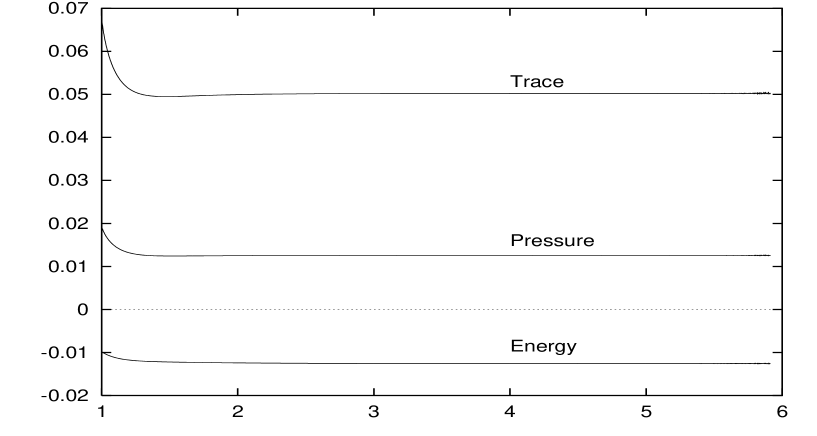
FIG. 9.: Renormalized value of $\langle\Phi^{2}\rangle_{R}$ as a function of comoving time for $m=0$, $\xi=0$, and $t_{0}=1.0$.

FIG. 10.: Energy, trace, and pressure as functions of comoving time for $m=0$, $\xi=0$, and $t_{0}=1.0$.

Notice that for the massless, minimally coupled case the late time behavior of the renormalized energy, trace, and pressure are determined by the value given in reference [22], and it does not go to the value calculated in reference [21]. This difference can be understood as a finite additional term that must be added to the Bunch-Davies result when the spatially homogeneous $k=1$ mode is handled properly.

It is interesting to study the case of the exactly massless, minimally coupled scalar field for a wider variety of initial conditions. If a non-zero number of particles $N_{k}$ in a finite number of modes is added, the asymptotic values of the renormalized $\langle T_{ab}\rangle$ still approaches the de Sitter invariant value [22]

$$\langle T_{ab}\rangle_{{}_{R}}\rightarrow{119\bar{H}^{4}\over 960\pi^{2}}g_{ab}\,,$$ (145)

even though the initial state and transient behavior in those cases (non-vacuum initial conditions) are not de Sitter invariant.

The fact that in all the above cases, even for de Sitter non-invariant initial conditions and even for the massless, minimally coupled field, the total renormalized energy-momentum tensor goes to the de Sitter form, $\varepsilon\rightarrow-p\rightarrow$ constant, is an important general conclusion of our study. Qualitatively, one can understand this result in the following way. At late times, $t\gg\bar{H}^{-1}$, $a(t)$ grows exponentially in de Sitter spacetime, and a very large number of modes have wavenumber $k\ll a$, i.e., physical wavelengths that have been redshifted out of the de Sitter horizon and frozen out. Those wavenumbers for which $k$ is still greater than $a(t)$ behave like adiabatic vacuum modes and are removed by the subtraction procedure. Hence the sums (integrals) over $k$ in the renormalized energy-momentum tensor are cut off at $k_{\rm max}$ of order $a(t)$. Since the initial conditions differ from the de Sitter invariant vacuum data only for some finite set of wavenumbers $k\leq k_{0}$ (say), these small wavenumbers make a decreasingly small contribution to the mode sum, which is controlled by the wide band of wavenumbers for which $k_{0}\ll k<a(t)$. The summand (integrand) in this wide $k$ band appearing in the energy density, pressure or trace is a function only of physical wavenumber $k/a$ (since it is independent of the initial data). Examining the behavior of the mode functions for late times and expanding the integrand in $\varepsilon$ or $p$ in powers of physical momentum it is easy to see that

$${1\over a^{3}(t)}\sum_{k=k_{0}}^{a(t)}k^{2}\left({a(t)\over k}\right)^{n} \simeq a^{n-3}(t)\int_{k_{0}}^{a(t)}k^{2-n}{\mathrm{d}}k=1-\left({k_{0}\over a(t)}\right)^{3-n}\;\rightarrow 1\;,\qquad{\rm for}\qquad n<3\;.$$ (146)

Hence all terms in the summand which do not grow faster than $n=3$ for large $a(t)$ yield a constant contribution to $\langle T_{ab}\rangle$ in the late time limit, independent of the initial data. The largest power $n$ which can occur in the mode sums for $\varepsilon$ and $p$ is controlled by the behavior of the mode functions $f_{k}$ at late times. Referring back to Eqs. (29) and (30) it is clear that the late time behavior of $f_{k}(t)$ is oscillatory, $\exp(\pm i\gamma\bar{H}t)$ for $\gamma^{2}\geq 0$ but exponential, $\exp(\pm|\gamma|\bar{H}t)$ for $\gamma^{2}<0$. Since $\langle T_{ab}\rangle$ is bilinear in the mode functions the power $n$ can be as large as $2|\gamma|$ for $\gamma$ pure imaginary. Provided $\gamma^{2}>-{9\over 4}$, all $n<3$, and the exponential behavior cannot overcome the normal kinematic redshift $a^{-3}$, there are no extreme infrared singular terms in the summand, and we conclude from (146) that both $\varepsilon$ and $p$ should tend asymptotically to a constant, independent of the initial data at late times. By the covariant conservation equation (83) for the renormalized $\langle T_{ab}\rangle$ this implies the de Sitter equation of state $\varepsilon\rightarrow-p$ at late times, which is precisely what the numerical results show.

Conversely, if $\gamma^{2}<-{9\over 4}$, we should expect the integrals for the finite renormalized energy density and pressure of the scalar field to contain terms with $n=2|\gamma|>3$ and to grow with the scale factor like $a^{2|\gamma|-3}$ [7]. Details of this case and the analytic calculation of this behavior will be presented elsewhere [24].

The case $\gamma^{2}=-{9\over 4}$ is marginal. For this value of $\gamma^{2}$ the power $n=3$ is possible (but not required) in the mode sum. If present, it leads to a logarithm, $\log a\rightarrow\bar{H}t$ and linear growth in cosmic time for the components of the energy-momentum tensor. One has to examine the energy-momentum tensor in more detail to determine if such logarithmic behavior exists or not, as a general argument based on the asymptotics of the mode equation (29) will not suffice. In the adiabatic ‘vacuum’ and matter contributions separately we observe this linear growth for the massless, minimally coupled scalar. This behavior of the ‘vacuum’ component is easily understood from the asymptotic forms of the functions $W_{k}$ and $V_{k}$ in (125) in the massless, minimally coupled case, since they imply that

$$\varepsilon^{\cal N}_{k}\rightarrow\left({a\over k}\right)^{3}\,,$$ (147)

for $k\ll a$. This is the marginal $n=3$ power behavior which leads to a linear growth (for the energy density of the vacuum contribution) in comoving time with slope $(8\pi^{2})^{-1}$. However, it turns out that for the exactly massless, minimally coupled case ($m^{2}=\xi=0$) the complete, vacuum plus particle, renormalized energy and pressure do not have such $n=3$ logarithmic divergences, as our numerical studies show. In this case there is an exactly compensating growth in the matter contribution which cancels the vacuum piece. This cancellation is a consequence of the exact field translational symmetry ($\Phi\to\Phi+{\rm constant}$ ) in the massless, minimally coupled case which prevents a term proportional to $\langle\Phi^{2}\rangle$ from appearing in $\langle T_{ab}\rangle$.

Next we consider $\gamma^{2}=-{9\over 4}$, i.e., $m^{2}+12\xi\bar{H}^{2}=0$, with $m^{2}$ and $\xi$ separately different from zero, which has the same mode equation but no such symmetry under field translations. Because the energy-momentum tensor (77) depends on $m^{2}$ and $\xi$ in distinctly different ways, in these cases there is a generic term proportional to $\langle\Phi^{2}\rangle$ in $\varepsilon$ and $p$, and hence the exact cancellation of the linear growth in $t$ between vacuum and particle contributions no longer occurs. The total energy-momentum tensor now grows logarithmically with $a(t)$ or linearly with $t$ in de Sitter space. This behavior is illustrated in Fig. 11.

FIG. 11.: Energy, trace, and pressure as functions of comoving time for $m=0.3$, $\xi=-0.0075$, and $t_{0}=1.0$.

The coefficients of this linear growth can be determined analytically from the known behavior of $\langle\Phi^{2}\rangle$, namely

$$\varepsilon \rightarrow -{3\xi\bar{H}^{5}\over 4\pi^{2}}t+\varepsilon_{0}\,,$$ (148)

$$p \rightarrow +{3\xi\bar{H}^{5}\over 4\pi^{2}}t+p_{0}\,,$$ (149)

$$\langle T\rangle \rightarrow +{12\xi\bar{H}^{5}\over 4\pi^{2}}t+T_{0}\,,$$ (150)

with the constants $\varepsilon_{0}$ and $p_{0}$ constrained by the conservation equation (83) to obey

$$\varepsilon_{0}+p_{0}=\xi{\bar{H}^{4}\over 4\pi^{2}}\,,$$ (151)

and the constant $T_{0}$ determined by the equation

$$T_{0}=3p_{0}-\varepsilon_{0}\,.$$ (152)

Hence for $\xi>0$ (and $m^{2}<0$) this linear growth decreases the effective cosmological constant over time, whereas for $\xi<0$ (and $m^{2}>0$) it increases it. In either case the backreaction of the scalar quantum field cannot be neglected at late times. It remains to be seen whether this linearly growing behavior carries over to the physically more relevant case of one-loop metric fluctuations themselves, and if so with which sign.

Finally, it is interesting to study the case of minimal coupling and non-vanishing but small real mass. In this case there are two time scales: a short time scale on which the Allen-Folacci vacuum is approached, and a longer time scale controlled by $1/m$ on which there is a smooth transition to the Bunch-Davies vacuum. Details of this case and a reliable analytic calculation of the behavior observed will be presented elsewhere [24].

VI Conclusions

We have presented a general method to study the initial value problem of a quantum field in a FRW spacetime. The two basic ingredients are: an initial adiabatic state (of order four), and an adiabatic number basis, with respect to which we define a particle number. This basis allows one to write the bare energy-momentum tensor as a sum of two contributions: a vacuum polarization term, and a particle production term. The advantage of the basis presented here is that the non-universal power law divergences of $\langle T_{ab}\rangle$ are isolated in the vacuum polarization piece, and the matter contribution displays physically reasonable behavior, as evidenced by the particle creation process in de Sitter space. We have implemented a numerical scheme incorporating this theoretical approach which preserves the covariant conservation of $\langle T_{ab}\rangle$, and yields a renormalized $\langle T_{ab}\rangle$ which is cutoff independent.

The numerical results for a de Sitter background can be summarized as follows. For the case of large mass ($\gamma\geq 0$) particle production takes place at horizon crossing, and the late time behavior of the renormalized energy-momentum tensor agrees with that of the Bunch-Davies vacuum. In the conformally invariant case ($m=0,\xi=1/6$) there is no particle production, and the renormalized value of the energy-momentum tensor corresponds to the well-known trace anomaly. The massless minimally coupled field ($m=0,\xi=0$) appears to be a marginal case. Non-de Sitter invariant initial conditions are driven to the Allen-Folacci vacuum, and not to the Bunch-Davies vacuum. In none of the above cases does $\langle T_{ab}\rangle$ vanish for late times, that is, it is not red-shifted away due to the expansion of the universe. Backreaction effects, though not required by this behavior cannot be ruled out when higher order corrections due to self-interactions or fluctuations in the background metric are included. Finally, for $m^{2}+\xi R=0$, but $m^{2}$ and $\xi$ individually different from zero, the total energy density, trace, and pressure of a free scalar field grow without bound, logarithmically with the scale factor. In this case it is certain that backreaction effects must be included self-consistently, since the energy density and pressure must eventually grow large enough to influence the background geometry and invalidate the test field approximation.

We believe that these results merit a fuller investigation of the effects of self-interactions and quantized gravitational fluctuations in a complete backreaction calculation. With respect to the latter, an interesting extension of the present study of free scalar field theory would be to the second order energy-momentum tensor of quantized metric fluctuations themselves. Barring a special cancellation which occurs in the $\xi=m=0$ scalar case, we may expect that this energy-momentum tensor would contain terms which grow logarithmically with the scale factor, and dynamically influence the evolution of the mean geometry away from de Sitter space, as has been suggested by general arguments some time ago [35]. The generalization to fully self-interacting fields is another interesting direction to pursue, since one would again expect the interactions to alter the de Sitter equation of state found in our study of the asymptotic behavior of massive fields. The formalism presented in this paper is intended to serve as a foundation from which the detailed analyses of these issues can begin, and the general backreaction problem in cosmological spacetimes with arbitrary finite adiabatic initial data can be posed and solved numerically. These extensions, applications to specific cosmological models, and the generation of density perturbations in the early universe are under current study.

A Adiabatic Expansion in Conformal and Comoving Time

Because of the loss of explicit covariance under time reparameterizations in the adiabatic regularization procedure, we establish in this Appendix the relationship between the adiabatic expansions in two different, commonly used time coordinates, namely conformal time $\eta$ and the comoving time $t$ employed in the present work. We will show that the two adiabatic expansions (comoving and conformal) give identical results for physical quantities such as $\langle T_{ab}\rangle$ to any order in the expansion.

The relation between the two time coordinates is given by (3) of the text. We denote a derivative with respect to comoving time by a dot, and a derivative with respect to conformal time by a prime. If we define the conformal mode functions by the relation,

$$g_{k}(\eta)=a^{-{1\over 2}}(t)f_{k}(t)\;,$$ (A1)

then the mode equation (29) in comoving time implies the mode equation,

$$g^{\prime\prime}_{k}(\eta)+\varpi^{2}_{k}(\eta)g_{k}(\eta)=0\,,$$ (A2)

with

$$\varpi^{2}_{k}(\eta)=C(\eta)\omega_{k}^{2}+\left(\xi-\frac{1}{6}\right)C(\eta)R(\eta)=a^{2}\Omega_{k}^{2}+a^{2}\left({\dot{H}\over 2}+{H^{2}\over 4}\right)\,,$$ (A3)

in conformal time. Hence the zeroth order adiabatic frequency for the adiabatic expansion in conformal time is $a$ times the zeroth adiabatic frequency for the adiabatic expansion in comoving time, $\omega_{k}$. We will now show that this feature holds to any adiabatic order.

Since the mode equations, (A2) or (29), both have the standard form of a time dependent harmonic oscillator equation, the adiabatic ansatz,

$$g_{k}(\eta)\equiv{1\over{{[2\Upsilon_{k}(\eta)]}^{1/2}}}{\rm exp}\left[-i{\int^{\eta}{\mathrm{d}}\eta^{\prime}\Upsilon_{k}(\eta^{\prime})}\right]\,,$$ (A4)

leads to an equation for $\Upsilon_{k}(\eta)$ in conformal time,

$$\Upsilon^{2}_{k}=\varpi^{2}_{k}+{3\over 4}\frac{1}{\Upsilon_{k}^{2}}{\left(\frac{{\mathrm{d}}\Upsilon_{k}}{{\mathrm{d}}\eta}\right)}^{2}-{1\over 2}\frac{1}{\Upsilon_{k}}\frac{{\mathrm{d}}^{2}\Upsilon_{k}}{{\mathrm{d}}\eta^{2}}\,,$$ (A5)

which is exactly of the same form as that in comoving time, upon replacing $\Upsilon_{k}$ by $W_{k}$, and $\varpi_{k}$ by $\Omega_{k}$, i.e.,

$$W^{2}_{k}=\Omega^{2}_{k}+{3\over 4}\frac{1}{W_{k}^{2}}{\left(\frac{{\mathrm{d}}W_{k}}{{\mathrm{d}}t}\right)}^{2}-{1\over 2}\frac{1}{W_{k}}\frac{{\mathrm{d}}^{2}W_{k}}{{\mathrm{d}}t^{2}}\,.$$ (A6)

To zeroth adiabatic order we have established already that

$$\Upsilon_{k}^{(0)\,2}=CW_{k}^{(0)\,2}=C\omega_{k}^{2}\,.$$ (A7)

Let us now assume that this result is true at adiabatic order $N-1$, i.e.,

$$\Upsilon_{k}^{(N-1)2}(\eta)=C(t)W_{k}^{(N-1)2}(t)\,.$$ (A8)

and iterate to order $N$. Since

$$\frac{{\mathrm{d}}\Upsilon_{k}^{(N-1)}}{{\mathrm{d}}\eta} = a^{2}\left[HW^{(N-1)}_{k}+\dot{W}_{k}^{(N-1)}\right]\,,$$ (A9)

$$\frac{{\mathrm{d}}^{2}\Upsilon_{k}^{(N-1)}}{{\mathrm{d}}\eta^{2}} = a^{3}\left[2H^{2}W^{(N-1)}_{k}+\dot{H}W^{(N-1)}_{k}+3H\dot{W}_{k}^{(N-1)}+\ddot{W}_{k}^{(N-1)}\right]\,,$$ (A10)

substitution into the right side of (A5) and using (A3) gives the desired iteration to order $N$, namely,

$$\Upsilon^{(N)2}_{k} = \varpi^{2}_{k}+{3\over 4}\frac{1}{\Upsilon_{k}^{(N-1)2}}{\left(\frac{{\mathrm{d}}\Upsilon_{k}^{(N-1)}}{{\mathrm{d}}\eta}\right)}^{2}-{1\over 2}\frac{1}{\Upsilon_{k}^{(N-1)}}\frac{{\mathrm{d}}^{2}\Upsilon_{k}^{(N-1)}}{{\mathrm{d}}\eta^{2}}$$ (A11)

$$= a^{2}\left[\Omega_{k}^{2}+{3\over 4}\frac{1}{W_{k}^{(N-1)2}}{\left(\frac{{\mathrm{d}}W_{k}^{(N-1)}}{{\mathrm{d}}t}\right)}^{2}-{1\over 2}\frac{1}{W_{k}^{(N-1)}}\frac{{\mathrm{d}}^{2}W_{k}^{(N-1)}}{{\mathrm{d}}t^{2}}\right]$$ (A12)

$$= a^{2}W_{k}^{(N)2}\,.$$ (A13)

Hence by induction we have proven that to any adiabatic order

$$\Upsilon^{(N)}_{k}(\eta)=a(t)W_{k}^{(N)}(t)\,.$$ (A14)

Moreover it is clear that this argument has relied only on the form of the mode equation (29) or (A2), and their corresponding WKB definition of the frequencies $W_{k}$ and $\Upsilon_{k}$. Since under an arbitrary differentiable transformation of time coordinates,

$${\mathrm{d}}t=b(t^{\prime}){\mathrm{d}}t^{\prime}\;,$$ (A15)

the mode functions can be rescaled,

$$f_{k}(t)=b^{-{1\over 2}}(t^{\prime})g_{k}(t^{\prime})\;,$$ (A16)

in order for the first $t^{\prime}$ derivative terms in $\ddot{f}_{k}$ to be eliminated, the mode equation in the new time variable can be put in the standard form,

$$g^{\prime\prime}_{k}(t^{\prime})+\varpi^{2}_{k}(t^{\prime})g_{k}(t^{\prime}) = 0\;,\,\qquad{\rm with}\qquad\varpi^{2}_{k}(t^{\prime})=b^{2}\Omega_{k}^{2}-{3\over 4}\left({b^{\prime}\over b}\right)^{2}+{b^{\prime\prime}\over 2b}\,,$$ (A17)

where now the prime denotes differentiation with respect to $t^{\prime}$. Once in this form the adiabatic ansatz (A5) may be inserted and the previous inductive argument may be repeated to yield

$$\Upsilon^{(N)}_{k}(t^{\prime})=bW_{k}^{(N)}(t)\,.$$ (A18)

for the arbitrary reparameterization of the time coordinate, $t\rightarrow t^{\prime}(t)$.

An immediate corollary of this result is that any quantity such as the energy density and pressure, developed up to a given adiabatic order $N$ in the comoving time coordinate $t$ corresponds exactly to the same quantity developed up to the same adiabatic order $N$ in any other time coordinate $t^{\prime}$. Since $T_{ab}$ transforms as a tensor, the energy density and pressure transform as

$$\varepsilon \rightarrow \varepsilon^{\prime}=b^{2}\varepsilon\,,$$ (A19)

$$p \rightarrow p^{\prime}=p\;,$$ (A20)

under (A15). Hence up to the overall factor of $b^{2}$ in the first of these relations, the energy density and pressure in either time coordinate are numerically equal at any order of the adiabatic expansion, and the renormalization procedure of subtracting the expansion up to adiabatic order two or four from the bare quantities is the same procedure in any time coordinate. The case $t^{\prime}=\eta$ and $b=a$, relating conformal time to comoving time, is just a special case of this much more general result, so that the conformal adiabatic expansion which has been given, for example, in [14, 25] is exactly equivalent to the corresponding expansion in comoving time given by Eqns. (42) and (45) of the text, as may be checked by explicit comparison of the two sets of expressions. Hence the subtraction of the adiabatic order two expressions (107) from the bare energy density and pressure corresponds exactly to the same subtraction in conformal (or any other) time coordinate which leaves the spatial sections unchanged. Finally, since the fourth order logarithmic cutoff dependence of $\langle T_{ab}\rangle$ is proportional to the geometric tensor ${}^{(1)}H_{ab}$, this remaining cutoff dependence and the argument (given in the text) for how to handle it in backreaction calculations, applies equally well in any time coordinate.

REFERENCES

- [1] G.W. Gibbons, General Relativity: An Einstein Centenary Survey, edited by S.W. Hawking and W. Israel (Cambridge University Press, Cambridge, 1979) and references contained therein.
-
[2]
D.N. Page,
Phys. Rev. D 25, 1499 (1982).
M.R. Brown and A.C. Otewill, ibid. 31, 2514 (1985).
M.R. Brown, A.C. Otewill, and D.N. Page, ibid. 33, 2840 (1986).
V.P. Frolov and A.I. Zel’nikov, ibid. 35, 3031 (1987).
P.R. Anderson, W.A. Hiscock, and D.A. Samuel, Phys. Rev. Lett. 70, 1739 (1993).
P.R. Anderson, W.A. Hiscock, J. Whitesell, and J.W. York, Jr., Phys. Rev. D 50, 6427 (1994).
P.R. Anderson, W.A. Hiscock, and D.J. Loranz Phys. Rev. Lett. 74, 4365 (1995). -
[3]
T. Souradeep and V. Sahni,
Mod. Phys. Lett. A 7, 3541 (1992).
A.A. Starobinsky , JETP Lett. 30, 719 (1979).
L.F. Abbot and M.B. Wise, Nucl. Phys. B 135, 279 (1984).
B. Allen, Phys. Rev. D 37, 2078 (1988).
V. Sahni, ibid. 42, 453 (1990).
B.-L. Hu and L. Parker, Phys. Lett. A 63, 217 (1977). -
[4]
L.H. Ford,
Phys. Rev. D 35, 2955 (1987).
L. Kofman, A. Linde, and A.S. Starobinsky, ibid. 56, 3258 (1997), Phys. Rev. Lett. 73, 3195 (1994).
D. Boyanovsky, D. Cormier, H.J. de Vega, R. Holman, A. Singh, and M. Srednicki, hep-ph/9609527.
D. Boyanovsky, H.J. de Vega, R. Holman, D.-S. Lee, and A. Singh, Phys. Rev. D 52, 6805 (1995). -
[5]
B.-L. Hu and L. Parker,
Phys. Rev. D 17, 993 (1978).
J.B. Hartle and B.-L. Hu, ibid. 21, 2756 (1980). -
[6]
L. Parker,
gr-qc/9804002.
L. Parker and A. Raval, gr-qc/9905031.
P.J.E. Peebles and A. Vilenkin, astro-ph/9810509. - [7] V. Sahni and S. Habib, Phys. Rev. Lett. 81, 1766 (1998).
- [8] P.R. Anderson and C.D. Mull, Phys. Rev. D 59, 044007 (1999) and references contained therein.
-
[9]
Paul R. Anderson,
Phys. Rev. D 28, 271 (1983),
ibid. 29, 615 (1984),
ibid. 32, 1302 (1985),
ibid. 33, 1567 (1986).
Wai-Mo Suen, Phys. Rev. D 35, 1793 (1987), ibid. 40, 315 (1989), Phys. Rev. Lett. 62, 2217 (1989).
Wai-Mo Suen and Paul R. Anderson, Phys. Rev. D 35, 2940 (1987).
N.C. Tsamis and R.P. Woodard, Annals of Phys. 253, 1 (1997). -
[10]
B. S. DeWitt,
Phys. Rep. 19C, 295 (1975).
T. S. Bunch, J. Phys. A: Math. Gen. 11, 603 (1978), ibid. 12, 517 (1979).
T. S. Bunch, S. M. Christensen, and S. A. Fulling, Phys. Rev. D 18, 4435 (1978).
T. S. Bunch and P. C. W. Davies, J. Phys. A: Math. Gen. 11, 1315 (1978), Proc. R. Soc. Lond. A 356, 569 (1977), ibid. 357, 381 (1977).
P.C.W. Davies, S.A. Fulling, S.M. Christensen, and T.S. Bunch, Annals Phys. 109, 108 (1977). -
[11]
N. D. Birrell and P. C. W. Davies,
Quantum fields in curved space,
(Cambridge University Press, England, 1982)
and references contained
therein.
S. A. Fulling, Aspects of quantum field theory in curved space-time, (Cambridge University Press, England, 1989).
A. A. Grib, S. G. Mamayev and V. M. Mostepanenko, Vacuum quantum effects in strong fields, (Friedmann Laboratory Publishing, St. Petersburg, 1994) and references contained therein. -
[12]
S. A. Fulling and L. Parker,
Ann. Phys., NY 87, 176 (1974).
L. Parker and S. A. Fulling, Phys. Rev. D 9, 341 (1974).
T. S. Bunch, J. Phys. A: Math. Gen. 13, 1297 (1980). - [13] N. D. Birrell, Proc. R. Soc. B 361, 513 (1978).
- [14] Paul R. Anderson and Leonard Parker, Phys. Rev. D 36, 2963 (1987).
- [15] S. M. Christensen, Phys. Rev. D 14, 2490 (1976), ibid. 17, 946 (1978).
- [16] S. Habib, Y. Kluger, E. Mottola, and J.P. Paz, Phys. Rev. Lett. 76, 4660 (1996).
- [17] F. Cooper, S. Habib, Y. Kluger, and E. Mottola, Phys. Rev. D 55, 6471 (1997).
- [18] Y. Kluger, E. Mottola, and J. Eisenberg, Phys. Rev. D 58, 125015 (1998).
-
[19]
F. Cooper and E. Mottola,
Phys. Rev. D 36, 3114 (1987).
J. Lindig, ibid. 59, 064011 (1999). -
[20]
D. Boyanovsky, D. Cormier, H.J. de Vega, and R. Holman,
Phys. Rev. D 55, 3373 (1997).
D. Boyanovsky, D. Cormier, H.J. de Vega, R. Holman, A. Singh, and M. Srednicki, ibid. 56, 1939 (1997). - [21] T.S. Bunch and P.W. Davies, Proc. R. Soc. Lond. A 360, 117 (1978).
-
[22]
B. Allen and A. Folacci,
Phys. Rev. D 35, 3771 (1987).
K. Kirsten and J. Garriga, ibid. 48, 567 (1993). - [23] I. Antoniadis and E. Mottola, Phys. Rev. D 45, 2013 (1992).
- [24] P. Anderson, S. Habib, C. Molina-París, and Emil Mottola, (in preparation).
- [25] T. S. Bunch, J. Phys. A: Math. Gen. 13, 1297 (1980).
- [26] L. Parker, Phys. Rev. 1057 (1969), Phys. Rev. D 3, 346 (1971).
-
[27]
Ya.B. Zel’dovich and A.A. Starobinsky,
Sov. Phys. (JETP) 34, 1159 (1972).
B.-L. Hu and L. Parker, Phys. Rev. D 17, 993 (1978), Phys. Lett. A 63, 217 (1977). - [28] S. A. Fulling, L. Parker, and B. L. Hu, Phys. Rev. D 10, 3905 (1974).
- [29] F. Cooper, S. Habib, Y. Kluger, E. Mottola, J.P. Paz, and P. Anderson, Phys. Rev. D 50, 2848 (1994).
- [30] Leonard Parker and Jonathan Z. Simon, Phys. Rev. D 47, 1339 (1993).
- [31] B. Allen, Phys. Rev. D 32, 3163 (1985).
- [32] A. A. Starobinsky, in Fundamental Interactions (MGPI Press, Moscow, 1983); in Current Topics in Field Theory, Quantum Gravity, and Strings edited by H. J. deVega and N. Sánchez (Springer, New York, 1986). See also, A. Vilenkin, Nuc. Phys. B 226, 527 (1983).
- [33] S. Habib, Phys. Rev. D 46, 2408 (1992) and references contained therein.
- [34] E. Mottola, Phys. Rev. D 31, 754 (1985).
- [35] E. Mottola, Talk contributed at the workshop on “Physical Origins of Time Asymmetry”, Mazagón (Huelva), Spain, (Cambrigde University Press, 1991).