A Numerical Study of Boson Stars:
Einstein Equations with a
Matter Source

WASHINGTON UNIVERSITY
Department of Physics

A NUMERICAL STUDY OF BOSON STARS:
EINSTEIN EQUATIONS WITH A
MATTER SOURCE

a dissertation presented to the
graduate school of arts and sciences
of washington university in
partial fulfillment of the
requirements for the degree
of doctor of philosophy

© Copyright 2024
by
Jayashree Balakrishna

I certify that I have read this thesis and that in my opinion it is fully adequate, in scope and in quality, as a dissertation for the degree of Doctor of Philosophy.

  Wai-Mo Suen/Matt Visser (Principal Advisor)

I certify that I have read this thesis and that in my opinion it is fully adequate, in scope and in quality, as a dissertation for the degree of Doctor of Philosophy.

  Clifford M. Will

I certify that I have read this thesis and that in my opinion it is fully adequate, in scope and in quality, as a dissertation for the degree of Doctor of Philosophy.

  Carl M. Bender

Approved for the University Committee on Graduate Studies:

  Dean of Graduate Studies & Research

Abstract

The study of the properties and dynamics of self-gravitating bosonic objects in Einstein gravity was conducted. Bosons are promising candidates for dark matter. They can form compact objects through a Jeans instability mechanism. We studied boson stars made up of self-gravitating scalar fields, with and without nonlinear self-couplings. These are non-topological solutions of the coupled Einstein–Klein–Gordon equations. We studied the stability of boson stars in the ground and excited states, and determined the quasinormal mode ($QNM$) frequencies of stable boson stars in spherical symmetry. The study was carried out in the standard Einstein theory of General Relativity and in Brans–Dicke theory. We also studied the formation of these objects in Brans–Dicke theory showing that they can form from the self-gravitation of bosonic matter. We also studied the possibility of a bosonic halo surrounding galaxies. These halo models predict the observed flatness of galactic curves. We studied their formation and stability.

After an extensive study in spherical symmetry we carried out numerical studies of boson star dynamics in full 3+1 dimension. One focus of the 3 spatial dimension (3D) study was on the validation of the numerical code constructed to solve Einstein equations with matter sources. The use of the scalar field has unique advantages: Boson Stars do not suffer from difficulties associated with hydrodynamic sources (like shock waves or the surface problems of neutron stars). They also do not suffer from the difficulties related to the singularities of black holes. The code was first tested with spherical perturbations and compared with the spherical results. We determined the coordinate conditions needed to provide stable evolutions under radial perturbations. We then went on to study their behavior under non-spherical perturbations. Both scalar and gravitational radiation produced under these perturbations were studied. We reproduced the $QNM$ frequencies of the stars, as determined by perturbation studies carried out by other groups. The energy generated by the perturbation was studied with different radiation indicators. We also observed the collapse to black holes of unstable boson-star configurations. We simulated the collision of two boson stars. This is of interest as the two body problem is as yet unresolved in general relativity.

Chapter 1 Introduction

The study of bosonic compact objects is motivated by several considerations. From a purely aesthetic point of view, the existence of compact objects made up of fermionic subparts (like neutron stars), leads one to postulate the existence of bosonic counterparts made up of particles satisfying Bose-Einstein statistics. This was the motivation for the original works of Kaup  [1], and Ruffini and Bonazzola [2].

Although not observed thus far, these purely theoretical objects nevertheless can provide many useful physical insights. They can be a source of scalar radiation and gravitational radiation, and can under certain conditions collapse to black holes. Studying the evolution of the resultant black holes then adds a new dimension to black hole studies since now matter is present in the spacetime.

Recently, Bosonic objects have been suggested as strong candidates for dark-matter in the universe. This has changed their status from being purely theoretical toy models, to possibly being extremely real physical objects.

They also occupy a significant place in the field of numerical relativity. For the first time one can consider the full Einstein system of equations with matter sources present. Before the advent of this field, boson stars could only be studied under infinitesimal perturbations using perturbative techniques [3, 4].

In one-dimensional numerical relativity we have observed the behavior of boson stars under larger and more general spherical perturbations. In $3D$, for the first time, a fully relativistic problem with matter present was considered. Boson stars provide a model which does not suffer from the problematic singularities of black-hole spacetimes. In addition the presence of a scalar field with an exponential fall-off that, in principle, stretches to spatial infinity, prevents the formation of sharp outer surfaces that are characteristic of neutron stars.

The $3D$ code could be tested against the well studied 1D codes by considering spherical perturbations. The gravitational wave signals of non-spherical configurations in the linear regime were compared against the results of linear non-spherical perturbation studies. A comparison of the signals calculated by different methods provided a further successful code test. In order to stabilize the code, various numerical techniques were implemented and studied. With a stable code one could then study the signals that came out of large non-spherical perturbations. These physical studies were precursors to a planned series of future neutron star studies. The collapse of an unstable boson star to a black hole, followed by a “turning on” of apparent horizon boundary conditions, was a new aspect of black hole studies that boson stars provided. In addition we began simulations of the collision of two boson stars. This is of importance in the generalized two-body problem since the resulting dynamics may not be sensitively dependent on the constituent objects.

A study of compact bosonic objects touched upon numerous physical issues. In one dimension, the evolution of boson stars in the ground and excited states, with and without self-coupling, and the evolution and formation of boson-stars in Brans-Dicke theory were investigated. The stability and formation of objects formed from massless scalar fields was also studied in a one-dimensional halo model. In 3D the study of gravitational waves from the non-spherical perturbation of a boson star was followed by a study of black hole evolutions of the black holes formed from collapsed boson stars.

We begin by introducing the Einstein equations with general matter sources, followed by a historical perspective on the nature of boson stars and a summary of earlier work in the field. The notion of dark matter is then introduced, what makes one believe it exists, and why bosons are good candidates for it. This is followed by the basics of a Jeans instability mechanism to give an idea of how boson stars could actually form.

The final topics in the introduction are about boson stars without spherical symmetry. Since they can be a source of gravitational waves, we first review how Einstein’s equations predict gravitational radiation in a non-spherically symmetric setting. In this regard we also introduce the idea of waveform extraction through the Zerilli, Bel-Robinson, and Newman-Penrose functions which we use in our code. We discuss some of the other work in the field of Boson stars in higher dimensions as well as the results of $3D$ perturbation studies to which we compare our results. The penultimate topic in the introduction is about the $3+1$ $ADM$ split of space-time and how the Einstein equations can be separated into constraint and evolution equations. Since our work is numerical, we also present an overview of the kinds of difficulties that we face in a general numerical code. The actual details of the code and numerics are explained in the chapters that follow.

1.1 Einstein Equations with Matter: Variational Approach

The central tenet of GR is that matter must respond to geometry by moving in a certain way, and geometry must in turn respond to matter by curving. We briefly outline the various quantities that we encounter in the equations that we will have to solve, and then use a variational approach to derive the equations which a fully relativistic system with matter sources must obey [5].

• Metric: The invariant measure of proper length or proper time between neighboring events in spacetime is given by

  $$ds^{2}=g_{\mu\nu}\;dx^{\mu}\;dx^{\nu}=-d\tau^{2},$$ (1)

  where the metric $g_{\mu\nu}$ in a Minkowski spacetime is the diagonal metric $\eta_{ij}=diag(-1,1,1,1)$.

• $\Gamma$: In curved space variations in tensors are affected by the fact that the basis vectors themselves are twisting and turning from spacetime point to spacetime point. The Connection Coefficient $\Gamma$ measures the changes in the basis vectors through the relation

  $${\bf\nabla}_{\nu}{\bf e}_{\mu}=\Gamma^{\delta}{}_{\mu\nu}\;{\bf e}_{\delta}.$$ (2)

  Here ${\bf\nabla}_{\nu}$ measures changes along the basis vector ${\bf e}_{\nu}$. In any coordinate basis ($[{\bf e}_{\mu},{\bf e}_{\nu}]=0$ ) the connection coefficients are given by

  $$\Gamma^{\alpha}{}_{\mu\nu}=\frac{1}{2}\,g^{\alpha\delta}\left(g_{\delta\mu,\nu}+g_{\delta\nu,\mu}-g_{\mu\nu,\delta}\right)=\Gamma^{\alpha}{}_{\nu\mu}.$$ (3)

• Geodesic Equation: The path of particles between spacetime points ${\cal P}$ and ${\cal Q}$ is one that extremizes $\int_{\cal P}^{\cal Q}\,d\tau$ leading to the geodesic equation

  $$\frac{d^{2}x^{\beta}}{{d\lambda}^{2}}+\Gamma^{\beta}{}_{\mu\nu}\frac{dx^{\mu}}{d\lambda}\frac{dx^{\nu}}{d\lambda}=0,$$ (4)

  where $\lambda$ is a parameter that parametrizes the path and agrees with the proper time $\tau$ within $\lambda=a\tau+b$, with arbitrary constants $a$ and $b$.

• Riemann tensor: Spacetime curvature results in geodesics deviating from nearby geodesics, with test particles accelerating relative to one another. Measuring the deviation of one geodesic from another involves quantifying this curvature through the Riemann curvature tensor. In flat space (zero curvature) it must vanish. The Riemann curvature tensor components in terms of the connection coefficients are

  $$R^{\lambda}{}_{\alpha\mu\beta}=\frac{\partial\Gamma^{\lambda}{}_{\alpha\beta}}{\partial x^{\mu}}-\frac{\partial\Gamma^{\lambda}{}_{\alpha\mu}}{\partial x^{\beta}}+\Gamma^{\lambda}{}_{\sigma\mu}\Gamma^{\sigma}{}_{\alpha\beta}-\Gamma^{\lambda}{}_{\sigma\beta}\Gamma^{\sigma}{}_{\alpha\mu}.$$ (5)

  Physically in a curved spacetime parallel transport of a vector around a closed loop brings it back to the original point visibly changed. The Riemann tensor is a measure of the change. A 4 vector $A$ transported around a closed curve formed by vectors ${\bf u}$ and ${\bf v}$ (and their commutator to close the gap) suffers a change

  $$\delta A^{\alpha}+R^{\alpha}{}_{\beta\gamma\delta}\;A^{\beta}\;u^{\gamma}\;v^{\delta}=0.$$ (6)

  The Ricci tensor and scalar follow from $R_{\mu\nu}=R^{\alpha}{}_{\mu\alpha\nu}$ and $R=g^{\mu\nu}R_{\mu\nu}$.

In contrast to the geometrical quantities above, the stress energy tensor ${\bf T}$ contains information about the matter sources of gravity. The conditions of energy and momentum conservation are contained in the relation ${\bf\nabla\cdot T}=0$. The components of $T_{\mu\nu}$ are symmetric.

The equations that we must rely on to tell us how the system behaves are the Einstein equations

$${\bf G}=8\,\pi\,{\bf T},$$ (7)

where the geometry of spacetime that tells matter how to move is on the left hand while the matter sources telling spacetime how to curve are on the right hand. Thus ${\bf G}$ must only be geometry dependent and so must be entirely made from the Riemann tensor and the metric. For simplicity it is made linear in the Riemann tensor and since it is an indication of curvature it must vanish in flat space. Like the right hand side, it must be a dual tensor that is symmetric. The only second rank tensor we can build fulfilling these criteria is (up to an overall constant)

$$G_{\mu\nu}=R_{\mu\nu}-\frac{1}{2}R\;g_{\mu\nu}.$$ (8)

The factor $8\,\pi$ in (7) follows from comparisons to well known situations in Newtonian gravity ($g_{\mu\nu}\sim\eta_{\mu\nu}$).

It can be shown that we can associate the $tt$ component of the stress-energy tensor $T^{00}$ with the density of mass energy, while $T^{j0}$ is the density of the $j$ component of the momentum. The $00$ component of the Einstein equation is, therefore, called the Hamiltonian constraint and the $0i$ components are the momentum constraints.

The Einstein curvature tensor ${\bf G}$ has to have zero divergence and from this the divergence of $T_{\mu\nu}$ follows. Why this is so can be seen from the fact that a given spacetime hypersurface has a metric given by

$$ds^{2}=g_{\mu\nu}\;dx^{\mu}\;dx^{\nu}.$$ (9)

Using the metric symmetries we get ten independent components of $g_{\mu\nu}$. When the geometry evolves then, if we had ten independent equations

$$G_{\mu\nu}=8\,\pi\,T_{\mu\nu},$$ (10)

we could determine all ten $g_{\mu\nu}$ on a slice. This is not possible since we have the freedom to choose our coordinates:

$$x^{\mu}\rightarrow x^{{}^{\prime}\mu},$$ (11)

and this transformation would keep the line element (9) unchanged, but lead to the transformation $g_{\mu\nu}\rightarrow{g^{\prime}}_{\mu\nu}$. Therefore four of the ten conditions must be eliminated so that we have only six independent Einstein equations. Here is where the vanishing divergence of the geometry independent $T_{\mu\nu}$ plays a part. The equation

$$T^{\mu\nu}{}_{;\nu}=0,$$ (12)

gives us the required four conditions that are subtracted from the ten equations leaving six independent geometrical equations.

In order to actually derive equation (10), a variational principle is applied with action written in the form

$$I=\int\,{\cal{L}}\;d^{4}x=\int\,L\,(-g)^{\frac{1}{2}}\;d^{4}x.$$ (13)

The Lagrangian density is separated into a geometrical and a field part

$${\cal{L}}={\cal{L}}_{\mathrm{g}eom}+{\cal{L}}_{\mathrm{f}ield}=(-g)^{\frac{1}{2}}\,L,$$ (14)

$$L=L_{\mathrm{g}eom}+L_{\mathrm{f}ield}.$$ (15)

One then extremizes this action. In the $ADM$ formalism, one finds it convenient to think of the dynamics as representing the evolution from the specified 3-geometries of an initial spacelike to a final spacelike slice. The action integral is to be extremized with regard to choice of spacetime between these faces:

$$S\equiv S({}^{3}\xi),$$ (16)

with the action changing with 3-geometry according to

$$\delta S=\int\,\pi^{ij}\;\delta g_{ij}\;d^{3}x.$$ (17)

Here $\pi^{ij}=\frac{\delta S}{\delta g_{ij}}$ is the field momentum conjugate to $g_{ij}$. Consider the simplest action principle one can imagine:

$$L_{geom}=\left(\frac{1}{16\pi}\right)\;{}^{4}\!R.$$ (18)

Here ${}^{4}\!R$ is the four-dimensional scalar invariant. To be an invariant, $L_{geom}$ must be independent of the choice of coordinate systems. In the neighborhood of a point one can always choose coordinates such that the first derivatives of $g_{\mu\nu}$ vanish. Therefore, apart from a constant, no scalar invariants can be built homogeneously out of the metric coefficients and their first derivatives. Unlike the case of mechanics one must, therefore, consider second derivatives of the metric coefficients. One then has 20 distinct components of the curvature tensor with six parameters of a local Lorentz transformation giving 14 distinct choices. Only, one of these, ${}^{4}\!R$, is linear in second derivatives of metric components.

$${}^{4}\!R=g^{\alpha\beta}\,R_{\alpha\beta},$$ (19)

where

$$R_{\alpha\beta}=R^{\lambda}{}_{\alpha\lambda\beta}.$$ (20)

Every $\Gamma$ should be symmetric in its two lower indices giving a total of $4\times(3*2+4)=40$ independent components. In order for the action to be an extremum, variations due to changes in $g^{\mu\nu}$, as well as the $\Gamma$s’ should vanish.

$$0=\delta I=\frac{1}{16\pi}\int\,\delta\left(g^{\alpha\beta}\,R_{\alpha\beta}\,\sqrt{-g}\right)\;d^{4}x+\int\,\delta\left[L_{\mathrm{f}ield}\,\sqrt{-g}\right]\;d^{4}x.$$ (21)

The $\Gamma$s themselves do not transform like tensors although their variations $\delta\Gamma$ do.

$$\Gamma^{\bar{\gamma}}{}_{{\bar{\alpha}}{\bar{\beta}}}=\left[\Gamma^{\lambda}{}_{\sigma\tau}\;\frac{\partial x^{\sigma}}{\partial x^{\bar{\alpha}}}\;\frac{\partial x^{\tau}}{\partial x^{\bar{\beta}}}+\frac{\partial^{2}x^{\lambda}}{\partial x^{\bar{\alpha}}\partial x^{\bar{\beta}}}\right]\frac{\partial x^{\bar{\gamma}}}{\partial x^{\lambda}}.$$ (22)

The last term destroys the tensor character of the $\Gamma$s but cancels in $\delta\Gamma^{\lambda}_{\sigma\,\tau}$. From the fact that tensors can be studied in any coordinate system, we conveniently choose one in which the $\Gamma$s vanish at the point in question and so from (5) (after replacing commas by semicolons for correct formulas in any coordinate system)

$$\delta R^{\lambda}{}_{\alpha\mu\beta}=\delta\Gamma^{\lambda}{}_{\alpha\beta;\mu}-\delta\Gamma^{\lambda}{}_{\alpha\mu;\beta},$$ (23)

and

$$\delta R_{\alpha\beta}=\delta\Gamma^{\lambda}{}_{\alpha\beta;\lambda}-\delta\Gamma^{\lambda}{}_{\alpha\lambda;\beta}.$$ (24)

Also

$$\delta(-g)^{\frac{1}{2}}=\frac{1}{2}\,(-g)^{-\frac{1}{2}}\;(-g)\;\frac{\delta g_{\mu\nu}}{g_{\mu\nu}}=-\frac{1}{2}\,(-g)^{\frac{1}{2}}\;g_{\mu\nu}\;\delta g^{\mu\nu}.$$ (25)

Thus from (21) we see that

$$\frac{1}{16\,\pi} \int\Bigg{\{}g^{\alpha\beta}\,R_{\alpha\beta}\left(-\frac{1}{2}\,\sqrt{-g}\,g_{\mu\nu}\,\delta g^{\mu\nu}\right)+g^{\alpha\beta}\,\delta R_{\alpha\beta}\,\sqrt{-g}$$ (26)

$$+ R_{\alpha\beta}\,\sqrt{-g}\,\delta g^{\alpha\beta}\Bigg{\}}\,d^{4}x+\int\,\delta\left(L_{\mathrm{f}ield}\,\sqrt{-g}\right)\;d^{4}x,$$ (27)

$$= \frac{1}{16\,\pi}\,\left[\int\,\left(-\frac{1}{2}\,g_{\alpha\beta}\,R+R_{\alpha\beta}+\left(\delta\Gamma^{\lambda}{}_{\alpha\beta;\lambda}-\delta\Gamma^{\lambda}{}_{\alpha\lambda;\beta}\right)\right)\sqrt{-g}\;\delta g^{\alpha\beta}\;d^{4}x\right]$$ (29)

$$\qquad+\int\,\delta\left(L_{field}\,\sqrt{-g}\right)\;d^{4}x.$$

The $\delta\Gamma$ term is evaluated as follows:

$$\frac{1}{16\pi}\,\int g^{\alpha\beta}\,\left(\delta\Gamma^{\lambda}{}_{\alpha\beta;\lambda}-\delta\Gamma^{\lambda}{}_{\alpha\lambda;\beta}\right)\,\sqrt{-g}\;d^{4}x$$ (30)

$$= \frac{1}{16\,\pi}\,\int\,\Bigg{(}+\left\{{g}^{\alpha\beta}\,\delta\Gamma^{\lambda}{}_{\alpha\beta}\right\}_{;\lambda}\,-{g}^{\alpha\beta}{}_{;\lambda}\,\delta\Gamma^{\lambda}{}_{\alpha\beta}$$ (31)

$$- \left\{{g}^{\alpha\beta}\,\delta\Gamma^{\lambda}{}_{\alpha\lambda}\right\}_{;\beta}+{g}^{\alpha\beta}{}_{;\beta}\,\delta\Gamma^{\lambda}{}_{\alpha\lambda}\Bigg{)}\,\sqrt{-g}\;d^{4}x.$$ (32)

Using the fact that the metric is covariantly constant ($g^{\alpha\beta}{}_{;\alpha}=0$) we get

$$\frac{1}{16\,\pi} \int\,g^{\alpha\beta}\,\left(\delta\Gamma^{\lambda}{}_{\alpha\beta;\lambda}-\delta\Gamma^{\lambda}{}_{\alpha\lambda;\beta}\right)\,\sqrt{-g}\;d^{4}x$$ (33)

$$= \frac{1}{16\,\pi}\,\int\,\left(\left\{{g}^{\alpha\beta}\,\delta\Gamma^{\lambda}{}_{\alpha\beta}\right\}_{;\lambda}\,-\left\{{g}^{\alpha\beta}\,\delta\Gamma^{\lambda}{}_{\alpha\lambda}\right\}_{;\beta}\right)\,\sqrt{-g}\;d^{4}x.$$ (34)

Using Gauss’ theorem we get an integral over the surface. Since variations vanish on the boundary this integral identically vanishes leaving

$$\frac{1}{16\,\pi}\,\left[\int\,\left(-\frac{1}{2}g_{\alpha\beta}\,R+R_{\alpha\beta}\right)\,\sqrt{-g}\,\delta g^{\alpha\beta}\;d^{4}x\right]+\int\,\delta\left(L_{\mathrm{f}ield}\,\sqrt{-g}\right)\;d^{4}x=0.$$ (35)

The stress-energy tensor is defined to be

$$T_{\alpha\beta}\equiv\frac{2}{(-g)^{\frac{1}{2}}}\,\left(\frac{{\delta{\cal L}_{\mathrm{f}ield}}}{\delta g^{\alpha\beta}}\right)=-\frac{2}{(-g)^{\frac{1}{2}}}\,\left(\frac{{\delta{\sqrt{-g}\,L_{\mathrm{f}ield}}}}{\delta g^{\alpha\beta}}\right).$$ (36)

Using this definition

$$\int\,\delta\left(L_{\mathrm{f}ield}\,\sqrt{-g}\right)\;d^{4}x=\int\,\delta g^{\alpha\beta}\frac{{\delta({\sqrt{-g}\,L_{\mathrm{f}ield}})}}{\delta g^{\alpha\beta}}\;d^{4}x=-\frac{1}{2}\,\int\,T_{\alpha\beta}\,\sqrt{-g}\,\delta g^{\alpha\beta}\;d^{4}x,$$ (37)

which gives the equations of motion

$$G_{\alpha\beta}=8\,\pi\,T_{\alpha\beta}.$$ (38)

If we now restrict attention to a matter Lagrangian that depends on the metric but not metric derivatives (this assumption holds for usual matter fields such as spinors, gauge bosons and minimally coupled scalars but fails for non-minimally coupled scalars), then

$$G_{\alpha\beta}=8\,\pi\left(g_{\alpha\beta}\,L_{\mathrm{f}ield}-2\,\frac{\partial L_{\mathrm{f}ield}}{\partial g^{\alpha\beta}}\right).$$ (39)

This then sets up the equations for general metrics and matter sources in GR. We then specialize them to particular metrics, for example, spherically symmetric spacetimes, and a particular matter source that describes bosonic spin zero objects. Since most of the work has been on boson stars we start by describing what those are.

1.2 What are Boson Stars?

Boson stars are compact self-gravitating objects made up of scalars that are held together by the balance between the attractive force of gravity and the dispersive effects of a wave equation. The scalar field is complex and satisfies the Klein–Gordon equation, and the system has field solutions with different numbers of nodes. The lowest energy state, or ground state, is characterized by a field distribution that has no nodes. Unlike the case of fermions, where one can invoke the perfect fluid approximation and write an equation of state, a system of bosons has an anisotropic distribution of stress near its center, making such a concept inadmissible. Nevertheless, they have many similar properties to neutron stars. For a review, see [6].

1.2.1 An Historical Perspective

From an historical point of view the study of boson stars began with the work of Kaup [1]. Electromagnetic geons, as introduced by Wheeler [7] were gravitational-electromagnetic objects satisfying the electromagnetic and gravitational field equations. Their spherical configurations were found to be in unstable equilibrium. Compelled by this concept, Kaup introduced a Klein–Gordon geon, which satisfied the coupled KG and Einstein equations (the KGE equations) in a spherically symmetric metric. From the Lagrangian

$$L=R+g^{\mu\nu}\;\phi^{\ast}{}_{;\mu}\,\phi_{;\nu}-\frac{m^{2}}{\hbar^{2}}\,\phi^{\ast}\,\phi,$$ (40)

with scalar field $\phi$ and a spherically symmetric metric

$$d\tau^{2}=b^{2}dt^{2}-r^{2}d\Omega^{2}-a^{2}dr^{2},$$ (41)

is derived a scalar field equation (in appropriately defined units)

$$\Psi^{\prime\prime}+\left(\frac{2}{r}+\nu^{\prime}-\lambda^{\prime}\right)\Psi^{\prime}+a^{2}\left(\frac{E^{2}}{b^{2}}-1\right)\Psi=0,$$ (42)

where $\phi(r,t)=e^{i\,E\,t}\Psi(r)$, $a=e^{\lambda}$ and $b=e^{\nu}$.

Transforming to a new radial coordinate $s$ where

$$s=\int_{0}^{r}\,\frac{a}{b}\;dr,$$ (43)

so that $ds/dr=a/b$, we get

$$\frac{d^{2}\Psi}{{ds}^{2}}+\frac{2}{r}\frac{b}{a}\frac{d\Psi}{ds}+\left(E^{2}-b^{2}\right)\Psi=0.$$ (44)

This equation is similar to the radial Schr$\ddot{\mathchoice{\hbox{{o}}}{\hbox{{o}}}{\hbox{{o}}}{\hbox{{o}}}}$dinger equation for a potential $b^{2}$. In the asymptotic region $b^{2}\sim 1-2\,M/r$ so the potential is similar to the hydrogen atom case in that it has a $1/r$ dependence. This suggests countably infinite localized solutions for $\Psi$ with different numbers of nodes. The conserved current associated with the $U(1)$ symmetry of the problem is

$$J_{\nu}=\frac{1}{2}\,i\,(\Phi^{\ast}{}_{;\nu}\,\Phi-\Phi_{;\nu}\,\Phi^{\ast}),$$ (45)

With the particle number times $m$ the mass of a single boson

$$N\,m=-i\int\,\sqrt{-g}\;J_{0}=\int\,r^{2}\,a\,b\,J^{4}\;dr.$$ (46)

The ground state solutions are then numerically obtained and a plot of mass and particle number profiles for different central densities is made. The nature of the plot is shown in Fig. 2 (chapter 2). The mass of the bosonic geon increases to a maximum and then starts to decrease as does the particle number with its maximum at the same value of central density. However $Nm$ is greater than the mass of the bosonic geon for central densities up to a point beyond the maximum.

This result is very interesting since the mass profile as a function of central field density is very similar to that of neutron stars and white dwarfs when plotted as a function of density $\rho$. This is so, as pointed out in this paper, despite the absence of an equation of state in the case of a the KGE system where the radial pressure $-T^{r}_{r}$ is different from $-T^{\theta}_{\theta}=-T^{\phi}_{\phi}$. Not only are the profiles similar, but remarkably, so also are the stability properties, although the usual perfect fluid approach to stellar stability can no longer be applied.

A first-order perturbation approach in spherical symmetry is developed in Kaup’s paper, whose essential features are that the metric components are perturbed as $\nu\rightarrow\nu+\delta\nu$ and $\lambda\rightarrow\lambda+\delta\lambda$ so that $\delta g_{rr}=-2\,a^{2}\delta\lambda$ where $\delta\nu$ and $\delta\lambda$ are functions of $r$ and $t$. The scalar field perturbation is of the form

$$\delta\Phi=e^{i\,E\,t}\,\left[R(r,t)+i\,I(r,t)\right].$$ (47)

All time dependences of the perturbations are taken to be of the form $e^{i\omega t}$ and solutions with imaginary $\omega$ or negative $\omega^{2}$ are obviously unstable. A variational approach follows, to establish the ground state $\omega$ and this gives an erroneous result that all ground state solutions are stable.

A Newtonian approach to the problem is presented in [2]. The nonrelativistic Schr$\ddot{\mathchoice{\hbox{{o}}}{\hbox{{o}}}{\hbox{{o}}}{\hbox{{o}}}}$dinger equation with a potential $V$ satisfying the Poisson equation $\nabla^{2}V=-4\pi G\rho$ is used. A mass profile plot as a function of central density yields a maximum mass of $1.653\,{M_{Pl}^{2}}/{m}$, far greater than the relativistic value of $0.633\,{M_{Pl}^{2}}/{m}$ because of the continued use of the Newtonian approach to dense configurations no longer in the Newtonian regime. In [8] an $N$-body Hamiltonian for an $N$ boson configuration interacting via Newtonian gravity is written. The hydrogen-like resulting Hamiltonian then yields a ground state expectation value by analogy. A lower bound on the ground state energy (better by a factor of almost 3 than that of [2]) is obtained by separating out the center of mass kinetic energy (which corresponds to the global motion of the system and should not contribute to the ground state energy). This is now much lower than the relativistic result. A semi-relativistic calculation with a Hamiltonian of the form

$$H=\sum_{i=1}^{N}\,{\left({\bf p_{i}^{2}}+m^{2}\right)}^{1/2}-\sum_{i<j=1}^{N}\,\frac{G\,m^{2}}{r_{ij}},$$ (48)

yields an answer of $1.51\,{M_{Pl}^{2}}/{m}$, lower than [2] but higher than the relativistic values.

A Hartree approximation [9] to the problem of $N$ identical bosons interacting through two-body attractive Yukawa forces with force range $\frac{1}{\mu}$ (the gravitational case corresponding to $\mu=0$) shows bound state solutions for $\frac{\mu}{N}<$ some critical value. In the Hartree approximation the wavefunction of the $N$ particle ground state is in terms of single particle minimum energy wave functions $|f>$

$$|\Psi_{0}>=|f>_{1}|f>_{2}.....|f>_{N},$$ (49)

with the Hamiltonian

$${\bf H} = {\bf T}+{\bf V},$$ (50)

$${\bf T} = -\frac{{\hbar}^{2}}{2\,m}\,\sum_{i=1}^{N}\,{\bf\nabla}_{i}^{2},$$ (51)

$${\bf V} = -g^{2}\sum_{i>j=1}^{N}\,\frac{e^{-\mu|r_{i}-r_{j}|}}{|r_{i}-r_{j}|}.$$ (52)

This paper [9] posits a variational problem in the particle density $n(r)=N[f^{\ast}(r)f(r)]$ with energy minimized as a function of $n(r)$ under the normalization constraint $\int\,d^{3}{\bf r}\,n(r)=N$. For the gravitational case, the results of [2] for bound state energy are recovered.

With the particle number density decaying slowly to infinity, the velocity profile of a test particle (calculated from $v(r)=\sqrt{GM(r)/r}=\sqrt{G\,m\,\int_{0}^{r}\,n(r^{\prime})\,4\,\pi\,{r^{\prime}}^{2}\,dr^{\prime}/r}$ by equating centripetal and gravitational forces) as a function of radius does not fall off as steeply as the finite boundary fermion case. One of the suggestions of this paper was, therefore, to consider boson halos around luminous objects (such as galaxies) as a possibility.

In the literature, there are also treatments of finite temperature boson stars in the classical and quantum regimes [10, 11] but our work has involved systems of a condensate of zero temperature bosons all of which occupy the same state.

By far the most thorough analyses on the stability of boson stars from a perturbative point of view have been by T.D. Lee et. al. While the previous papers have dealt only with boson stars in the ground state T.D. Lee et. al. discuss excited state configurations as well. In [12] they discuss the cusp structure of the boson star mass and particle number profile in great detail. This cusp structure has important stability consequences. The equilibrium configurations have a field with an underlying characteristic frequency $\omega$ so that $\phi=\sigma(\rho)\,e^{i\omega t}$. The action for the system consists of a gravitational part and a matter part given by:

$$A(g) = \int_{-\infty}^{+\infty}\,dt\,L(g),$$ (53)

$$A(m) = -\int\,\left[\phi^{\ast;\mu}\,\phi_{;\mu}+U(\phi^{\ast}\,\phi)\right]\;d\tau,$$ (54)

with volume element $d\tau=\sqrt{|g|}dt\,d\rho\,d\theta\,d\phi$. The metric is taken to be of the form $ds^{2}=-e^{2u}dt^{2}+{\rho}^{2}d\Omega^{2}+e^{2v}d{\rho}^{2}$ with matter Lagrangian

$$L(m)=4\pi\int\,\left(-U-V+W\right)\,e^{u+v}\,\rho^{2}\;d\rho.$$ (55)

The total Lagrangian $L={\cal K}-{\cal V}$ has components

$${\cal K}=4\,\pi\int_{0}^{\infty}\,e^{u+v}\,\rho^{2}\,W\;d\rho=2\,\pi\int_{0}^{\infty}\,e^{v-u}\,\rho^{2}\,\frac{\partial\phi}{\partial t}^{\ast}\,\frac{\partial\phi}{\partial t}\;d\rho,$$ (56)

where spherical symmetry ensures no kinetic energy is carried off by the gravitational field and

$${\cal V} = V(m)+V(g)=4\,\pi\,\int_{0}^{\infty}\,e^{u+v}\,\rho^{2}\,\left(U+V\right)\;d\rho-L(g)$$ (57)

$$\mathchoice{\hbox{{with}}}{\hbox{{with}}}{\hbox{{with}}}{\hbox{{with}}}\quad U = \frac{1}{2}m^{2}\sigma^{2}+\frac{1}{4}f^{2}\sigma^{4}\quad$$ (58)

$$\mathchoice{\hbox{{and}}}{\hbox{{and}}}{\hbox{{and}}}{\hbox{{and}}}\quad V = \frac{1}{2}e^{-2\,v}{(\frac{d\sigma}{d\rho})}^{2}.$$ (59)

The Hamiltonian is then

$$H={\cal K}+{\cal V}={\cal K}+V(m)-L(g)=2\,{\cal K}-L(m)-L(g)=2\,{\cal K}-L.$$ (60)

The particle number $N=\int\,j^{0}{|g|}^{\frac{1}{2}}dx_{1}dx_{2}dx_{3}$ is derived from the conserved current discussed earlier in the context of [1]( $j^{0}=-\frac{i}{2}\left(\phi^{\ast}\frac{\partial\phi}{\partial t}-\frac{\partial\phi}{\partial t}^{\ast}\phi\right)=\omega\sigma^{2}$) giving

$$2\,{\cal K}=N\,\omega\quad\mathchoice{\hbox{{and}}}{\hbox{{and}}}{\hbox{{and}}}{\hbox{{and}}}\quad E=N\,\omega-L$$ (61)

$$\mathchoice{\hbox{{and hence}}}{\hbox{{and hence}}}{\hbox{{and hence}}}{\hbox{{and hence}}}\quad\frac{dM}{dN}=\left[\frac{\partial E}{\partial N}\right]_{u,v,\sigma}=\omega.$$ (62)

The equilibrium configurations are determined numerically from the Einstein equations, with mass determined from the Schwarzschild nature of the asymptotic region: namely $GM=\lim_{\rho\to\infty}\rho\,u$. A plot of the mass versus particle number has slope $\omega$. For any number of nodes $n$ it increases up to a point $(M(n,1),N(n,1))$ where it has a cusp and abruptly changes course till $M(n,2),N(n,2)$ and then another cusp causes it to change course again till a third cusp and so on. The sign of $dN/d\omega$ changes when a cusp is passed and the function $M(N)$ has a cusp therefore at $\frac{dN}{d\omega}=\frac{d^{2}}{d\omega^{2}}L=0$. At the cusp, in fact,

$$\frac{dN}{d\omega}=\frac{dM}{d\omega}=0.$$ (63)

This change of sign at the cusp is an important part of stability discussions in [3] where a perturbation technique is used.

In their stability analysis the perturbed wave function is expressed in terms of the radial part of the unperturbed wave function as

$$\phi=\frac{1}{\sqrt{2}}e^{-i\theta(t)}\left[\sigma(\rho)+\chi_{R}(\rho,t)+i\chi_{I}(\rho,t)\right],$$ (64)

where the unperturbed field function satisfies the Klein–Gordon equation written for brevity here in operator form ${\bf h}\sigma=0$. The $\chi$ functions are expanded in terms of a complete set of orthonormal radial basis functions $f_{i}$ such that

$$\chi_{R}(\rho,t)=\sum_{i=0}^{\infty}\,R_{i}(t)\;f_{i}(\rho)\quad\mathchoice{\hbox{{and}}}{\hbox{{and}}}{\hbox{{and}}}{\hbox{{and}}}\quad\chi_{I}(\rho,t)=\sum_{i=1}^{\infty}\,I_{i}(t)\;f_{i}(\rho).$$ (65)

The perturbed Hamiltonian and Hamilton’s equations are written down. The nature of the eigenvalues of $R$ and $I$ hold the key to stability. For an $n$ node state it is shown that of the eigenvalues $\lambda_{a}$ of the basis functions $f_{a}$ under operator ${\bf h}$, $n$ of them are negative using the Sturm-Liouville theorem. For a ground state wave function, therefore, all these are positive. The sign of these eigenvalues determines the nature of the squared eigenvalues of $R$ and $I$, being real if $\lambda$ is positive and imaginary if not. For a ground state star, therefore, the squared eigenvalues of $R$ and $I$ are real. To set about finding out whether the eigenvalues themselves are real (if the squared eigenvalues are positive) or imaginary indicating stability or instability respectively, a simplifying trick is used. The change of sign only occurs at the cusp hence, if any configuration on the first branch is stable, all configurations on that branch must be so. Thus a Newtonian configuration on that branch is considered, thereby simplifying the equations and it is shown that first branch of ground state boson stars are stable. For excited states though, all those configurations are unstable. This analysis for stability was done without including any self-coupling terms in the matter Lagrangian.

The need to incorporate the self-coupling term is mostly motivated by astrophysical considerations. A single boson star, also called a mini-soliton star, is not very large. Although, there are no limits on how many of them there could be it would be nice to be dealing with large objects. The radius of the star held up from collapse by the Heisenberg uncertainity principle is $p\sim 1/R$ which for a relativistic star gives $R\sim 1/m$ where $m$ is the mass of a boson. The mass of the star is of order $M_{Pl}^{2}/m$, much smaller than a fermion star of mass of order $M_{Pl}^{3}/m_{F}^{2}$. To get a physical dimension on this, a $1GeV$ boson mass gives us a boson star mass of $M\sim 10^{-19}M_{\odot}$. The importance of the self-interacting term is measured by the ratio $V(\phi)/m^{2}|\phi|^{2}=\lambda|\phi|^{2}/m^{2}$. The energy density of a system without self coupling is given by $\rho\sim M/R^{3}\sim M_{Pl}^{2}m^{2}$. Since the energy density of non-interacting bosons is given by $\rho\sim m^{2}|\phi|^{2}$ this gives $|\phi|\sim M_{Pl}$ and hence the self interaction may be ignored if $\lambda<<m^{2}/M_{Pl}^{2}$. The mass of the system with self-coupling is of the order $M\sim\sqrt{\lambda}M_{Ch}$ so that even a small self-coupling parameter can significantly increase the sizes of these objects as discussed in [13].

In this paper [13], the equilibrium configurations are set up (with self-coupling term) in a spherically symmetric spacetime. The usual mass profile (as a function of central field density) for ground-state boson stars with different values of the dimensionless self-coupling parameter $\Lambda=\frac{\lambda}{m^{2}4\,\pi\,G}$ is plotted. The maximum mass of these profiles steadily increases with increase in $\Lambda$. In the limit of large $\Lambda$ it is shown that one can write an effective equation of state, and the perfect fluid theorems can be used to study their stability, indicating that the branch to the left of the maximum in the mass profile are stable and those to the right are unstable.

This effective equation of state, and vanishing of anisotropies, makes these high $\Lambda$ boson stars very much like neutron stars. They have a well defined radius with their wave character suppressed. This suggests that one might be able to use the self-coupling parameter as an anisotropy control parameter [14]. In realistic systems, one expects some anisotropies to be present in systems. These anisotropies could affect surface red-shifts and critical masses [15]. Usually one puts them in by hand in neutron star models in an ad-hoc manner. With self-coupled boson stars this can be done more naturally. Interestingly the fractional anisotropy $(T^{r}_{r}-T^{\theta}_{\theta})/T^{r}_{r}$ at the “radius” of the star

$$R\equiv\frac{4\,\pi\int_{0}^{\infty}\,r\,\rho\,r^{2}\;dr}{4\,\pi\int_{0}^{\infty}\,\rho\,r^{2}\;dr}=\frac{4\,\pi}{M}\int_{0}^{\infty}\,r\,\rho\,r^{2}\;dr,$$ (66)

is roughly the same for all central densities.

1.2.2 Boson Stars as Dark Matter Candidates

In this section we discuss why boson stars, although they have never been seen, might indeed really exist. To do so we introduce the notion of dark matter and the evidence for this kind of matter. We then show why bosons themselves might be good candidates for this kind of matter. We then describe by what mechanism these bosons could form compact self-gravitating objects.

Evidence of Dark Matter

Almost all the information about the Universe has been obtained through photons (radio photons from neutral hydrogen gas, X-ray photons from ionized gas, optical photons from stars etc.) [16, 17]. What about matter that does not emit detectable radiation? For example, the star formation process could result in extremely dim main sequence stars with masses below the lower limit for hydrogen burning on the main sequence ($0.08M_{\odot}$) which could only be detected at distances of less than $1pc$ with present instruments.

Even within a given type of astronomical object, there is no reason to expect mass and luminosity to be perfectly correlated. Stars fainter than the sun make up about $75\%$ of the mass, while stars brighter than the sun account for $95\%$ of the luminosity in the solar neighborhood. It is found that most astronomical systems have extremely high mass to light ratios.

Dark matter is defined to be matter whose existence we know of only because of gravitational effects. Objects like white dwarfs in the solar neighborhood are not dark matter candidates as their existence is inferred from present densities of visible white dwarfs, theories on stellar evolution, and the history of star formation rates in the solar neighborhood.

Zwicky in 1933 was the first to suggest that dark matter existed. His work, based on the measurement of radial velocities of 7 galaxies in the Coma cluster, showed that individual galaxies had radial velocities differing from the mean velocity of the cluster, with an RMS dispersion of $700kms^{-1}$. This dispersion was taken to be a measure of the kinetic energy per unit mass for the galaxies in the cluster and a crude estimate of the radius of the cluster then provided a measure of the mass of the cluster through the virial theorem. The mass to luminosity ratio based on this model was found to be almost a factor of $400$ times larger than the mass to luminosity ratio calculated from the measurement of rotational curves of the nearby spirals. He concluded that virtually all the cluster mass was in the form of some invisible or dark matter undetectable except by its gravitational force. Although based on uncertain cluster radius and distance scales with minimal statistics, it was nevertheless a fairly accurate result. The mass to light ratio of the Coma cluster as a whole exceeds the mass to light ratio of luminous parts of typical galaxies in the cluster by more than a factor of 30.

Ostriker and Einasto et al. proposed in 1974 that even isolated galaxies had large amounts of dark matter around them with spiral galaxies having dark halos several times the radius of luminous matter. We have studied one such halo model made up of bosonic matter.

Since boson models have been used to fit rotation curves, and because scalar field cosmology is much discussed, we present a few dark matter scenarios in these contexts.

• Galactic Rotation Curves

From emission lines in HII regions and the 21 $cm$ emission line of neutral hydrogen, the rotation curves of galaxies are optically traced. Using the fact that the gravitational force provides the centripetal force

$$\frac{v^{2}}{r}=\frac{GM(r)}{r^{2}},$$ (67)

one sees that in the inner region of roughly constant density, where $M(r)=\rho\,\frac{4}{3}\pi r^{3}$, the speed $v(r)$ should rise linearly with distance $r$ from the center. An intermediate region should exist, where the speed reaches a maximum and starts to decline, until the outer Keplerian region where the system acts like a point mass concentrated at the center, so $v\propto r^{-1/2}$.

However, most of the rotation curves of the over 70 spiral galaxies studied are either flat or slowly rising up until the last point measured. The few that have falling rotation curves either fall off at a lower than Keplerian rate, or have neighbors that may perturb their velocity profiles. This absence of the Keplerian region indicates the absence of well determined masses of galaxies, even for those galaxies whose rotation curves extend to large enough radii to contain all the light. Thus there are no spiral galaxies with accurately determined total mass. This suggests the presence of a massive dark halo extending beyond optical radii. A flat rotation curve (constant velocity) would indicate halo masses increasing linearly with radius out to radii beyond the last observed point.

• Groups of Galaxies

Collections of galaxies with separation distances much smaller than typical intergalactic separations would seem to indicate a gravitational binding between component galaxies.

If a large number of stars are in a potential $\phi({\bf x},t)$ at a given time $t$ the number of stars in a given volume $d^{3}x$ with velocities in the range $d^{3}{\bf v}$ centered on ${\bf v}$ is given by

$$f({\bf x},{\bf v},t)\;d^{3}{\bf x}\;d^{3}{\bf v}$$ (68)

where $f$ is the distribution function. The density of stars must satisfy a continuity equation since the drift of stars must be star conserving. Hence

$$\frac{\partial f}{\partial t}+\sum_{i=1}^{3}\,\left(v_{i}\,\frac{\partial f}{\partial x_{i}}+\dot{v_{i}}\,\frac{\partial f}{\partial v_{i}}\right).$$ (69)

On integrating the above equation over all velocities (after multiplying them by $v_{j}$ and replacing acceleration with the negative gradient of the potential) we get

$$\int\,\frac{\partial f}{\partial t}\,v_{j}\;d^{3}{\bf v}+\int\,v_{i}\,v_{j}\,\frac{\partial f}{\partial x_{i}}\;d^{3}{\bf v}-\frac{\partial\phi}{\partial x_{i}}\int\,v_{j}\,\frac{\partial f}{\partial v_{i}}\;d^{3}{\bf v}=0.$$ (70)

Using the divergence theorem, and the fact that no stars are moving infinitely fast, the last integral in the above equation when integrated by parts can be modified to

$$\int\,v_{j}\,\frac{\partial f}{\partial v_{i}}\,d^{3}{\bf v}=-\int\,\frac{\partial v_{j}}{\partial v_{i}}\,f\,d^{3}{\bf v}=-\int\,\delta_{ij}\,f\;d^{3}{\bf v}.$$ (71)

Also, since the velocity and the coordinate are independent, the partial $x$ derivative in the second term can be brought outside the integral. This gives

$$\frac{\partial\rho\,\bar{v_{j}}}{\partial t}+\frac{\partial(\rho\,{\overline{v_{i}\,v_{j}}})}{\partial x_{i}}+\rho\,\frac{\partial\phi}{\partial x_{j}}=0,$$ (72)

where $\rho=\int\,fd^{3}{\bf v}$ with $\bar{v_{i}}=\frac{1}{\rho}\int\,fv_{i}d^{3}{\bf v}$. Multiplying the above equation by $x_{k}$ and integrating over all space variables, we get

$$\int\,x_{k}\frac{\partial\rho\bar{v_{j}}}{\partial t}d^{3}{\bf x}+\int\,x_{k}\frac{\partial(\rho\,{\overline{v_{i}\,v_{j}}})}{\partial x_{i}}\;d^{3}{\bf x}+\int\,\rho\,x_{k}\,\frac{\partial\phi}{\partial x_{j}}\,d^{3}{\bf x}=0,$$ (73)

In a steady state, the first term vanishes, and one gets the tensor virial theorem

$$2\,K_{jk}+W_{jk}=0,$$ (74)

where the kinetic energy tensor $K$ is

$$K_{jk}=\frac{1}{2}\int\,\rho\,{\overline{v_{j}\,v_{k}}}\;d^{3}{\bf x}.$$ (75)

The kinetic term was obtained by integrating the second integral of (73) by parts. The potential energy tensor is given by the third integral in (73). In order to see this consider the $W$ tensor

$$W_{jk}=-\int\,\rho(\bf x)\,x_{k}\,\frac{\partial\phi}{\partial x_{j}}\;d^{3}{\bf x}.$$ (76)

Substituting for $\phi$ in terms of $\rho$, we get

$$W_{jk}=G\,\int\,\rho(\bf x)\,x_{k}\,\frac{\partial}{\partial x_{j}}\,\int\,\frac{\rho({\bf x^{\prime}})}{{\bf|x-x^{\prime}|}}\;d^{3}{\bf x^{\prime}}\;d^{3}{\bf x}.$$ (77)

Differentiating through the second integral ($\rho$ is a function of the prime coordinate and is unaffected by a derivative in the unprimed one), we get

$$W_{jk}=G\,\int\,\int\,\rho(\bf x)\,\rho({\bf x^{\prime}})\,\frac{x_{k}\,(x_{j}-{x^{\prime}}_{j})}{{\bf|x-x^{\prime}|^{3}}}\;d^{3}{\bf x^{\prime}}\;d^{3}{\bf x}.$$ (78)

Exchanging the dummy coordinates (${\bf x}$ and ${\bf x^{\prime}}$) and adding the result to the above integral, we get

$$W_{jk}=-\frac{1}{2}\,G\,\int\,\int\,\rho(\bf x)\,\rho({\bf x^{\prime}})\frac{({x^{\prime}}_{k}-x_{k})\,({x^{\prime}}_{j}-x_{j})}{{\bf|x-x^{\prime}|^{3}}}\;d^{3}{\bf x^{\prime}}\;d^{3}{\bf x}.$$ (79)

Taking the trace of both sides of this equation, we get

$$W = -\frac{1}{2}\,G\,\int\,\rho({\bf x})\,\int\,\frac{\rho(\bf x^{\prime})}{{\bf|x-x^{\prime}|}}\;d^{3}{\bf x}\;d^{3}{\bf x}$$ (80)

$$= \frac{1}{2}\,\int\,\rho({\bf x})\,\phi({\bf x})\;d^{3}{\bf x}.$$ (81)

By considering the change in potential energy of a system, whose density and potential are $\rho({\bf x})$ and $\phi(x)$, when we bring in a small mass from spatial infinity to position ${\bf x}$, we can show that the above expression for $W$ is one of many alternative expressions for the potential energy of the system. So we have a scalar virial theorem

$$2K+W=0.$$ (82)

Consider a group of $N$ galaxies with masses $M_{i}$. Then by the virial theorem

$$\sum_{i=1}^{N}\,M_{i}\,<v_{i}^{2}>_{t}\,=\,\sum_{i=1}^{N}\sum_{j<i}\,G\,M_{i}\,M_{j}\left<\frac{1}{|{\bf r_{i}}-{\bf r_{j}}|}\right>_{t},$$ (83)

where averages are time averages. Assuming that the mass to light ratios of each member galaxy is the same $\gamma=M_{i}/L_{i}$ and writing the above equation in terms of luminosity, we get

$$\gamma=\frac{3\,\pi}{2\,G}\,\frac{\sum_{i=1}^{N}\,L_{i}\,<v_{p,i}^{2}>_{t,\Omega}}{\sum_{i=1}^{N}\sum_{j<i}\,L_{i}\,L_{j}\,\left<\frac{1}{|{\bf R_{i}}-{\bf R_{j}}|}\right>_{t,\Omega}},$$ (84)

where we have replaced $v_{i}^{2}$ by $3<v_{p,i}^{2}>_{\Omega}$, where $v_{p}$ is the line of sight component (which should have the same mean square value as the orthogonal components). Also, ${\bf R_{i}}$ is the projection of ${\bf r_{i}}$ onto the plane of the sky, and one can write the average $\frac{1}{|{\bf r_{i}}-{\bf r_{j}}|}$ as $2/\pi$ times the average $\frac{1}{|{\bf R_{i}}-{\bf R_{j}}|}$ by averaging over the angles. Although all the temporal and angular quantities cannot be measured, if one has a large number $N$ of galaxies, then for galaxy orbits of random phases and orientations the observable quantity

$$\gamma_{est}=\frac{3\,\pi}{2\,G}\,\frac{\sum_{i=1}^{N}\,L_{i}\,v_{p,i}^{2}}{\sum_{i=1}^{N}\sum_{j<i}\,L_{i}\,L_{j}\,\frac{1}{|{\bf R_{i}}-{\bf R_{j}}|}},$$ (85)

should approach $\gamma$ (and should be a good estimator for $\gamma$). If there is dark matter present then this estimate would be lower than the actual value. By estimating $\gamma$ using the virial theorem, taking into account a dark matter distribution of the same order as the galactic spatial distribution, (note that this would still be smaller than the actual matter distribution if there were a more extensive dark matter distribution), Huchra and Geller found a median value of $260hM_{\odot}$ in the visible band for their groups. The mass to light ratios for groups was seemingly much larger than values seen in the luminous parts of galaxies. This suggests again the presence of large amounts of dark matter.

• Dark Matter Cosmology

Estimating a lower limit on the density of the universe using the Einstein cosmological model, and comparing it to the measured luminosity density, indicates there is far more dark matter than visible matter.

The universe on a large scale appears to be very homogeneous and isotropic, so much so that the small scale anisotropies might be considered as perturbations on a homogeneous background. In the idealized version, considering total homogeneity and isotropy of spatial geometry in Einstein’s theory of gravity $G_{\mu\nu}=8\pi T_{\mu\nu}$, if we assume a boundary condition of closure a $three$ $sphere$ would satisfy all conditions. The spatial metric of a three sphere can be built up step by step starting from a $1$ $sphere$. Visualized as embedded in an Euclidean space of one higher dimension, $S^{1}$ satisfies $x^{2}+y^{2}=a^{2}$, which in polar coordinates transforms into $x=a\cos\phi$ and $y=a\sin\phi$, giving the metric $d\sigma^{2}=a^{2}d\phi^{2}$. A 2 sphere $S^{2}$, $x^{2}+y^{2}+z^{2}=a^{2}$, under the transformation $x=a\sin\theta\cos\phi$, $y=a\sin\theta\sin\phi$, and $z=a\cos\theta$ gives a spatial metric $d\sigma^{2}=a^{2}(d\theta^{2}+\sin^{2}\theta d\phi^{2})$. A 3 sphere $S^{3}$, given by $x^{2}+y^{2}+z^{2}+w^{2}=a^{2}$, under the transformation $x=a\sin\chi\sin\theta\cos\phi$, $y=a\sin\chi\sin\theta\sin\phi$, $z=a\sin\chi\cos\theta$, and $w=a\cos\chi$, therefore, gives $d\sigma^{2}=a^{2}(d\chi^{2}+\sin^{2}\chi(d\theta^{2}+\sin^{2}\theta d\phi^{2}))$. Hence, the spacetime geometry is described by

$$ds^{2}=-dt^{2}+a^{2}\,\left(d\chi^{2}+\sin^{2}\chi\,(d\theta^{2}+\sin^{2}\theta\,d\phi^{2})\right).$$ (86)

Calculating the connection coefficient symbols $\Gamma$ as described above, and the Riemann tensor from them, one can calculate Ricci tensor and Ricci scalars. The $tt$ component of the Einstein equation is then

$$\frac{3}{a^{2}}\,\left(\frac{da}{dt}\right)^{2}+\frac{3}{a^{2}}=8\,\pi\,\rho.$$ (87)

Where $T_{tt}=\rho$. From red shift measurements and distance measurements one can calculate the ratio of the velocity of recession of a galaxy, to the distance to the galaxy, which should equal the ratio of the rate of increase in the radius of the universe to the radius of the universe. This is the Hubble parameter today:

$$H_{0}=\frac{1}{a}\,\frac{da}{dt}{\Bigg{|}_{\mathrm{n}ow}}.$$ (88)

From this and (87)

$$\rho>\frac{3}{8\,\pi\,a^{2}}\,\left(\frac{da}{dt}\right)^{2}=\frac{3}{8\,\pi}\,{H_{0}}^{2}.$$ (89)

From a Hubble time today of $\frac{1}{H_{0}}$ (Hubble expansion rate $H_{0}\sim 55km/sec/Mpc$) one gets a lower limit on the density of $\rho_{c}=5\times 10^{-30}g/cm^{3}$ as compared to an observed luminosity density of $\rho_{l}\sim 2\times 10^{-31}g/cm^{3}$. A large amount of dark matter must be present.

Bosons as Dark Matter Candidates

There are suggestions that dark matter is mostly of a non-baryonic nature. About $10^{-4}$ secs after the Big Bang, at a black body temperature of $10^{12}K$, nuclear reactions like $n+p\leftrightarrow d+\gamma$ were in equilibrium. With many high energy photons present, the deuterons were as likely to be disassociated as formed, keeping the net deuterium density low. Once the temperature cooled to about $10^{10}K$, the photon energy ($kT$) was no longer high enough to disassociate the deuterons. The primordial deuterium densities were “frozen in” and therefore, became a measure of baryon density then and now (baryon number conservation). However, whatever deuterons formed rapidly burned into He³, H, He⁴, and Li⁷; with He⁴, having the most binding energy, dominating. The higher the density of baryons, the faster the deuteron producing reactions; and a higher density of deuterium at the epoch of nucleosynthesis would cause more of it to burn off to helium. The observed abundances of deuterium (which is really a lower limit on primordial abundances) therefore puts a limit on the contribution of baryons to the mass density of the universe. The present mass density in baryons calculated comes out to less than $6\%$ of $\rho_{c}$.

As a candidate for structure formation in the universe, bosons are in many ways suitable candidates as suggested by [18]. Spontaneous fluctuations in the pre-inflationary epoch could have been greatly magnified by inflation, producing regions slightly denser than their surroundings which were amplified by gravity to set up the coalescence to present day structures. These fluctuations, or matter density variations over the range of clusters of galaxies, can be measured. The square of the density fluctuation strength multiplied by the volume over which they are sampled provides a power spectrum. If one plots the power spectrum against the length scale over which fluctuations are detected for models dominated by cold dark matter and hot dark matter, one finds the former is unable to explain large scale structure while the latter is unable to explain small scale structure. Hot dark matter candidates have low masses and large random velocities. Cold dark matter candidates have large masses and low velocities. However, low mass bosons which follow Bose-Einstein statistics also have a large number of particles with low velocities unlike neutrinos which follow Fermi-Dirac statistics. These are capable of keeping the power peak for large scale structures as well as having enough power on small scales.

Besides this, many particle physics and cosmological models rely on the presence of scalars. These scalars have never been seen experimentally and are strong dark matter candidates. The actual formation of a boson star out of these scalars must rely on a Jeans instability mechanism described in the next subsection. There are various dark halo models made up bosonic objects that have been used to fit rotation curves. We have investigated the stability and formation of one such model in the context of a cosmological model universe that is not closed.

Formation of Compact Objects—The Jeans Instability Mechanism

Although many particle physics and cosmological models predict the existence of scalars, the question arises as to how these scalars could come together to form compact objects like boson stars. In this regard, we discuss the Jeans instability mechanism. From a homogeneous background of matter, local fluctuations can grow in time and cause clustering of matter.

Unlike plasmas that have both positive and negative charges, so as to be neutral on large scales, an always attractive gravitational force prevents gravitational systems from being in static homogeneous equilibrium. In principle an infinite homogeneous gravitational system in equilibrium is impossible. If density and pressure are constant and mean velocity ${\bf v_{0}}$ is zero, then Euler’s equation

$$\frac{\partial{\bf v}}{\partial t}+{\bf\nabla}\cdot{\bf v}=-\frac{1}{\rho}\,{\bf\nabla}p-{\bf\nabla}\phi,$$ (90)

leads to ${\bf\nabla}\phi_{0}=0$. However Poisson’s equation gives ${\bf\nabla^{2}}\phi_{0}=4\,\pi\,G\,\rho_{0}$ clearly in contradiction unless $\rho_{0}=0$. In a homogeneous gravitational system, there are no pressure gradients to balance the existing gravitational attraction. In order to construct an infinite homogeneous gravitational system the “Jeans effect” is used.

The conditions of the Jeans effect invoke Poisson’s equation only when the perturbed density and potential are involved [16, 17], while the unperturbed potential is assumed to be zero ($\phi_{0}=0$; $\nabla^{2}\phi=4\,\pi\,G\,(\rho-\rho_{0})$). In uniformly rotating homogeneous systems, where one has centrifugal forces in place of pressure gradients to balance the equilibrium gravitational field, no Jeans effect is necessary. So a homogeneous system can be in static equilibrium in a rotating frame.

• Physical Basis of the Jeans Instability

Consider an infinite homogeneous fluid of density $\rho_{0}$ and pressure $p_{0}$ with no internal motions so that ${\bf v_{f}}=0$. Now draw a sphere of radius $r$ around any point and compress this region by reducing the volume from $V$ to $V-\alpha\,V$. Thus the density $\propto 1/V$ is perturbed by an amount $\rho_{1}\sim\alpha\,\rho_{0}$, and as a result there is a pressure perturbation $p_{1}=(dp/d\rho)_{0}\rho_{1}=v_{s}^{2}\alpha\rho_{0}$. The pressure force per unit mass is ${\bf F}_{p}=-{\bf\nabla}p/\rho$, and so there is an extra pressure force of magnitude $|{\bf F}_{p_{1}}|=|{\bf\nabla}p_{1}/\rho_{0}|\sim p_{1}/(\rho_{0}\,r)\sim\alpha v_{s}^{2}/r$ (assuming $p_{1}$ is of the form $r^{n}$ then ${\bf\nabla}p_{1}$ goes as $p_{1}/r$). Also because of the increased density there is an extra gravitational force ${{\bf F}_{G}}_{1}=-{\bf\nabla}\phi_{1}$. Here $\phi_{1}=G\,M/(r-\delta r)-G\,M/r\sim G\,M\,\delta r/r^{2}$. Since $\delta V=-\alpha V$ implies $\delta r\sim-\alpha r$ therefore ${\bf F}_{G_{1}}\sim G\,M\,\alpha/r^{2}$ with $M=\frac{4\,\pi}{3}\rho_{0}\,r^{3}$. Hence the net force is ${\bf F}_{p_{1}}+{\bf F}_{G_{1}}$ which if outward, implies the compressed fluid reexpands and the perturbation is stable. If the fluid continues contracting then the perturbation is unstable with the gravitational force larger than the pressure force. This happens if

$$G\,\rho_{0}\,r\,\alpha>\alpha\,v_{s}^{2}/r,$$ (91)

or

$$r>\sqrt{\frac{v_{s}^{2}}{G\,\rho_{0}}}.$$ (92)

Perturbations on a scale larger than this are unstable.

In the case of stellar systems stability can be discussed in the context of this mechanism. The density of states $f$ satisfies

$$\frac{\partial f_{1}}{\partial t}+{\bf v}\cdot\frac{\partial f_{1}}{\partial{\bf x}}-{\bf\nabla}\phi_{1}\cdot\frac{\partial f_{0}}{\partial{\bf v}}=0.$$ (93)

Here we have made use of the time independence and homogeneity of the unperturbed density $f_{0}({\bf x},{\bf v},t)=f_{0}({\bf v})$ as well as the Jeans effect $\phi_{0}=0$. Poisson’s equation gives

$$\nabla^{2}\phi_{1}=4\,\pi\,G\,\int\,f_{1}\;d^{3}{\bf v}.$$ (94)

The solution is $f_{1}({\bf x},{\bf v},t)=f_{a}({\bf v})\,\exp[i({\bf k\cdot x}-\omega t)],\quad{\bf\phi_{1}}({\bf x},t)=\phi_{a}\exp[i({\bf k\,\cdot\,x}-\omega t)]$ where

$$({\bf k\cdot v}-\omega)\,f_{a}-\phi_{a}\,{\bf k}\,\cdot\,\frac{\delta f_{0}}{\delta{\bf v}}=0$$ (95)

$$-k^{2}\,\phi_{a}=4\,\pi\,G\,\int\,f_{a}\;d^{3}{\bf v}.$$ (96)

Noting that $\phi_{1}$ is only a function of ${\bf x},t$ and not ${\bf v}$ and substituting for $f_{a}$ from above into the equation for $\phi_{a}$, we get

$$-k^{2}=4\,\pi\,G\,\int\,\frac{{\bf k}\,\cdot\,\frac{\partial f_{0}}{\partial{\bf v}}}{{\bf k\,\cdot\,v}-\omega}\;d^{3}{\bf v}.$$ (97)

Consider $f_{0}$ to have a Maxwellian velocity distribution

$$f_{0}({\bf v})=\frac{\rho_{0}}{(2\,\pi\,\sigma^{2})^{\frac{3}{2}}}\;e^{-\frac{v^{2}}{2\sigma^{2}}}.$$ (98)

Taking the x direction to be the direction of ${\bf k}$, we get

$$1-\frac{2\sqrt{2\pi}\,G\,\rho_{0}}{k\,\sigma^{3}}\,\int_{-\infty}^{\infty}\,\frac{v_{x}\,e^{-\frac{1}{2}v_{x}^{2}/\sigma^{2}}}{k\,v_{x}-\omega}\;dv_{x}=0.$$ (99)

where $\rho_{0}$ is the density. For $\omega=0$ equation (97) becomes

$$k^{2}(\omega=0)=k_{J}^{2}=\frac{4\,\pi\,G\,\rho_{0}}{\sigma^{2}}.$$ (100)

Instability corresponds to imaginary $\omega$, as can be seen from the form of $f_{1}$. Set $\omega=i\gamma$ where $\gamma$ is real and positive. After multiplying and dividing by $k\,v_{x}+i\,\gamma$, (99) becomes

$$1-\frac{2\,\sqrt{2\,\pi}\,G\,\rho_{0}}{k\,\sigma^{3}}\,\int_{-\infty}^{\infty}\,\frac{k\,v_{x}^{2}\,e^{-\frac{1}{2}v_{x}^{2}/\sigma^{2}}}{k^{2}\,v_{x}^{2}+\gamma^{2}}\;dv_{x}=0,$$ (101)

where the term with $i\,\gamma$ in the numerator is odd and hence vanishes (and so has not been written). Using $\int_{0}^{\infty}\,x^{2}\exp(-x^{2})\,dx/(x^{2}+\beta^{2})=\sqrt{\pi}-\pi\,\beta\,\exp(\beta^{2})[1-\hbox{erf}(\beta)]$ gives

$$k^{2}=k_{J}^{2}\,\left\{1-\frac{\sqrt{\pi}\,\gamma}{\sqrt{2}\,k\,\sigma}\,\exp{\left(\frac{\gamma^{2}}{2\,k^{2}\,\sigma^{2}}\right)}\left[1-\hbox{erf}\left(\frac{\gamma}{\sqrt{2}\,k\,\sigma}\right)\right]\right\}.$$ (102)

If one plots this one sees that this instability ($\omega^{2}<0$) corresponds to $k^{2}<k_{J}^{2}$ or $\lambda=2\,\pi/k>\lambda_{J}=2\,\pi/k_{J}$. $\lambda_{J}$ is called the Jeans length which sets the scale for instabilities.

The validity of the homogeneity assumption and Jeans effect is legitimate on small scales and so stationary stellar systems are generally stable on small scales. The clumping of material that begins when $\lambda>\lambda_{J}$ can sometimes be arrested due to some nonlinear effects.

The Jeans analysis, and significance of the Jeans length, can also be used to analyse homogeneous collapsing and expanding systems. The perturbed gravitational field merely accelerates collapse or decelerates expansion and no Jeans effect is invoked. This is the kind of instability that could have led to galaxy formation out of the initial homogeneity of the early expanding universe, and so also a compact self-gravitating object from a homogeneous soup of bosons.

1.3 Boson Stars: Nonspherically Symmetric Configurations

We have set up boson star configurations in a general $3D$ code, and used them as a test of this code by comparisons to spherically symmetric results obtained using a 1D code. In the process of stabilizing the code to achieve this a study of coordinate conditions was needed. Once stability was achieved the code could be used to study the behavior of boson stars under non-spherical perturbations, which we obviously could not do in $1D$. When perturbed in $1D$ a boson star emits scalar radiation and loses mass. In $3D$ we can study another kind of radiation, namely gravitational radiation.

We now give a brief review on Einstein’s equations as a source of gravitational radiation and then outline the other works in the field of higher dimensional boson star studies. Then we set the tone for our own work in higher dimensions by a description of the $3+1$ $ADM$ split of space-time and introduce the concept of extrinsic curvature. A brief description of the tools of numerical relativity and the underlying numerical errors that one has to deal with follows. Details of our work, and resolution of these problems in the context of our own model, are described in the fourth chapter of the thesis.

1.3.1 Einstein’s Equations as a Source of Gravitational Radiation

Maxwell’s equations have radiative solutions that predict the existence of electromagnetic waves. Likewise Einstein’s equations have such solutions, giving rise to gravitational waves. The construction of laser interferometric detectors like LIGO makes the detection of this kind of radiation a real possibility. The theory of gravitational waves is complicated due to the nonlinearity of Einstein’s equations. In order to simplify the system, and yet get insight into the nature of gravitational radiation consider the weak field limit, with the metric just slightly perturbed from the Minkowski metric [19], $g_{\mu\nu}=\eta_{\mu\nu}+h_{\mu\nu}$. Since the derivative terms only come from the $h_{\mu\nu}$ the Ricci tensor is

$$R_{\mu\nu}=\Gamma^{\lambda}{}_{\lambda\mu,\nu}-\Gamma^{\lambda}{}_{\mu\nu,\lambda}+O(h^{2}),$$ (103)

giving

$$R_{\mu\nu}=\frac{1}{2}\,\eta^{\lambda\sigma}\,\left[h_{\sigma\lambda,\mu\nu}+h_{\sigma\mu,\lambda\nu}-h_{\lambda\mu,\sigma\nu}\right]-\frac{1}{2}\,\eta^{\lambda\sigma}\,\left[h_{\sigma\mu,\nu\lambda}+h_{\sigma\nu,\mu\lambda}-h_{\mu\nu,\sigma\lambda}\right]+O(h^{2}).$$ (104)

Thus

$$R_{\mu\nu}=\frac{1}{2}\,\left[\frac{\partial^{2}}{\partial x^{\mu}\,\partial x^{\nu}}h^{\sigma}{}_{\sigma}-h^{\lambda}{}_{\mu,\nu\lambda}-h^{\lambda}{}_{\nu,\mu\lambda}+{\vbox{\hrule height=0.5pt\hbox{\vrule width=0.5pt,height=8.0pt\kern 8.0pt\vrule width=0.5pt} \hrule height=0.5pt}}h_{\mu\nu}\right].$$ (105)

From the trace of Einstein’s equations $R=-8\pi GT^{\lambda}{}_{\lambda}$. The Einstein equations to order $h$ are then

$$\frac{\partial^{2}}{\partial x^{\mu}\,\partial x^{\nu}}h^{\sigma}{}_{\sigma}-h^{\lambda}{}_{\mu,\nu\lambda}-h^{\lambda}{}_{\nu,\mu\lambda}+{\vbox{\hrule height=0.5pt\hbox{\vrule width=0.5pt,height=8.0pt\kern 8.0pt\vrule width=0.5pt} \hrule height=0.5pt}}h_{\mu\nu}=16\,\pi\,G\,S_{\mu\nu},$$ (106)

where

$$S_{\mu\nu}=T_{\mu\nu}-\frac{1}{2}\,\eta_{\mu\nu}\,T^{\lambda}{}_{\lambda}.$$ (107)

Exploiting the gauge invariance of the theory to choose a convenient one

$$g^{\mu\nu}\,\Gamma^{\lambda}{}_{\mu\nu}=0,\qquad\mathchoice{\hbox{{(harmonic coordinate system)}}}{\hbox{{(harmonic coordinate system)}}}{\hbox{{(harmonic coordinate system)}}}{\hbox{{(harmonic coordinate system)}}}$$ (108)

gives to order $h$:

$$0 = \frac{\eta^{\lambda\delta}}{2}\,\left[\eta^{\mu\nu}\,h_{\delta\mu,\nu}+\eta^{\mu\nu}\,h_{\delta\nu,\mu}-\eta^{\mu\nu}\,h_{\mu\nu,\delta}\right]$$ (109)

$$= \frac{\eta^{\lambda\delta}}{2}\,\left[2\,h^{\nu}{}_{\delta,\nu}-\frac{\partial}{\partial x^{\delta}}h^{\mu}{}_{\mu}\right].$$ (110)

This means $\frac{\partial}{\partial x^{\mu}}h^{\mu}{}_{\nu}=\frac{1}{2}\frac{\partial}{\partial x^{\nu}}h^{\mu}{}_{\mu}$ making (106) a wave equation of the form

$${\vbox{\hrule height=0.5pt\hbox{\vrule width=0.5pt,height=8.0pt\kern 8.0pt\vrule width=0.5pt} \hrule height=0.5pt}}h_{\mu\nu}=16\,\pi\,G\,S_{\mu\nu}.$$ (111)

In electromagnetism, a localized source has no charge flowing in or out of it due to charge conservation. The monopole part of the potential of a localized source is static, and fields with a harmonic time dependence $e^{i\omega t}$ have no monopole terms. Hence, electromagnetic radiation is dipolar. Similarly, energy conservation ensures the absence of monopolar gravitational radiation. In addition, the power output of dipole radiation is related to the second derivative of dipole moment, which for gravitational radiation is zero because the first derivative of a mass dipole is momentum and the law of conservation of momentum makes its derivative zero. That is to say, gravitational radiation is quadrupolar in nature. In spherically symmetric spacetimes with spherically symmetric sources, there are no gravitational waves.

This can explicitly be shown. Consider the source free or homogeneous wave equation for gravitational waves and write out its plane wave solution

$$h_{\mu\nu}(x)=e_{\mu\nu}\,\exp(ik_{\lambda}x^{\lambda})+c.c.$$ (112)

The symmetric polarization tensor should have $3\times 2+4=10$ independent components. However, the gauge invariance introduces 4 conditions on it giving six independent components. By a suitable coordinate transformation one can actually show that only two are physically meaningful and the remaining components vanish. By subjecting the coordinate system to a rotation, one can show that the physically meaningful components have helicity $\pm 2$ while the others which can be set to zero have helicities zero and one. This is analogous to electromagnetism where Maxwell’s equations give four components of the polarization tensor and using the Lorentz gauge this is reduced to three independent components. Without leaving the Lorentz gauge a transformation of the vector potential components in terms of the derivative of a scalar field allows one to reduce the polarization vector components to two physical components. A rotational transformation shows these have helicity $\pm 1$. See [19] for details.

Gravitational Waveform Extraction

In order to find out how much energy is carried by gravitational radiation, and what the nature of this radiation is, one needs to extract the gravitational waveform. In addition, one needs different methods in order to compare the energies from the different measurements to check that the code is giving reasonable results. We list below the various functions that portray these waves in our $3D$ numerical code:

• Zerilli Function

The first step to waveform extraction using Zerilli functions is to write the total metric as a sum of a spherically symmetric background and a perturbed metric $h_{\mu\nu}$. Following Regge–Wheeler the perturbed metric is written in terms of spherical harmonics by associating the components with scalars $(h_{00},h_{r0},h_{rr})$, vectors $(h_{0\theta},\,h_{0\phi};\,h_{r\theta},\,h_{r\phi})$ and tensors. The details for spherical harmonic expansions can be found in [20].

$$g_{\alpha\beta}=({g_{\alpha\beta}})_{s}+h_{\alpha\beta},$$ (113)

where

$${g_{\alpha\beta}}_{s}=\left(\begin{array}[]{cccc}-N^{2}&0&0&0\\ 0&g^{2}&0&0\\ 0&0&R^{2}&0\\ 0&0&0&R^{2}\,\sin^{2}\theta\end{array}\right).$$ (114)

In terms of spherical harmonics, (actually $m=0$ spherical harmonics since all the perturbations we consider are axisymmetric) the perturbed metric $h_{\alpha\beta}$ can be written as the matrix

$$\left(\begin{array}[]{cccc}-N^{2}\,H_{0}\,Y_{l0}&H_{1}\,Y_{l0}&h_{0}\,Y_{l0,\theta}&0\\ H_{1}\,Y_{l0}&g^{2}\,H_{2}\,Y_{l0}&h_{1}\,Y_{l0,\theta}&0\\ h_{0}\,Y_{l0,\theta}&h_{1}\,Y_{l0,\theta}&R^{2}\left(K+G\frac{\partial^{2}}{\partial\theta^{2}}\right)Y_{l0}&0\\ 0&0&0&R^{2}\,\left(K\sin\theta+G\cos\theta\frac{\partial}{\partial\theta}\right)Y_{l0}\sin\theta\end{array}\right),$$ (115)

where the Regge–Wheeler perturbation functions ($H_{0},\,H_{1},\,H_{2},\,h_{0},\,h_{1},\,K,\,G$) are all functions of the radial and time coordinates only [21]. Any information about the gravitational wave content is contained in these perturbed metric functions so that these must be determined. Using the orthonormality relations of spherical harmonics these functions can be found from the full metric. For example,

$$H_{0}^{l}=\frac{2\pi}{N^{2}}\int_{0}^{\pi}\,g_{tt}\,Y_{l0}\,\sin\theta\;d\theta,$$ (116)

since the $l=0$ mode corresponds to the spherical metric $N^{2}=-\frac{1}{2}\int_{0}^{\pi}\,g_{tt}\sin\theta\,d\theta$. Similarly, the functions $H_{1}$ and $H_{2}$ are extracted. We also get

$$h_{1}^{l}=\frac{2\pi}{3}\int_{0}^{\pi}\,Y_{l0,\theta}\,g_{r\theta}\,\sin\theta\;d\theta,$$ (117)

and $h_{0}$ follows analogously. In order to separate $G$ and $K$ consider

$$\frac{1}{R^{2}}(h_{\theta\theta}\,\sin^{2}\theta-h_{\phi\phi})=G\,\left(Y_{l0,\theta\theta}+\sin\theta\,\cos\theta\,Y_{l0,\theta}\right).$$ (118)

This is not composed of orthonormal spherical harmonics. Therefore one must change basis so the $\theta\theta$ and $\phi\phi$ part of the metric can then be written in terms of orthonormal tensor spherical harmonics. (See [21] for details.) We find

$$G^{l}=\frac{2\,\pi}{R^{2}}\int_{0}^{\pi}\,\frac{\left(g_{\theta\theta}\,\sin^{2}\theta-g_{\phi\phi}\right)\left(-\cos\theta\,Y_{l0,\theta}+\sin\theta\,Y_{l0,\theta\theta}\right)}{\left[l\,(l+1)\,(l+2)\,(l-1)\right]\,\sin^{2}\theta},$$ (119)

and

$$K^{l}=\frac{l\,(l+1)}{2}\,G^{l}+\frac{\pi}{R^{2}}\int_{0}^{\pi}\,\left(g_{\theta\theta}+\frac{g_{\phi\phi}}{\sin^{2}\theta}\right)\,\sin\theta\,Y_{l0}\;d\theta.$$ (120)

Once one has these perturbed metric components one has all the information about the gravitational wave output of the system. However these metric components are dependent on gauge choices and, in this form, cannot yield the actual wave perturbations. Following [22] one needs to construct gauge invariant quantities from the perturbed metric components. When the background metric is Schwarzschild, the Zerilli function can be constructed, describing the propagation of even parity waves. This is why, when we use this method, we place detectors at the exterior region of our system. One defines the Zerilli function [23]:

$$\psi_{z}=\sqrt{\frac{2\,(l-1)\,(l+2)}{l\,(l+1)}}\left(\frac{4\,r\,(1-\frac{2M}{r})^{2}\,k_{2}+l\,(l+1)\,r\,k_{1}}{\left(l\,(l+1)-2+\frac{6\,M}{r}\right)}\right),$$ (121)

where

$$k_{1} = K+{r}{(1-\frac{2\,M}{r})}G_{,r}-2\frac{1-\frac{2\,M}{r}}{r}h_{1},$$ (122)

$$k_{2} = \frac{H_{2}}{2(1-\frac{2\,M}{r})}-\frac{1}{2\,\sqrt{1-\frac{2\,M}{r}}}\frac{\partial}{\partial r}\left(r\,K(1-\frac{2\,M}{r})^{-\frac{1}{2}}\right).$$ (123)

The quantity $\psi_{z}$ satisfies the wave equation

$$\frac{\partial^{2}}{\partial t^{2}}\psi_{z}-\frac{\partial^{2}}{\partial r_{\ast}^{2}}\psi_{z}+V_{z}(r)\psi_{z}=0,$$ (124)

where the tortoise coordinate $r_{\ast}=r+2M\ln(\frac{r}{2M}-1)$ has been used. The scattering potential is given by

$$V_{z}(r)=\frac{\left(1-\frac{2\,M}{r}\right)}{\left(l(l+1)-2+\frac{6M}{r}\right)}\Bigg{\{}\frac{1}{\left(l\,(l+1)-2+\frac{6\,M}{r}\right)}$$ (125)

$$\left[\frac{72\,M^{3}}{r^{5}}-\frac{12\,M}{r^{3}}\,(l-1)\,(l+2)\left(1-\frac{3\,M}{r}\right)\right]$$ (126)

$$+\frac{l\,(l-1)\,(l+2)\,(l+1)}{r^{2}}\Bigg{\}}.$$ (127)

• Newman-Penrose Spin Coefficients

Consider a four dimensional Riemannian space on which a tetrad system of null vectors $l_{\mu}$, $m_{\mu}$, ${\bar{m}_{\mu}}$ and $n_{\mu}$ is introduced. The orthogonal null vectors $l$ and $n$ are made by adding and subtracting a space-like unit vector from a time-like unit vector. The orthogonal complex null vectors $m$ and ${\bar{m}}$ are complex conjugates of each other. Far from the source the Newman–Penrose scalar

$$\Psi_{4}=R_{\alpha\beta\gamma\delta}\;n^{\alpha}\;{\bar{m}}^{\beta}\;n^{\gamma}\;{\bar{m}}^{\delta},$$ (128)

represents an outward propagating wave. For details see [24, 25, 26].

• Bel–Robinson vector

Constructed in a manner analogous to the Poynting vector in electromagnetism, the Bel–Robinson spatial vector is

$$p^{\gamma}=E_{\alpha\beta}\,\epsilon^{\beta\gamma\delta}\,B_{\delta}{}^{\alpha}.$$ (129)

It is effective in tracking gravitational radiation. Here $E_{\alpha\beta}$ and $B_{\alpha\beta}$ are the “electric” and “magnetic” components of the Riemann tensor. The normal time-like vector $n^{\alpha}$ (see $ADM$ section) splits the vacuum four-dimensional tensor $R_{\alpha\beta\gamma\delta}$ into

$$E_{\alpha\beta}=n^{\gamma}\,R_{\gamma\alpha\beta\delta}\,n^{\delta},$$ (130)

$$B_{\alpha\beta}=\frac{1}{2}\,\epsilon_{\alpha}{}^{\gamma\mu}\,n^{\epsilon}\,(g^{\nu}{}_{\beta}+n^{\nu}\,n_{\beta})\,R_{\epsilon\nu\gamma\mu},$$ (131)

$$E_{\alpha\beta}\,n^{\beta}=B_{\alpha\beta}\,n^{\beta}=0.$$ (132)

The details of this method are in [25, 27].

1.3.2 Axisymmetric Calculations

Static or equilibrium solutions in the case of spherically symmetric boson stars have been described in an earlier subsection. Static solutions also exist for axisymmetric configurations (no azimuthal dependence) as shown in [28]. Again, the field itself can have a time dependence which does not affect the static nature of the configuration. The field is of the form $\phi=\phi(r,\theta)e^{i\omega t}$, with a metric of the form

$$ds^{2}=-e^{2\nu}\,dt^{2}+e^{2\alpha}\,\left(dr^{2}+r^{2}\,{d\theta}^{2}\right)+e^{2\beta}\,r^{2}\,\sin^{2}\theta\,{d\varphi}^{2}.$$ (133)

Here $\nu$, $\alpha$ and $\beta$ are functions of $r$ and $\theta$. The three relevant Einstein and scalar field equations are set up, and this set of equations define an eigenvalue problem. The basic partial differential equations now are of the elliptic kind, and boundary conditions are more easily enforced by writing them in integral form using a Green’s function approach. That is, if for an operator ${\bf O}$ and functions $F$ and $H$

$${\bf O}F(r,\theta)=H(r,\theta),$$ (134)

then $F=\int{\bf dV^{\prime}}\;G(r,,\theta,r^{\prime},\theta^{\prime})\,H(r^{\prime},\theta^{\prime})$ where ${\bf O}G={\bf\delta(r-r^{\prime})}$. The Green’s function is then expanded in terms of the Legendre polynomials $P_{2n}$ with equatorial symmetry ensuring that only the even ones appear. The particle number (and mass) versus radial derivative of the central field shows marked similarity in profile with the spherical case. The maximum mass is $1.05\,M_{Pl}^{2}/\mu$ as opposed to $0.633$ in the spherical case.

Using this Green’s function technique, the analysis is extended to the case of rotating boson stars in [29]. In [30] a perturbation approach, where perturbations were axisymmetric over a spherically symmetric configuration, was considered and it was shown that no rotation was possible. However the assumption of axisymmetry was also extended to the perturbed boson field. In [31] this limitation was removed. The scalar field was itself allowed to have an azimuthal dependence without affecting the axisymmetry of spacetime. In [29] this idea was again implemented but without the drawbacks of the previous attempt. Namely, this time several equilibrium configurations were found, not just one or two, for different values of $m$. In addition non-Newtonian configurations were considered as opposed to just Newtonian ones in the former case. Also a “spikelike” solution in the energy distribution in the former is believed to be caused by inappropriate boundary conditions. This was explained in [29]. The metric is written in the form

$$ds^{2}=-e^{2\nu}\,dt^{2}+e^{2\alpha}\,\left(dr^{2}+r^{2}\,{d\theta^{2}}\right)+e^{2\beta}\,r^{2}\,\sin^{2}\theta\,\left(d\varphi-\omega\,dt\right)^{2}.$$ (135)

Here $\nu$, $\alpha$, $\beta$ and $\omega$ are functions of $r$ and $\theta$. As in [31] the scalar field is taken to be

$$\phi=\phi_{0}(r,\theta)\,e^{-i(\sigma\,t-m\,\varphi)},$$ (136)

where single valuedness as $\varphi\rightarrow\varphi+2\,\pi$ dictates that $m$ is an integer. This time the Green’s function associated with the scalar field equation has to be expanded in terms of the associated Legendre functions due to this azimuthal dependence in the boson field. The expansions are done till order $2n=12$ and numerically the system is iterated using estimated values that step by step converge to the correct value.

The angular momentum

$$J=\int\,T^{0}_{3}\,\sqrt{-g}\;dr\,d\theta\,d\varphi=m\,N,$$ (137)

is related to the particle number $N=j^{0}$ (${\bf j}=conserved\,\,\,\,current$) through the azimuthal number $m$. $J=0$ for the $m=0$ case as it should be. This means there is a conservation law in operation with specific angular momentum $\tilde{j}=T^{0}_{3}/j^{0}=m$ being constant for these configurations. This corresponds to the $\tilde{j}$ constant law of perfect fluid stars except that the constant in this case is an integer. The maximum mass was $M_{max}=1.05$, $1.31$, and $>2.22$ for $m=0,$ $1$, and $2$ respectively (in units of $M_{Pl}^{2}/\mu$). The mass-energy density $-T^{0}_{0}$ for the $m=1$ and $m=2$ case shows a clearly non spherical almost toroidal distribution. The main difference for $m=1$ and $m=2$ is the nonvanishing of this function near the origin on the symmetry axis in the former case although it vanishes in the latter.

A rotating boson star configuration with large self-coupling is described in [32]. This is with a view to having a structure emitting enough gravitational radiation as to be capable of being detected by future gravitational wave detectors. It comes with the added bonus of a simplified set of equations in which field gradients other than those with respect to the azimuthal angle $\varphi$ can be ignored. As a result of the large self-coupling assumption, one can write an effective equation of state. In the tail region, where gradients cannot be ignored, the field is itself vanishingly small. The Einstein equations are set up and a Green’s function method is again employed to find solutions. On the left hand side, terms for which the flat space Green’s function are known are kept, while the right hand side consists of the other terms. As a result the function on the left is the integral of the Green’s function times the terms on the right side. The Green’s function is then expanded in Legendre polynomials as described previously. The mass profile and toroidal geometry of the density are extracted as per the earlier discussion. The structure of the star is determined by the azimuthal quantum number $m$, the eigenvalue $\sigma$ and the value of $\sqrt{\lambda}/m^{2}$ where $\lambda$ is the self-coupling parameter. As the mass of the star increases its radius slightly decreases and the strongest gravity region would be a configuration near the maximum mass. These stars would give the largest gravity wave signals. From the output gravitational waves, the multipole moment structure of the star is revealed. If, from the waves, the mass, spin, mass quadrupole moment, and spin octopole moment are determined, then the object could be confirmed to be a particular configuration (three quantities completely parametrize it) of a boson star. The maximum mass as a function of the star’s spin angular momentum is plotted. The multipole moments are encoded in the asymptotic form of the metric coefficients and can be determined from comparisons with the same order terms in the previously described series expansions. Plots are made of the mass quadrupole moment and spin octopole moment as functions of mass and spin. If the gravitational wave measurements give four moments, the mass $M$, spin $S_{1}$, quadrupole moment $M_{2}$, and spin octopole moment $S_{3}$, one could determine from these plots the value of the self-coupling parameter and identify the boson star. Plots can also be made of the energy of a test particle orbitting and entering a boson star for a particular mass boson star, as a function of orbital frequency. One can also make such plots against other boson parameters, thereby providing the gravitational energy per frequency band. This could serve as a map of the interior of a boson star if there was some way of calculating the total energy emitted by measurements from a single detector. However, this would involve knowing the exact angular pattern of emitted waves.

1.3.3 Boson stars in $3D$: Perturbation Studies

The nonradial quasinormal modes of a boson star are described in [33]. The even-parity axisymmetric perturbations of the metric are written using the Regge–Wheeler gauge [20], with the perturbed metric functions and components of the complex boson field having frequency $\sigma$, that is, a time dependence of the form $e^{-i\sigma t}$. The perturbation equations are then written down for the perturbed Einstein and scalar field equations. Outside the star, the background spacetime becomes almost Schwarzschild and the scalar fields perturbations decouple from those of the metric. The metric perturbation equations then reduce to a system of perturbation equations for a black hole, and one can then calculate the Zerilli equation as discussed above. Since the time dependence is of the form $e^{-i\sigma t}$, the second time derivative in the Zerilli equation (124) gives a $-\sigma^{2}\psi_{z}$ contribution and one gets the radial part of this function $Z$ in the far zone to be of the form

$$Z=A_{in}e^{-i\sigma r_{\ast}}+A_{out}e^{i\sigma r_{\ast}}+O\left(\frac{1}{r}\right),$$ (138)

since the Zerilli potential $V_{z}$ is of order $\frac{1}{r^{2}}$ according to (125). The scalar field equations for the two fields reduce to Schr$\ddot{\mathchoice{\hbox{{o}}}{\hbox{{o}}}{\hbox{{o}}}{\hbox{{o}}}}$dinger type wave equations and and the quasinormal modes for the star are determined by numerically solving the perturbed equation for the $l=2$ or quadrupole modes.

The most important features of the quasinormal modes are that the imaginary parts of the frequencies are large and the difference in real parts of the frequencies between nearest modes is almost constant. The large imaginary parts of the frequencies means a damping time scale which is very small compared to other relativistic stars. This is of consequence to our own $3D$ studies described in chapter 4 and so we provide an analysis of the reason for these differences.

The reason for the differences from other stars comes from the fact that the scalar field extends to infinity, as opposed to ordinary stars which have definite surfaces. The fact that perfect fluid stars have at least two families of $QNM$ is explained by a “two string model” [34]. The star and the spacetime are described by a finite and a semi-infinite string respectively.

For small coupling constants of the connecting string, there are two kinds of normal modes. One has a small imaginary part to its eigenfrequency, and for this mode the amplitude of the finite string is very large compared to the semi-infinite string. This mode is weakly damped. The other mode is strongly damped and has an amplitude that is large compared to the finite string.

Here on the other hand, we have two semi-infinite strings as the scalar field also extends to infinity (refer to Fig. 1).

Figure 1: A schematic diagram of the two string model for a boson star is shown. The scalar field, extending to spatial $\infty$, is represented by a semi-infinite string. It is coupled to the spacetime (also a semi-infinite string) through a spring of coupling constant k. As a result there is no place to store the energy (as in a finite string) and the modes of the system are strongly damped.

The displacement in each segment can be expressed as

$$y=A\,\exp(i\,\omega(t+x/c))+B\,\exp(i\,\omega(t-x/c)).$$ (139)

The complex amplitudes $A$ and $B$ characterize the solutions in each segment. At $x=0$ strings are fastened so that

$$y_{1}(0)=y_{2}(0)=0.$$ (140)

Continuity at the position of the spring gives

$$y_{EP}(l) = y_{PX}(l),$$ (141)

$$y_{FQ}(l) = y_{QY}(l).$$ (142)

There are no incoming waves at $\infty$ so $A_{PX}=A_{QY}=0$. In terms of the spring constant $k$ the tension $T$ is given by

$$T\left[(\frac{\partial y_{EP}}{\partial x})\Bigg{|}_{x=l}-(\frac{\partial y_{PX}}{\partial x})\Bigg{|}_{x=l}\right] = -k\,(y_{P}-y_{Q}),$$ (143)

$$T\left[(\frac{\partial y_{FQ}}{\partial x})\Bigg{|}_{x=l}-(\frac{\partial y_{QY}}{\partial x})\Bigg{|}_{x=l}\right] = k\,(y_{P}-y_{Q}),$$ (144)

where the $y$s are displacements of points and segments of the string. Using the boundary conditions, and the fact that $A$ and $B$ are constant in each segment yields

$$B_{EP} = -A_{EP},$$ (145)

$$B_{FQ} = -A_{FQ},$$ (146)

$$B_{{PX}/{QY}} = (e^{2z}-1)A_{EP/FQ},$$ (147)

where $z=i\,\omega\,l/c$.

If you divide the two equations of (143) by each other you get $A_{FQ}=-A_{EP}$ and putting this into either of the equations gives

$$ze^{z}=K(e^{-z}-e^{z}),$$ (148)

where $K=\frac{k\,l}{T}$ is the coupling constant. So for small coupling constants, and small imaginary parts for the frequencies, we have $ze^{z}=0$. This has the trivial solution $z=0$, meaning there are no normal modes for the weak damping case. On the other hand, for perfect fluid stars the corresponding expression is [34]

$$z(e^{z}+e^{-z})=K\,(e^{-z}-e^{z})\,\frac{(2+e^{-2z})}{2},$$ (149)

and there are non trivial solutions in the weak damping case. For the strongly damped case ($e^{z}$ subdominant to $e^{-z}$) both cases yield

$$z\sim K\,e^{-2z}.$$ (150)

If $e^{-2z}$ is dominant then $z$ must have a real part which is negative. So $Re(z)=Ke^{-2Re(z)}\cos(Im(2z))<0$ or $\cos(Im(2z))<0$. Hence

$$z\sim-a+i\,(2n+1)\frac{\pi}{2}+i\,b$$ (151)

where $a$ is large and positive while $b$ is very small. Writing $z$ in terms of $\omega$ ($z=i\omega l/c$) the eigenfrequencies are approximately

$$\omega_{n}=\frac{c}{l}\,\left(\frac{(2n+1)\,\pi}{2}+b\right)+i\,\frac{a\,c}{l}.$$ (152)

By equating the real and imaginary parts of (150) we see that $a=Ke^{2a}$ (since $b$ is small). The presence of a coupling constant, however small, is necessary to ensure that we have a nontrivial solution. The smaller the coupling constant the larger the damping part of the frequency ($a$). The imaginary part of the eigenfrequencies are equidistantly spaced. These are like the $w$ modes of a perfect fluid star. In the perfect fluid case we have a finite string that has no mechanism to radiate its energy except through a spring coupling to a semi-infinite string, however weak the coupling may be. On the other hand, the two semi-infinite string case allows each string to radiate energy excited by an oscillation to infinity without coupling to the other string. Thus, there is no place to store energy like in a finite string. Therefore, radiation must be rapid and there are no weakly damped modes.

1.3.4 Boson Stars in Full GR: Numerical Relativity

Eventually what one wants is the solution of the Einstein equations with matter terms present. This is the crux of our work. Of course, Einstein’s equations are far too non-linear and complicated to be solved analytically and so we must rely on numerical techniques.

We look at spacetime from the point of view of a Cauchy problem. That is, we view the evolution as being from one spacelike hypersurface to the next. In order to construct the gravitational field, one solves the initial-value problem and then integrates the dynamical equations along trajectories of a prescribed reference system.

Four of Einstein’s equations, $G_{0\mu}=8\,\pi\,T_{0\mu}$, do not contain second time derivatives of the metric. The solutions of these equations constitute the initial-value problem. The most natural geometrical variables on the hypersurfaces are the metric of the hypersurface, which is denoted $\gamma_{ij}$ or ${}^{3}g_{ij}$, and the extrinsic curvature $K_{ij}$.

1.3.5 ADM

In order to develop the equations that describe the system we must understand the spacetime that we are studying. In the first place, we must revise our concept of time. In Newtonian theory it is absolutely defined. In special relativity time is somewhat ambiguous in that the concept of simultaneity is not universal, but by specification of an inertial frame the concept is made precise. On the other hand, in GR we have to replace the concept of time of an event by the notion of a spacelike hypersurface. The entire spacetime is divided into these spacelike hypersurfaces, or rather sliced into them, and the parameter separating one hypersurface from the other is called “time”. At each event on a given hypersurface, a local Lorentz frame exists whose surface of simultaneity coincides locally with the hypersurface. This Lorentz frame is one with its 4-velocity orthogonal to the hypersurface.

Thus to explore spacetime conveniently it is divided into a series of spacelike hypersurfaces that are parametrized by successive values of a time parameter $t$. The 3-geometry on two faces of a spacetime sandwich are connected by a 4-geometry in between that must extremize the action described in 1.1.

This $3\,+\,1$ split of spacetime, with a hypersurface parametrized by time coordinate $t=constant$ followed by one parametrized by $t+dt=constant$, is convenient but this parameter $t$ is not the “proper time”. The 3-geometry of the lower hypersurface is given by

$$\gamma_{ij}(t,x,y,z)\,dx^{i}\,dx^{j},$$ (153)

and that of the upper one by

$$\gamma_{ij}(t+dt,x,y,z)\,dx^{i}\,dx^{j},$$ (154)

with the lapse of proper time between the two being related through a lapse function $N$. We have

$$\mathchoice{\hbox{{lapse of proper time}}}{\hbox{{lapse of proper time}}}{\hbox{{lapse of proper time}}}{\hbox{{lapse of proper time}}}=N(t,x,y,z)\,dt.$$ (155)

The spatial coordinates are shifted by a shift vector from one hypersurface to another

$$x^{i}_{high}=x^{i}_{low}+N^{i}(t,x,y,z)\,dt.$$ (156)

This is part of the gauge or coordinate feedom we have in the theory.

The 4-geometry connects a point $(t,x^{i})$ to $(t+dt,x^{i}+dx^{i})$ with proper interval

$$ds^{2}=\gamma_{ij}\,(dx^{i}+N^{i}\,dt)\,(dx^{j}+N^{j}\,dt)-(N\,dt)^{2}={}^{4}g_{\alpha\beta}\,dx^{\alpha}\,dx^{\beta}.$$ (157)

This gives the 4-metric in terms of the lapse, the shift, and the 3-metric.

A nongeometrical way of looking at this is to introduce the notion of time through a coordinate $t=t(x^{\mu}),$ $\mu=0,1,2,3$ and a time flow vector $t^{\mu}$. The time flow vector is normalized

$$t^{\mu}\,\nabla_{\mu}t=1.$$ (158)

Since this vector of time flow is in general not going to be normal to the spacelike hypersurfaces, the normal is given in terms of a lapse function

$$n_{\mu}=-N\,\nabla_{\mu}t.$$ (159)

Thus,

$$t^{\mu}\,n_{\mu}=-N.$$ (160)

This normal to the spacelike hypersurfaces must be timelike and it is normalized to unity so that

$$n^{\mu}\,n_{\mu}=-1.$$ (161)

Hence

$$N=-t^{\mu}\,n_{\mu}=(n^{\mu}\,\nabla_{\mu}t)^{-1}=\frac{1}{\sqrt{-g^{\mu\nu}\,\nabla_{\nu}t\,\nabla_{\nu}t}}.$$ (162)

We now separate the time vector into a spacelike and a timelike part as follows

$$t^{\mu}=P^{\mu}{}_{\nu}t^{\nu}-n^{\mu}\,n_{\nu}\,t^{\nu}=\left[\left(\delta^{\mu}{}_{\nu}+n^{\mu}\,n_{\nu}-n^{\mu}\,n_{\nu}\right)\right]\,t^{\nu}=N^{\mu}+N\,n^{\mu}.$$ (163)

Here the first term, $(\delta^{\mu}_{\nu}+n^{\mu}n_{\nu})t^{\nu}=N^{\mu}$, defines the shift vector. It is perpendicular to the timelike component $Nn^{\mu}$, as can be seen by the fact that we have subtracted off the timelike component from the whole term to get the first term, and also by simply contracting to get

$$n_{\mu}N^{\mu}=(\delta^{\mu}{}_{\nu}\,n_{\mu}\,t^{\nu}+n_{\mu}\,n^{\mu}\,n_{\nu}\,t^{\nu})=n_{\mu}\,t^{\mu}(1+(-1))=0.$$ (164)

Since all physics must be independent of coordinates, a system $x^{\mu}=(x^{0},x^{i})$ is chosen with the spacelike hypersurfaces described by $x^{i}$ and the time by $t=x^{0}$. The components $t^{\mu}$ are then

$$t^{\mu}=(1,0,0,0).$$ (165)

The lapse function is

$$N=-t^{\mu}\,n_{\mu}=-n_{0},$$ (166)

and the shift

$$n_{i}=-N\,\nabla_{i}t=0.$$ (167)

Also, $n_{\mu}n^{\mu}=-1$ gives

$$n^{0}=\frac{1}{N}.$$ (168)

Similarly,

$$n_{\mu}\,N^{\mu}=0,$$ (169)

implies $N^{0}=0$ and

$$N_{\mu}\,n^{\mu}=0,$$ (170)

implies

$$\frac{N_{0}}{N}+N_{i}\,n^{i}=0.$$ (171)

Thus,

$$n^{i}=\frac{a^{i}}{N}\quad\mathchoice{\hbox{{and}}}{\hbox{{and}}}{\hbox{{and}}}{\hbox{{and}}}\quad N_{0}=N_{i}b^{i},\quad\mathchoice{\hbox{{where }}}{\hbox{{where }}}{\hbox{{where }}}{\hbox{{where }}}\qquad a^{i}=-b^{i}$$ (172)

Choosing $b^{i}=N^{i}$ gives

$$n^{\mu}=(N^{-1},-N^{-1}\,N^{i}),$$ (173)

and

$$N_{\mu}=(N_{i}\,N^{i},N_{i}).$$ (174)

Finally, we can extract the metric components as follows. From

$$g_{\mu\nu}\,n^{\mu} = n_{\nu}$$ (175)

$$\Rightarrow g_{00}\,n^{0}+g_{i0}\,n^{i}=n_{0}$$ (176)

$$\Rightarrow g_{00}-g_{i0}\,N^{i}=-N^{2},$$ (177)

and

$$g_{\mu\nu}\,N^{\nu} = N_{\mu}$$ (178)

$$\Rightarrow g_{00}\,N^{0}+g_{i0}\,N^{i}=N_{0}=N_{i}\,N^{i}$$ (179)

$$\Rightarrow 0+g_{i0}\,N^{i}=N_{i}\,N^{i},$$ (180)

one gets

$$ds^{2}=g_{\mu\nu}\,dx^{\mu}\,dx^{\nu}=-(N^{2}-N^{i}\,N_{i})\,dt^{2}+2\,N_{i}\,dx^{i}\,dt+\gamma_{ij}\,dx^{i}\,dx^{j},$$ (181)

where $\gamma_{ij}$ is the three metric on the hypersurface. In matrix form

$$g_{\mu\nu}=\left(\begin{array}[]{cc}-(N^{2}-N^{i}\,N_{i})&N_{i}\\ N_{i}&\gamma_{ij}\end{array}\right),$$ (182)

and from $g_{\mu\nu}g^{\mu\epsilon}=\delta^{\epsilon}_{\nu}$ one gets the inverse matrix

$$g^{\mu\nu}=\left(\begin{array}[]{cc}-N^{-2}&N^{-2}\,N^{i}\\ N^{-2}N^{i}&\gamma_{ij}-N^{-2}\,N^{i}\,N^{j}\end{array}\right).$$ (183)

• Intrinsic and Extrinsic curvature and Connection Coefficients

Consider a vector ${\bf A}$ lying in the hypersurface

$${\bf A}={\bf e}_{i}\,A^{i}.$$ (184)

If we parallel transport this vector along a route in the hypersurface and compare ${\bf A}$ at the transported point to the parallel transported ${\bf A}$

$${}^{4}{\bf\nabla}_{i}{\bf A}={}^{4}{\bf\nabla}_{i}({\bf e}_{j}\,A^{j})={\bf e_{j}}\,\frac{\partial A^{j}}{\partial x^{i}}+{}^{4}\Gamma^{\mu}{}_{ij}\,{\bf e}_{\mu}\,A^{j}.$$ (185)

Here the connection coefficient $\Gamma$ is the usual measure of the variation in the basis ${\bf e}$ itself. We started out on the hypersurface but now have a component outside the hypersurface $A^{j}{}^{4}\Gamma^{0}_{ij}{\bf e}_{0}{\bf\cdot n}$. If one projects ${}^{4}{\bf\nabla}{\bf A}$ orthogonally onto the hypersurface so as to get rid of the component outside the hypersurface then we are only dealing with the 3-geometry intrinsic to the hypersurface. Writing the 3-derivative, of some vector ${\bf A}$ that lies on a spacelike hypersurface, intrinsic to the surface and then taking the projection in a particular diection gives for covariant components

$${\bf e_{j}}\cdot{}^{3}{\bf\nabla}_{i}{\bf A}=\frac{\partial A_{j}}{\partial x^{i}}-A^{m}\,\Gamma_{mji}.$$ (186)

Here the connection coefficients are those in three dimensions

$${}^{3}\Gamma_{mji}=\Gamma_{mji}={\bf e}_{m}{\bf\cdot}{\bf\nabla}_{i}{\bf e}_{j}.$$ (187)

The concept of extrinsic curvature deals with the embedding of the 3-geometry in an enveloping spacetime. Consider the “normal” vector that stands at a point on the hypersurface (${\cal P}+d{\cal P}$), and compare it to the one parallel tansported to this point from a neighboring point ${\cal P}$. This can be regarded as the limiting concept of the 1-form ${\bf dn}$. Hence the 1-form surface lies perpendicular to the vector, and so lies along the hypersurface.

$${\bf dn}=-{\bf K}({\bf d}{\cal P}).$$ (188)

The components of the extrinsic curvature $K_{i}^{j}$ are obtained by displacements along a particular coordinate direction ${\bf e}_{i}$, so that

$${}^{4}{\bf\nabla}_{i}{\bf n}=-{\bf K}({\bf e}_{i})=-K_{i}{}^{j}\,{\bf e_{j}}.$$ (189)

Then

$$K_{ik} = K_{i}{}^{j}\,g_{jk}=K_{i}{}^{j}\,({\bf e}_{j}\cdot{\bf e}_{k})=-({}^{4}{\bf\nabla}_{i}{\bf n})\cdot{\bf e}_{k}=-{}^{4}{\bf\nabla}_{i}({\bf n}\cdot{\bf e}_{k})+{\bf n}\,\cdot{}^{4}{\bf\nabla}_{i}({\bf e}_{k})$$ (190)

$$= 0+{\bf n}\,\cdot{}^{4}{\bf\nabla}_{i}({\bf e}_{k})=({\bf n}\cdot{\bf e_{\mu}})\,{}^{4}\Gamma^{\mu}{}_{ki}=({\bf n}\cdot{\bf e_{0}})\,{}^{4}\Gamma^{0}{}_{ki}={\bf n}\,\cdot{}^{4}{\bf\nabla}_{k}{\bf e_{i}}=K_{ki}.$$ (191)

The change of a vector ${\bf e_{m}}$ can be written in terms of its component along the normal and along the basis vectors ${\bf e_{i}}\quad i=1,2,3$ and so

$${}^{4}{\bf\nabla}_{i}{\bf e}_{j}=({}^{4}{\bf\nabla}_{i}{\bf e}_{j})\cdot{\bf{\hat{n}}}\;{\bf{\hat{n}}}+({}^{4}{\bf\nabla}_{i}{\bf e}_{j})\cdot{\bf e}_{k}\;{\bf e}_{k}\\ =K_{ij}\;\frac{{\bf n}}{{\bf n\cdot n}}+{}^{3}\Gamma^{k}{}_{ij}\;{\bf e}_{k}.$$ (192)

Similarly, defining $A^{j}_{|i}={\bf e}_{j}\cdot{}^{3}{\bf\nabla}_{i}{\bf A}$,

$${}^{4}{\bf\nabla}_{i}{\bf A}=A^{j}{}_{|i}\,{\bf e}_{j}+K_{ij}\,A^{j}\frac{\bf n}{({\bf n\cdot n})}.$$ (193)

The extrinsic curvature components in terms of the connection coefficients and the ADM metric then are

$$K_{ij}=-n_{i;j}=-n_{\mu}\,{}^{4}\Gamma^{\mu}{}_{ij}=-n_{0}\,{}^{4}\Gamma^{0}{}_{ij}=-N\,\Gamma^{0}_{ij}=-N\left({}^{4}g^{00}\,\Gamma_{0ij}+{}^{4}g^{0k}{}^{4}\,\Gamma_{kij})\right).$$ (194)

Thus

$$K_{ij} = \frac{1}{2\,N}\left[g_{0i,j}+g_{0j,i}-g_{ij,0}-2\,\Gamma_{kij}\,N^{k}\right]$$ (195)

$$= \frac{1}{2\,N}\left[\frac{\partial N_{i}}{\partial x^{j}}+\frac{\partial N_{j}}{\partial x^{i}}-\frac{\partial g_{ij}}{\partial t}-2\,\Gamma_{kij}\,N^{k}\right]$$ (196)

$$= \frac{1}{2\,N}\left[N_{i|j}+N_{j|i}-\frac{\partial g_{ij}}{\partial t}\right].$$ (197)

• The $3+1$ Gauge Freedom

One sees, therefore, that the spacetime metric $g$ naturally separates into the six $\gamma_{ij}$ (symmetric), the three shift terms $N^{i}$, and the lapse $N$ relative to a given foliation and choice of time vector. The only second-time-derivative terms in the Einstein equations are those of the $\gamma_{ij}$’s and these are the dynamical degrees of freedom. However the initial-value problem, that we have hitherto not discussed and which we shall address in chapter 4, shows that the $\gamma_{ij}$ need only be known up to an overall conformal factor $\phi^{4}$, with $\phi$ determined by constraints. Since

$$\gamma_{ij}=(\phi^{6})^{2/3}\;{\tilde{\gamma}}_{ij} = \left(\frac{\sqrt{\gamma}}{\sqrt{\tilde{\gamma}}}\right)^{2/3}\,\tilde{\gamma}_{ij},$$ (198)

$$= (\gamma)^{1/3}\,\tilde{\gamma_{ij}},\quad\mathchoice{\hbox{{ $\displaystyle\tilde{\gamma}=1$}}}{\hbox{{ $\textstyle\tilde{\gamma}=1$}}}{\hbox{{ $\scriptstyle\tilde{\gamma}=1$}}}{\hbox{{ $\scriptscriptstyle\tilde{\gamma}=1$}}},$$ (199)

one can regard the separation of the configuration coordinates $\gamma_{ij}$ into the square root of its determinant $\sqrt{\gamma}$ and the conformal metric $\tilde{\gamma}_{ij}$. Since $tr\,K$ turns out to be a canonically conjugate variable to $\sqrt{\gamma}$ one can as well regard the six $(\tilde{\gamma}_{ij},tr\,K)$ as configuration variables. However, we have four constraint equations and hence only two dynamical degrees of freedom. Assuming the constraints have been satisfied we then have four gauge degrees of freedom that we impose as four conditions on the velocities $\partial_{t}(trK)$ and $\partial_{t}\tilde{\gamma}_{ij}$. These lead to equations on the lapse and the shift [36].

• The $3+1$ Equations

Consider the projection $n^{\mu}n^{\nu}T_{\mu\nu}=n_{\mu}n_{\nu}T^{\mu\nu}$, where $n$ is the normal vector defined in the earlier subsection. This is $n_{\mu}n_{0}\,T^{0}_{0}\,g^{0\mu}=n^{0}n_{0}\,T^{0}_{0}$ which is the energy density $\rho=-T^{0}_{0}$. The Hamiltonian constraint equation is determined from

$$n_{\mu}\,n_{\nu}\;G^{\mu\nu}=8\,\pi\,\rho.$$ (200)

The projection $-n^{\nu}P^{\sigma}{}_{i}T_{\nu\sigma}$, where (163) defines the projection operator $P_{i}$, is $-n^{\nu}\delta_{i}{}^{\sigma}T_{\nu\sigma}-n^{\nu}n_{i}\,n^{\sigma}T_{\nu\sigma}$. Since $n_{i}=0$ it simplifies to $-n^{\nu}T_{\nu i}=-n^{\nu}T_{i}{}^{0}g_{0\nu}=-n_{0}T_{i}{}^{0}$, which is just the momentum density ${\cal J}_{i}$. This gives three momentum constraint equations

$$-n^{\nu}\,P_{i}{}^{\sigma}\,G_{\nu\sigma}=8\,\pi\,{\cal J}_{i}.$$ (201)

Finally, the projection $P_{i}{}^{\mu}P_{j}{}^{\nu}T_{\mu\nu}=T_{ij}=S_{ij}$ provides six evolution equations. The extrinsic curvature relation (195) in the $3+1$ approach, guides the evolution of the metric through six more equations.

We can write $G_{\mu\nu}$ in terms of the Ricci tensor $R_{\mu\nu}$ and Ricci scalar $R$, which we can write in terms of the $\Gamma$s’ themselves. These are then written in terms of the extrinsic curvature, to get the constraint and evolution equations:

$$\frac{1}{2}\left[{}^{3}R-K_{j}^{i}\,K_{i}^{j}+K^{2}\right]=8\,\pi\,\rho,\qquad\mathchoice{\hbox{{Hamiltonian Constraint}}}{\hbox{{Hamiltonian Constraint}}}{\hbox{{Hamiltonian Constraint}}}{\hbox{{Hamiltonian Constraint}}}$$ (202)

$$K_{i}{}^{j}|_{j}-K|_{i}=8\,\pi\,J_{i},\qquad\mathchoice{\hbox{{Momentum Constraint}}}{\hbox{{Momentum Constraint}}}{\hbox{{Momentum Constraint}}}{\hbox{{Momentum Constraint}}}$$ (203)

and evolution equations

$$-\frac{1}{N}\left[\frac{d}{dt}K_{j}{}^{i}\right. - \left.N^{i}{}_{,k}\,K_{j}{}^{k}+N^{k}{}_{,j}\,K_{k}{}^{i}+N^{|i}{}_{|j}\right]+{}^{3}R_{j}{}^{i}+K\,K_{j}{}^{i}$$ (204)

$$= 8\,\pi\,\left[S_{j}{}^{i}-\frac{1}{2}\,(S-\rho)\,\delta_{j}{}^{i}\right],$$ (205)

and

$$\frac{d\,\gamma_{ij}}{dt}+N^{k}{}_{,i}\,\gamma_{kj}+N^{k}{}_{,j}\,\gamma_{ki}=-2\,N\,K_{ij},$$ (206)

where $S=S_{i}^{i}$ and $K=K_{i}^{i}$. Instead of six second-order evolution equations for $\gamma_{ij}$, by defining extrinsic curvature in terms of the first time derivative of the metric we have 12 first-order equations. By letting $j=i$ and summing over all $i$ in (204) we get an evolution equation for $tr\,K$

$$\frac{d\,tr\,K}{dt}=-N^{|i}{}_{|i}+N\,\left[R+K^{2}-4\,\pi\,(3\,\rho-S)\right].$$ (207)

Data on the initial hypersurface satisfying the 4 constraint equations evolves to the next hypersurface, according to the 12 evolution equations. On the next hypersurface, but for the shortcomings of numerical approximation schemes, the data should consistently satisfy the constraint equations.

• Coordinate Conditions

Part of the gauge freedom we have is that we can impose four conditions on $\partial_{t}tr\,K$ and $\partial_{t}tr\,\tilde{\gamma}_{ij}$ as discussed before. This gives us equations for the lapse and the shift. We will discuss the various coordinate conditions we use on our lapse and shift, and the specific advantages of these in chapters 2, 3, and 4 as is pertinent to the problem being considered.

• Finite Differencing Errors

There are three kinds of partial differential equations that one has to deal with. Our evolution equations are typically hyperbolic equations (or wave equations) and the constraint equations are elliptic equations. In addition, there are parabolic equations, and parabolic terms may be added to our equations as part of developing a numerical algorithm. Elliptic equations represent equilibrium and the constraint equations are of this form. In addition, when we use maximal slicing (described in chapter 4) we have an elliptic equation for the lapse that has to be solved on each time slice. This is in fact the most time consuming part of the numerics. The constraint equations are solved on the initial timestep and then monitored as the code evolves, on each time step, as indicators of the accuracy of the code. We circumvent the $3D$ constraint problem, for spherical configurations, by getting data from the $1D$ code and putting it on a $3D$ grid. We are dealing with highly nonlinear equations but to get an idea of the nature of these equations, we write them down in the linear case.

$${\partial_{t}}{\partial_{t}}\phi-c^{2}\,{\partial_{x}}{\partial_{x}}\phi = 0\qquad\mathchoice{\hbox{{hyperbolic (wave) equation}}}{\hbox{{hyperbolic (wave) equation}}}{\hbox{{hyperbolic (wave) equation}}}{\hbox{{hyperbolic (wave) equation}}},$$ (208)

$${\partial_{y}}{\partial_{y}}\phi+{\partial_{x}}{\partial_{x}}\phi = 0\qquad\mathchoice{\hbox{{elliptic equation}}}{\hbox{{elliptic equation}}}{\hbox{{elliptic equation}}}{\hbox{{elliptic equation}}},$$ (209)

$${\partial_{t}}\phi-D{\partial_{x}}{\partial_{x}}\phi = 0\qquad\mathchoice{\hbox{{parabolic (diffusion) equation}}}{\hbox{{parabolic (diffusion) equation}}}{\hbox{{parabolic (diffusion) equation}}}{\hbox{{parabolic (diffusion) equation}}}.$$ (210)

The factor $D$ is a diffusion coefficient.

We have already shown how the linearized Einstein’s equations give rise to the gravitational wave equations. In fact the full evolution equations are like the wave equation [37]. By defining the extrinsic curvature in terms of the time derivative of the metric we evolve a set of first order equations. So a prototypical hyperbolic equation to consider is of the form

$$\partial_{t}\phi+v\,\partial_{x}\phi=0.$$ (211)

We use finite differencing techniques to solve these equations.

The “spacetime” for the numerical algorithm consists of a discrete set of points and not a continuum; the grid spacing, and timesteps, being dictated by the resources of memory and real time available to us. The derivatives in the $PDE$ are replaced by finite difference approximations. In doing so one introduces spurious solutions of the finite difference equations that have no bearing to the solutions of the actual equation we are solving. There could be several different ways to finite difference the problem, each with its own solution. Choosing a finite differencing scheme is, therefore, of great importance.

One obvious kind of error is the Truncation Error. We typically use second order accurate schemes for finite differencing in the $3D$ code and up to 6th order in the $1D$ code. There can also be Propagation Errors. For example if one writes the prototypical hyperbolic equation as

$$\phi^{n+1}=G\phi^{n},$$ (212)

where $G$ is an operator connecting the function on time slice $n$ with that on time slice $n+1$, one can have propagation errors. If the solution of the finite differenced equation exhibits a wave behavior that is not shared by the $PDE$ it represents, the solution can grow without bound if $|G|>1$ and it will dissipate away if $|G|<1$. If $G=1$ then the wave amplitude is propagated without change as the physical solution. For example, a forward-time centered-space derivative scheme can become unstable. We discuss this in chapter 3 under our leapfrog method discussion for the numerical code. In the staggered leapfrog method, one uses second-order accuracy in space and time and $|G|=1$.

In nonlinear hyperbolic equations, we often see grid point to grid point instabilities due to our using a leapfrog scheme. In a leapfrog scheme, one uses centered time and space derivatives. As a result the time levels in the time derivative terms “leapfrog” over time levels in space derivative terms. For example, in our prototypical hyperbolic equation

$$u_{j}^{n+1}-u_{j}^{n-1}=\frac{\Delta t}{\Delta x}\left(u_{j+1}^{n}-u_{j-1}^{n}\right).$$ (213)

This kind of method for a non-linear equation can result in odd and even mesh points totally decoupling, and results in mesh drifting with odd and even grid points evolving in their own separate ways. For large gradients, this can result in grid point to grid point instabilities that can invalidate the code. To prevent this, one needs to connect odd and even grid points through a viscosity term. This is a term of the form $D\left(u_{j+1}^{n}-2u_{j}^{n}+u_{j-1}^{n}\right)$ where $D$ is a small parameter. We have had to use a very tiny term of this form in our $3D$ code. Putting this kind of term everywhere usually invalidates our code at our boundaries so that we have to exponentially damp it out in the exterior of the star. The steep gradients occur only near the center of the star, so we never need diffusion anywhere else anyway. Typically we add diffusion in the central $1/3rd$ of the grid and then damp it out.

Chapter 2 Equilibrium Bosonic Objects in Spherical Symmetry

We now go on to continue the analysis of the Einstein equations with matter sources in a spherically symmetric environment. The general spherically symmetric metric is of the form

$$ds^{2}=-(N^{2}-N^{r}\,N_{r})\,dt^{2}+2\,N_{r}\,dt\,dr+g^{2}\,dr^{2}+r^{2}\,(d\theta^{2}+\sin^{2}\theta\,d\phi^{2}),$$ (1)

where the metric functions $N^{2}$ and $g^{2}$, and the shift function $N_{r}$, are only functions of $r$ and $t$. The angular metric functions are $g_{\theta\theta}=r^{2}$ and $g_{\phi\phi}=r^{2}\sin^{2}\theta$.

We study the stability and dynamics of such a system using a numerical code. The success of a numerical code relies on the choice of coordinates. A general code with general metric functions and $x,y,z$ coordinates would have to perform far too many algebraic operations to calculate all the Ricci components. A good coordinate system takes advantage of the symmetries of the system and avoids physical singularities by slowing down evolution in the spatial region near the singularity. Also, it should itself not develop any coordinate singularities.

The lapse function determines the proper time separation between nearby spacelike hypersurfaces and determines the time coordinate. The choice of lapse is often times determined by a condition on the extrinsic curvature (refer to 1.3.5). Our $1D$ code uses a polar slicing condition $K^{\theta}_{\theta}+K^{\phi}_{\phi}=0$ [38]. In a spherically symmetric spacetime with no $N^{\theta}$ and $N^{\phi}$ terms this translates to

$$0 = \frac{1}{N}\,\left[\Gamma^{r}{}_{\theta\theta}\,g^{\theta\theta}+\Gamma^{r}{}_{\phi\phi}\,g^{\phi\phi}\right]N_{r}$$ (2)

$$= -\frac{1}{N}\,\left[g^{rr}\,g^{\theta\theta}\,g_{\theta\theta,r}+g^{rr}\,g^{\phi\phi}\,g_{\phi\phi,r}\right]\,N_{r}.$$ (3)

Thus the shift $N_{r}$ is zero.

The polar slicing condition in a spherically symmetric spacetime is very singularity avoiding, matching up with Schwarzschild coordinates. In the spherical collapse problem (in this case when a boson star is collapsing to a black hole), the evolution slows down so that not even an apparent horizon forms as the lapse collapses ($N\rightarrow 1-2M/2M=0$). Thus when an apparent horizon is approached, the numerical code breaks down as the lapse collapses and the radial metric rises sharply. This is because sharpening gradients invalidate the finite difference approximations. We now outline the features of the various studies we have conducted in spherical symmetry.

We first calculate the connection coefficients from (4).

$$\Gamma^{0}{}_{00} = \frac{1}{2}\,g^{00}\,g_{00,0}=\frac{\dot{N}}{N},$$ (4)

$$\Gamma^{0}{}_{0r} = \frac{1}{2}\,g^{00}\,g_{00,r}=\frac{N^{\prime}}{N},$$ (5)

$$\Gamma^{0}{}_{rr} = -\frac{1}{2}\,g^{00}\,g_{rr,0}=-\frac{g\,\dot{g}}{N^{2}},$$ (6)

$$\Gamma^{r}{}_{00} = -\frac{1}{2}\,g^{rr}\,g_{00,r}=-\frac{NN^{\prime}}{g^{2}},$$ (7)

$$\Gamma^{r}{}_{0r} = \frac{1}{2}\,g^{rr}\,g_{rr,0}=\frac{\dot{g}}{g},$$ (8)

$$\Gamma^{r}{}_{rr} = \frac{1}{2}\,g^{rr}\,g_{rr,r}=\frac{g^{\prime}}{g},$$ (9)

$$\Gamma^{r}{}_{\theta\theta} = -\frac{1}{2}\,g^{rr}\,g_{\theta\theta,r}=-\frac{r}{g^{2}},$$ (10)

$$\Gamma^{r}{\phi\phi} = -\frac{1}{2}\,g^{rr}\,g_{\phi\phi,r}=-\frac{r\,\sin^{2}\theta}{g^{2}},$$ (11)

$$\Gamma^{\theta}{}_{\theta r} = \frac{1}{2}\,g^{\theta\theta}\,g_{\theta\theta,r}=\frac{1}{r},$$ (12)

$$\Gamma^{\phi}{}_{\phi r} = \frac{1}{2}\,g^{\phi\phi}\,g_{\phi\phi,r}=\frac{1}{r},$$ (13)

$$\Gamma^{\phi}{}_{\phi\theta} = \frac{1}{2}\,g^{\phi\phi}\,g_{\phi\phi,\theta}=\frac{\cos\theta}{\sin\theta}$$ (14)

Here $prime$ refers to a derivative with respect to $r$ and $dot$ to a derivative with respect to $t$.

The rest of the coefficients are zero (other than the symmetric exchange of the lower two indices) as there is no variation with $\theta$ or $\phi$. These are the connection coefficients we must now use to calculate the Ricci tensor and the Ricci scalar, $R_{\mu\nu}$ and $R$.

$$R_{\mu\nu}=R^{\lambda}{}_{\mu\lambda\nu}=\Gamma^{\lambda}{}_{\mu\nu,\lambda}-\Gamma^{\lambda}{}_{\mu\lambda,\nu}+\Gamma^{\lambda}{}_{\lambda\rho}\,\Gamma^{\rho}{}_{\mu\nu}-\Gamma^{\lambda}{}_{\nu\rho}\,\Gamma^{\rho}{}_{\mu\lambda}.$$ (16)

From the Riemann tensor we calculate the Ricci tensor and Ricci scalar to give us

$$G_{\mu\nu}=R_{\mu\nu}-\frac{1}{2}\,g^{\mu\nu}\,R.$$ (17)

This gives

$$G_{00}=\frac{N^{2}}{g\,r^{2}}\left(2\,r\,g^{\prime}+g\,(g^{2}-1)\right),$$ (18)

$$G_{rr}=\frac{1}{N\,r^{2}}\left[2\,N^{\prime}\,r-N\,g^{2}+N\right],$$ (19)

and

$$G_{tr}=\frac{2\,\dot{g}}{g\,r}.$$ (20)

Since $G_{00}=8\pi T_{00}$ according to Einstein’s equations, we get an equation for $g^{\prime}$

$$g^{\prime}=\frac{1}{2}\,\left[\frac{r\,g}{N^{2}}\,(8\,\pi\,G)\,T_{00}-\frac{g}{r}\,(g^{2}-1)\right].$$ (21)

The $rr$ component of the Einstein equation is $G_{rr}=8\pi T_{rr}$. This gives us an equation for $N^{\prime}$ which is

$$N^{\prime}=\frac{1}{2}\,N\,\left[8\,\pi\,G\,T_{rr}\,r+\frac{g^{2}-1}{r}\right].$$ (22)

Similarly from the $tr$ component of Einstein’s equations we get

$$\dot{g}=4\,\pi\,G\,r\,g\,T_{tr}.$$ (23)

These are the equations in GR. Equation (21) is the Hamiltonian constraint equation and is used to monitor the accuracy of the code. Equation (22) is used to calculate the lapse on each time step and equation (23) is an evolution equation for the radial metric which we use to get the radial metric on a given time step from its value on a previous time step. In Brans–Dicke theory, which we will discuss in the next section, the form of the field equations changes and the $8\pi T_{\mu\nu}$ terms in the above equations would have to be replaced with those plus additional terms.

2.1 Alternative Theories of Gravity

We have also studied boson stars in Brans–Dicke theory, and now give an overview of the history of these theories. We then derive the equations for spherically symmetric boson stars in a Brans–Dicke theory. By doing this we are also able to get the equations in GR by setting the BD parameter $\omega=\infty$ in these equations.

Alternative theories of gravity, like Brans–Dicke and Scalar–Tensor theories, were first propounded to explain the coincidence in values of large numbers made from dimensionless combinations of physical and cosmological constants. The idea as originated by Dirac and outlined by Jordan [39] was as follows:

There are six constants that determine the large scale structure of the universe namely

• 1) The velocity of light $c$.

• 2) The Gravitational constant $k=\frac{8\pi G}{c^{2}}$.

• 3) The age of the universe $A$.

• 4) The Hubble effect red shift to order 1/r, is, $H_{0}=\frac{c\Delta\lambda}{\lambda r}$. Here the observed nebula is at distance $r$ from the observer and its observed red shift is $\Delta\lambda$.

• 5) The mass density throughout the universe $\mu$.

• 6) the radius of the universe $R$.

Amazingly all the dimensionless quantities $H_{0}A$, $\frac{R}{cA}$, and $k\mu c^{2}A^{2}$ are of order unity. The first of these relations on substituting for $H_{0}$ shows that when the age of the universe was small the expansion must have been rapid. The second relation suggests the radius of the universe is increasing proportional to its age. The last relation in the context of a homogeneous and isotropic closed universe can be written as

$$k\,\mu\,c^{2}\,A^{2}\sim k\,\frac{M}{R^{3}}\,R^{2}=\frac{k\,M}{R}\sim 1.$$ (24)

Since the radius of the universe is not fixed it means that either $k$, $M$ or both are varying.

Turning now to constants derived from microphysics: consider the ratio of the radius $R$ of the universe to the elementary length $l$ (the electronic radius $e^{2}/m_{0}c^{2}$). This is a number of the same order of magnitude ($10^{40}$) as the ratio of the electromagnetic to the gravitational force, and since $R/l$ increases proportional to the age of the universe, it suggests that the gravitational constant might not be constant but might be inversely proportional to the age of the universe.

Assuming one accepts that dimensionless quantities made from physical and cosmological constants are of the same order, then the gravitational constant is cosmologically not after all a constant. Under this premise a modified relativistic theory of gravitation compatible with Mach’s principle was developed [40]. In Newtonian and earlier theories space itself is portrayed as having its own physical structure and properties. Mach’s view on the other hand was that the physical properties of space were intimately connected with the matter therein. The only meaningful motion of a particle would then be motion relative to another. GR partially accomodates to this point of view, with spatial geometries being affected by mass distributions. However they are not uniquely specified by those distributions. In order to fully incorporate Mach’s principle, boundary conditions would have to be imposed on the field equations, eliminating solutions with no mass present.

As seen earlier, the gravitational constant, under the premises of the large numbers hypothesis, is dependent on mass distribution in a uniformly expanding universe through

$$\frac{G\,M}{R\,c^{2}}\sim 1.$$ (25)

Here $M$ is the finite mass of the visible universe, assumed to be of finite radius $R$. This relation suggests that either the $M$ to $R$ ratio is constant or the locally observed gravitational radius ($G/c^{2}$) is determined by the mass distribution about the point in question. The former might come out of some boundary conditions on the GR field equations. The latter however is not compatible with the “strong equivalence principle” and GR.

As per Mach’s principle, the motion of a test particle is only meaningful in relation to the rest of the matter in the universe, and a laboratory accelerated relative to distant matter must experience inertial forces equivalent to a laboratory that is fixed due to the existence of distant accelerated matter. If the inertial reactions are interpreted as gravitational forces due to distant accelerated matter then locally observed values of a particle’s inertial mass could depend upon the matter distribution around it. However there is no way to compare the mass of a particle at one point with the mass of another particle at a different point. Mass ratios can be compared at two different points but not masses. Using the gravitational constant we get a characteristic mass the Planck mass,

$$\left(\frac{\hbar\,c}{G}\right)^{\frac{1}{2}}=2.16\times 10^{-5}g,$$ (26)

with

$$m_{e}\,\left(\frac{\hbar\,c}{G}\right)^{\frac{1}{2}}\approx 5\times 10^{-23},$$ (27)

providing a way to compare an electron’s mass at different spacetime points. Likewise the notion of $\hbar$ and $c$ being the same at all spacetime points is meaningless. However $\hbar$ and $c$ can be defined to be constant without ambiguity if $m$ or $G$ or both are allowed to vary from position to position. (Earlier we discussed the possibility of variation in time.) The formal structure of the theory would be different depending on whether the mass changes or not.

In GR the representation uses units so that atoms have physical properties independent of location. Assuming such a choice is possible the theory is simpler if the gravitational constant is the one allowed to vary with inertial masses of elementary particles being constant. In GR, the strong equivalence principle states that the laws of physics, and their numerical content (like dimensionless physical constants) are independent of the location of the laboratory in spacetime. Mach’s principle as outlined above is only compatible with the “weak equivalence principle”. This regards local equivalence of gravitational forces and accelerations and is the only one experimentally supported by the E$\ddot{\mathchoice{\hbox{{o}}}{\hbox{{o}}}{\hbox{{o}}}{\hbox{{o}}}}$tv$\ddot{\mathchoice{\hbox{{o}}}{\hbox{{o}}}{\hbox{{o}}}{\hbox{{o}}}}$s experiment.

The Brans–Dicke theory has its foundation on the above arguments. A generalization of GR is made in which the variation of the gravitational “constant” is effected by writing it as a function of a scalar field which is coupled to the mass density of the universe. The contracted metric tensor is a constant and is uninteresting. The scalar curvature and other scalars formed from the curvature tensor contain gradients of the metric tensor components and fall off faster than $1/r$ from a mass source. Hence these are determined by nearby rather than distant matter. Some new scalar rather than those provided by GR must therefore be introduced which would determine the local value of the gravitational field. This scalar field satisfies a scalar field equation of the form

$${\vbox{\hrule height=0.5pt\hbox{\vrule width=0.5pt,height=8.0pt\kern 8.0pt\vrule width=0.5pt} \hrule height=0.5pt}}\,\varphi=4\,\pi\lambda\,{T^{\mu}{}_{\mu}}_{{}M}$$ (28)

where $\lambda$ is the coupling constant tying the field to matter sources. The average value of the field can be roughly estimated by taking the universe to be a uniform sphere of density $\rho\sim 10^{-29}g/cm^{3}$ and radius $R\sim 10^{28}cm$. This gives an average value of the field ($\sim\lambda\rho R^{2}$) of roughly $1/G$ (units $c=1$) if $\lambda\sim 1$. These considerations suggest an equation of the form

$$G_{\mu\nu}=-\frac{8\pi}{\varphi}\left[{T_{\mu\nu}}_{M}+{T_{\mu\nu}}_{\varphi}\right].$$ (29)

However one does not want to give up the successes of the equivalence principle, namely the equality of gravitational and inertial masses, so the BD parameter should not enter into the equations of motion of the particles leaving $T^{\mu}{}_{\mu;\nu}=0$ and of the same form as before.

One starts from the usual variational principle of GR

$$0=\delta\int\,\left[R+\frac{16\,\pi\,G}{c^{4}}L_{M}\right]\sqrt{-g}\;d^{4}x,$$ (30)

(with scalar curvature $R$ and matter Lagrangian $L_{M}$ including all nongravitational fields). Dividing through by $G$, and replacing the inverse of $G$ by a scalar field $\varphi$ gives a scalar field equation:

$$0=\delta\int\,\left[\varphi\,R+\frac{16\,\pi\,}{c^{4}}L_{M}-\omega\,(\varphi_{,\mu}\,\varphi^{,\mu}/\varphi)\right](-g)^{\frac{1}{2}}\;d^{4}x.$$ (31)

Note that a Lagrangian density for the scalar field has also been added. In the original Brans–Dicke theory $\omega$ is constant. Writing $\varphi^{,\mu}=g^{\mu\nu}\varphi_{,\nu}$ and finding the variations as we did in the Introduction we get, using the traditional $c=1$ units

$$R_{\mu\nu}-\frac{1}{2}\,g_{\mu\nu}\,R=8\,\pi\,\varphi^{-1}\,T_{\mu\nu} + \frac{\omega}{\varphi^{2}}\,\left(\varphi_{,\mu}\,\varphi_{,\nu}-\frac{1}{2}\,g_{\mu\nu}\,\varphi_{,\gamma}\,\varphi^{,\gamma}\right)$$ (32)

$$+ \varphi^{-1}\,\left(\varphi_{,\mu;\nu}-g_{\mu\nu}\,\Box\varphi\right).$$ (33)

Here $T_{\mu\nu}$ is the usual source term from (36). All the right hand terms have been multiplied by the factor of $G$ or $\varphi^{-1}$ in this case.

2.1.1 Boson Stars in Brans–Dicke Theory: Spherical Symmetry

We now turn to the description of Boson Stars in Brans–Dicke theory and derive the equations that describe the system. We start out with this model because Boson Stars in GR can be derived as a special case of these and the equations for the case of massless scalar field halos follow as a further specialization. These are the three spherically symmetric models that we have studied using our $1D$ code. In fact we start with a general scalar tensor case where the parameter $\omega$ is not constant but may in fact be a function of the scalar and/or tensor fields.

The matter Lagrangian in this case is one from which the relativistic scalar field or Klein-Gordon equation is derived and is of the form

$$L_{M}=-\frac{1}{2}\,g^{\mu\,\nu}\,\partial_{\mu}\phi^{\ast}\,\partial_{\nu}\phi-\frac{1}{2}\,m^{2}\,{|\phi|}^{2}-\frac{1}{4}\,\lambda\,{|\phi|}^{4},$$ (34)

where $\phi$ is the boson field and the $\lambda\,{|\phi|}^{4}$ term is a self-coupling term. This is the simplest way to include a self-interaction while ensuring stability as well as renormalizability.

The action for the system is given by

$$S_{J}=\frac{1}{16\,\pi}\,\int\,d^{4}x\;\sqrt{-g_{J}}\,\left({\varphi}_{J}\,R-\frac{\omega(\phi)\,{{g^{\mu\,\nu}}_{J}}}{{\varphi}_{J}}\,\partial_{\mu}{\varphi}_{J}\,\partial_{\nu}{\varphi}_{J}\right)+\int\,d^{4}x\;\sqrt{-g_{J}}\,L_{M},$$ (35)

where the subscript $J$ refers to the fact that we are in the physical or Jordan frame.

By a “physical frame” we mean a frame in which all fields give rise to positive–definite energy density. In the Jordan Frame gravity is entirely described by the metric $g_{\mu\nu}$. There is also another frame, related to this one by a conformal transformation, the Einstein Frame. In this frame the scalar tensor field acts like an external matter field which is the source for the metric. Hence, in the Einstein Frame, where the equations are like those in GR, gravity is not represented by the metric alone but by the scalar–tensor field as well. Thus scalar–tensor theories and GR may be mathematically similar, but are physically dissimilar. The field variables $g_{\mu\,\nu}$ and $\varphi_{J}$ define the Jordan Frame. By assumption the matter couples to the metric and does not couple to the gravitational scalar field. Thus the Jordan Frame is assumed to be the physical frame [41].

Varying the action with respect to the metric gives, as seen in the previous subsection, the gravitational equation

$$G_{\mu\nu}=\frac{8\,\pi}{{\varphi}_{J}}\,{{T}_{\mu\nu\,J}}+\frac{\omega}{{{\varphi}_{J}}^{2}}\left(\partial_{\mu}{\varphi}_{J}\,\partial_{\nu}{\varphi}_{J}-\frac{{{g_{\mu\nu}}_{J}}}{2}\,\partial_{\lambda}{\varphi}_{J}\,\partial^{\lambda}{\varphi}_{J}\right)$$ (36)

$$+\frac{1}{{\varphi}_{J}}\left({{{\varphi}_{;\mu;\nu}}_{J}}-{{g_{\mu\nu}}_{J}}\,{{\varphi_{;\lambda}}^{;\lambda}}_{J}\right).$$ (37)

Varying the action with respect to the boson field, gives us, according to the Euler-Lagrange equations

$${\partial_{\lambda}}\frac{\partial L_{M}}{\partial(\partial_{\lambda}\phi)}=\frac{\partial L_{M}}{\partial\phi},$$ (38)

the scalar field equation

$${g^{\mu\,\nu}}_{J}\,\partial_{\lambda}\partial_{\nu}\phi\;\delta^{\lambda}{}_{\mu}-m^{2}\,\phi-\lambda\,|\phi|^{2}\,\phi^{\ast}=0,$$ (39)

or

$$\phi_{;\lambda}{}^{;\lambda}-m^{2}\,\phi-\lambda\,|\phi|^{2}\,\phi^{\ast}=0.$$ (40)

Varying the action with respect to the $ST$ field $\varphi$ gives

$$\frac{2\,\omega}{{\varphi}_{J}}{{\varphi_{J}}^{;\lambda}{}_{;\lambda}}-\frac{\omega}{\varphi^{2}}\,\partial^{\lambda}{\varphi}_{J}\,\partial_{\lambda}{\varphi}_{J}+R_{J}+\frac{d\omega}{d\varphi}\,\frac{g_{J}^{\mu\nu}}{{\varphi}_{J}}\,\partial_{\mu}{\varphi}_{J}\,\partial_{\nu}{\varphi}_{J}=0.$$ (41)

Taking the trace of (36) gives

$$R=-\frac{8\,\pi}{\varphi}\,T+\frac{\omega}{\varphi^{2}}\,\partial_{\lambda}\varphi\,\partial^{\lambda}\varphi+\frac{3\,\varphi_{;\lambda}^{;\lambda}}{\varphi}.$$ (42)

Also, from the form of the matter Lagrangian, we have that the stress energy tensor in this frame is

$$T_{\mu\nu}=\frac{1}{2}\,\left(\partial_{\mu}\phi^{\ast}\,\partial_{\nu}\phi+c.c\right)-\frac{1}{2}\,{g^{\mu\nu}}_{J}\,\left({g^{\rho\kappa}}_{J}\,\partial_{\rho}\phi^{\ast}\,\partial_{\kappa}\phi+m^{2}\,|\phi|^{2}+\frac{1}{2}\,\lambda\,|\phi|^{4}\right).$$ (43)

However for convenience we make a conformal transformation to the Einstein Frame keeping in mind that when we solve the equations we must revert back to the Jordan Frame when interpreting the results physically.

The transformation from one frame to the other is given by

$${g_{\mu\nu}}_{J}=e^{2\,a(\varphi)}\,g_{\mu\nu}.$$ (44)

We define a constant $G_{\ast}$ through

$${\phi}_{J}^{-1}=G_{\ast}\,e^{2\,a(\varphi)}.$$ (45)

Also

$$\alpha(\varphi)=\frac{\partial\,a}{\partial\,\varphi},$$ (46)

where

$$\alpha^{2}=\frac{1}{2\,\omega+3}.$$ (47)

Here the quantities without subscript $J$ refer to quantities in the Einstein frame.

Going back to the action in the Jordan frame (35) we get from

$$R_{J}=e^{-2a}\,\left[R-6\,g^{\mu\nu}\,\nabla_{\mu}\nabla_{\nu}a-6\,g^{\mu\nu}\,(\nabla_{\mu}a)\,(\nabla_{\nu}a)\right],$$ (48)

and the other transformations

$$S_{J}= \frac{1}{16\,\pi}\,\int\,d^{4}x\;e^{4a}\,\sqrt{-g}\,\Bigg{(}e^{-2a}\,e^{-2a}$$ (51)

$$\qquad\qquad\qquad\left[R-6\,g^{\mu\nu}\,\nabla_{\mu}\nabla_{\nu}a-6\,g^{\mu\nu}\,(\nabla_{\mu}a)\,(\nabla_{\nu}a)\right]$$

$$\qquad\qquad\qquad\left.-\left(\frac{1}{2\,\alpha^{2}}-\frac{3}{2}\right)\,e^{2a}\,e^{-2a}\,g^{\mu\nu}\,{\partial_{\mu}}e^{-2a}\,{\partial_{\nu}}e^{-2a}\right)$$

$$- \int\,d^{4}x\;\sqrt{-g}\,\Bigg{[}e^{2a}\,\left(+\frac{1}{2}\,g^{\mu\,\nu}\partial_{\mu}\phi^{\ast}\,\partial_{\nu}\phi\right)+e^{4a}\,\left(-\frac{1}{2}\,m^{2}\,{|\phi|}^{2}-\frac{1}{4}\,\lambda\,{|\phi|}^{4}\right)\Bigg{]}.$$ (52)

Thus

$$S_{J}=\frac{1}{16\pi} \,\int\,d^{4}x\;\sqrt{-g}\Bigg{(}R-6\,g^{\mu\nu}\,\nabla_{\mu}\nabla_{\nu}a$$ (54)

$$\qquad\qquad\qquad-6\,g^{\mu\nu}(\nabla_{\mu}a)\,(\nabla_{\nu}a)-\left(\frac{1}{2\,\alpha^{2}}-\frac{3}{2}\right)\,g^{\mu\nu}\,4\,\nabla_{\mu}a\,\nabla_{\nu}a\Bigg{)}$$

$$- \int\,d^{4}x\;\sqrt{-g}\,\left[e^{2a}\,\left(+\frac{1}{2}\,g^{\mu\,\nu}\,\partial_{\mu}\phi^{\ast}\,\partial_{\nu}\phi\right)+e^{4a}\,\left(-\frac{1}{2}\,m^{2}\,{|\phi|}^{2}-\frac{1}{4}\,\lambda\,{|\phi|}^{4}\right)\right].$$ (55)

or

$$S_{J} = \frac{1}{16\,\pi}\int\,d^{4}x\;\sqrt{-g}\,\Bigg{(}R-6\,g^{\mu\nu}\,\nabla_{\mu}\,\nabla_{\nu}a-\frac{2}{\alpha^{2}}\,g^{\mu\nu}\,\nabla_{\mu}a\,\nabla_{\nu}a\bigg{)}$$ (56)

$$- \int\,d^{4}x\;\sqrt{-g}\,\left[e^{2a}\,\left(+\frac{1}{2}\,g^{\mu\,\nu}\,\partial_{\mu}\phi^{\ast}\,\partial_{\nu}\phi\right)+e^{4a}\,\left(-\frac{1}{2}\,m^{2}\,{|\phi|}^{2}-\frac{1}{4}\,\lambda\,{|\phi|}^{4}\right)\right].$$ (57)

Since $\nabla_{\mu}\nabla_{\nu}a$ is a total divergence the integral vanishes and we get the action in the Einstein frame

$$S_{E} = \frac{1}{16\,\pi}\,\int\,d^{4}x\;\sqrt{-g}\,\left(R-2\,g^{\mu\nu}\,\nabla_{\mu}\varphi\,\nabla_{\nu}\varphi\right)$$ (58)

$$- \int\,d^{4}x\;\sqrt{-g}\,\left[e^{2a}\,\left(+\frac{1}{2}\,g^{\mu\,\nu}\,\partial_{\mu}\phi^{\ast}\,\partial_{\nu}\phi\right)+e^{4a}\,\left(-\frac{1}{2}\,m^{2}\,{|\phi|}^{2}-\frac{1}{4}\,\lambda\,{|\phi|}^{4}\right)\right].$$ (59)

Again using the variational principle described in the earlier subsection we get

$$G_{\mu\nu}=8\,\pi\,G_{*}\,T_{\mu\nu}+\partial_{\mu}\partial^{\nu}{\varphi}-\partial_{\tau}{\varphi}\,\partial^{\tau}{\varphi}\,g_{\mu\nu},$$ (60)

We get the stress energy tensor from the matter Lagrangian term by variation with respect to the metric as seen in the previous subsection so that

$$T_{\mu\nu} = {1\over 2}\,e^{2a({\varphi})}\,\left(\partial_{\mu}\phi^{\ast}\,\partial_{\nu}\phi+\partial_{\nu}\phi^{\ast}\,\partial_{\mu}\phi\right)$$ (62)

$$\qquad-{1\over 2}\,g\,e^{2a({\varphi})}\,\left(\partial_{\tau}\phi^{\ast}\,\partial^{\tau}\phi+e^{2a({\varphi})}\,\left[m^{2}\,\phi^{\ast}\,\phi+2\,V(\phi^{\ast}\phi)\right]\right)g_{\mu\nu},$$

where the first set of terms comes from variations of $L_{M}$ and the second set from variations of $\sqrt{-g}$ with respect to the metric. Variation with respect to the Brans–Dicke field gives from the $E$-$L$ equation

$$-2\,g^{\mu\nu}\,{{\nabla}_{\lambda}}\delta^{\lambda}_{\mu}{\nabla_{\nu}}\varphi-2\,g^{\mu\nu}{{\nabla}_{\lambda}}\,\delta^{\lambda}_{\nu}\,{\nabla_{\mu}}\varphi$$ (63)

$$\qquad=-16\,\pi\,e^{2a}\,2\,\alpha\,g^{\mu\nu}\,\left(\frac{1}{2}\,\partial_{\mu}\phi\,\partial_{\nu}\phi^{\ast}\right)+16\,\pi\,e^{4a}\,4\alpha\,\left(\frac{1}{2}\,m^{2}\,{|\phi|}^{2}-\frac{1}{4}\,\lambda\,{|\phi|}^{4}\right),$$ (64)

So that

$${{\nabla}_{\lambda}}{\nabla^{\lambda}}\varphi=-4\,\pi\,\alpha\,\left[-g^{\mu\nu}\,\partial_{\mu}\phi\,\partial_{\nu}\phi^{\ast}-4\,\left(\frac{1}{2}\,m^{2}\,{|\phi|}^{2}-\frac{1}{4}\,\lambda\,{|\phi|}^{4}\right)\right],$$ (65)

which is nothing but

$${{\nabla}_{\lambda}}{\nabla^{\lambda}}\varphi=-4\,\pi\,\alpha\,T,$$ (66)

where $T$ is the trace of the stress-energy tensor. For the scalar field the $E$-$L$ equations gives

$$\nabla_{\mu}\left(e^{2a}\,\nabla^{\mu}\phi\right)=e^{4a}\,\left(-m^{2}\,\phi-\lambda\,{|\phi|}^{2}\,\phi\right),$$ (67)

giving

$$\nabla_{\mu}\nabla^{\mu}\phi+2\,\alpha\,{\partial_{\lambda}}\phi\,{\partial^{\lambda}}\varphi\,e^{2a}\,\left(-m^{2}\,\phi-\lambda\,{|\phi|}^{2}\,\phi\right).$$ (68)

2.1.2 BD Stress Energy Tensor: Equilibrium Conditions

From (62) we see that the relevant components of the stress-energy tensor for the spherically symmetric problem are given by

$$T_{00} = \frac{1}{2}\,e^{2a}\,\left[{N^{2}\over g^{2}}\,|{\partial_{r}}\phi|^{2}+|\dot{\phi}|^{2}+N^{2}\,e^{2a}\,\left(m^{2}\,|\phi|^{2}+\frac{\lambda}{2}|\,\phi|^{4}\right)\right],$$ (69)

$$T_{rr} = \frac{1}{2}\,e^{2a}\,\left[|{\partial_{r}}\phi|^{2}+{g^{2}\over N^{2}}\,|\dot{\phi}|^{2}-g^{2}\,e^{2a}\,\left(m^{2}\,|\phi|^{2}+\frac{\lambda}{2}\,|\phi|^{4}\right)\right]$$ (70)

$$T_{0r} = \frac{1}{2}\,\left(\dot{\phi}\,{\partial_{r}}{\phi^{\ast}}+\dot{\phi^{\ast}}\,\dot{\phi}\right).$$ (71)

Note that we had been using units with $\hbar=c=1$ so that distance and time were in units of $1/mass$. The boson field has an underlying oscillation frequency $\omega_{E}$ for an equilibrium boson star. If we look at the form of the stress energy tensor we notice that every term with the boson field or its derivative is multiplied by $\phi^{\ast}$ or its derivative, indicating that a time dependence in the field of the form $e^{i\omega_{E}t}$ does not introduce any time dependence in any physical quantity. Hence even though the field has this time dependence the system can still be in equilibrium provided the metric is not time dependent. This underlying frequency is crucial for a boson star configuration to be held together. Gravity, ever attractive, is trying to cause the system to collapse and to prevent this collapse the dispersion of the wave equation must be used to balance it. For a given configuration a very specific frequency of the wave will exactly balance the gravitational effects. We have used the symbol $\omega_{E}$ to distinguish it from the scalar tensor parameter $\omega$.

We now make a change of coordinates to a set of dimensionless ones:

$$r=m\,r_{\mathrm{o}ld},\quad t=\omega_{E}\,t_{\mathrm{o}ld},\quad\sigma=\sqrt{4\,\pi\,G_{\ast}}\,\Phi,\quad N=N_{\mathrm{o}ld}\,\frac{m}{\omega_{E}},\quad\Lambda=\frac{\lambda}{m^{2}\,4\,\pi\,G_{\ast}}.$$ (72)

We define $\phi(r,t)=\Phi(r)e^{i\omega_{E}t}$.

We now use equations (18)-(23), with the modification that in the BD case all factors of $8\pi GT_{\mu\nu}$ be replaced by the right hand side of (36). For the equilibrium configurations we take the BD field to have no time dependence. So in dimensionless coordinates we have the equations for an equilibrium boson star, namely the scalar field equation for the BD field ((65) with $\varphi$ replaced by $\varphi_{BD}$), plus the scalar field equation for the boson field, and the $tt$ and the $rr$ components of the gravitational field equation

$${\partial_{r}}{\partial_{r}}\varphi = \left[-{g^{2}+1\over r}+2\,e^{4a}\,r\,g^{2}\,V(\sigma)\right]{\partial_{r}}\varphi$$ (74)

$$+g^{2}\,\left\{2\,\alpha\,e^{2a}\,\left[{1\over 2}\,\nabla_{\sigma}\sigma\,\nabla^{\sigma}\sigma+2\,e^{2a}\,V(\sigma)\right]\right\},$$

$${\partial_{r}}{\partial_{r}}\sigma = \left[-{g^{2}+1\over r}+2\,e^{4a}\,r\,g^{2}\,V(\sigma)\right]{\partial_{r}}\sigma-{g^{2}\over N^{2}}\,\sigma$$ (76)

$$+2\,g^{2}\,\left[e^{2a}\,{dV(\sigma)\over d\sigma}-\alpha\,\nabla_{\sigma}\sigma\,\nabla^{\sigma}\varphi\right],$$

$${\partial_{r}}(g^{2}) = {g^{2}}\,\left({g^{2}\,r\over N^{2}}\,2\,T_{00}+r\,(\partial_{r}\varphi_{BD})^{2}-{g^{2}-1\over r}\right),$$ (77)

$${\partial_{r}}(N^{2}) = {N^{2}}\,\left(2\,r\,T_{rr}++r\,(\partial_{r}\varphi_{BD})^{2}-{g^{2}-1\over r}\right),$$ (78)

where

$$V(\sigma)=\frac{1}{2}\,\left(\sigma^{2}+\frac{\Lambda}{2}\,\sigma^{4}\right).$$ (79)

We have just derived the equations of the equilibrium BD boson star system and we will now discuss the details of the configurations and code. We note that for the case of boson stars in Einstein Gravity we just need to set $a=0$ in the above equation as there is no BD field involved. Finally, we make the further modification $m=0$ to get the equations for configurations with a massless boson field.

2.1.3 Constraints on the value of $\omega$

The perihelion shift of Mercury provided the first constraint on $\omega$ [19]. The perihelion shift is a measure of orbital precession of a planet that does not follow a closed ellipse. If it did the change in azimuthal angle at the end of each revolution as it went from its perihelion position to aphelion and back, would be $2\pi$. The deviation from $2\pi$ is a measure of the perihelion shift.

An isotropic static metric ($ds^{2}=g^{\mu\nu}dx^{\mu}dx^{\nu}$ time independent and all spatial terms made from scalar products of ${\bf x}$ and ${\bf dx}$) can be chosen to be written in the standard form $ds^{2}=-B(r)dt^{2}+A(r)dr^{2}+r^{2}d\Omega^{2}$. For a static spherically symmetric body like the sun, we expand the metric in factors of $MG/r$

$$ds^{2}=-\left(1+\alpha\,\frac{M\,G}{r}+\beta\,\frac{M^{2}\,G^{2}}{r^{2}}+...\right)\,dt^{2}+\left(1+\gamma\,\frac{M\,G}{r}+...\right)\,dr^{2}+r^{2}\,d\Omega^{2}.$$ (80)

For the gravitational case in the weak field limit Einstein’s equations deliver the Schwarzschild metric with $\alpha=-2$, $\beta=0$ and $\gamma=2$. For the Brans–Dicke case the equations give $\alpha=-2$, $\beta=2-\gamma$ and $\gamma=2\frac{\omega+1}{\omega+2}$. Once the form of the metric is determined the geodesic equations can be written out for a particle in this metric, as, for example a planet in the Sun’s metric. Since the field is isotropic we can choose to remove $\theta$ dependences and confine calculations to the $\theta=\frac{\pi}{2}$ plane. We thus arrive at a formula for $\frac{dr}{d\phi}$ with two constants representing energy and angular momentum. At the major and minor axes of the ellipse, where $\frac{dr}{d\phi}=0$, one can solve the equation to determine the two constants. Integrating from the minor to the major axis and multiplying by 2 gives the change in $\phi$ in one revolution and subtracting $2\pi$ provides the perihelion shift. This effect is maximum for Mercury, the closest planet to the Sun. The GR prediction is a perihelion shift of about $43.03$ seconds per century. This is in close agreement with observation. However one of the assumptions of the calculation was that the Sun was a perfect sphere, while in fact it is slightly oblate. Dicke and Goldenberg [42] photoelectrically scanned the solar disk and reported that the Sun’s polar diameter was shorter than its equatorial diameter by some $(0.005\pm 0.0007)\%$. Assuming the assymetry persisted throughout the Sun, the implied quadrupole moment could account for an extra precession of $3.4$ seconds per century. Thus only only $39.6$ seconds could be a general relativistic effect. Thus Dicke and Goldberg claimed that the GR prediction was really in $8\%$ disagreement with observation. For BD theory the value is $(3\omega+4)/(3\omega+6)$ of the GR value so a bound on $\omega$ would be given by,

$$\frac{3\,\omega+4}{3\,\omega+6}\,(108/100)>1$$ (81)

This put a lower limit $\omega\geq 6.4$. Historically, this was the crucial experiment that brought the Brans–Dicke theory into prominence.

Recent experiments [43, 44] place a much tighter constraint $\omega_{BD}>500$. Note the $\omega=\infty$ limit of the BD theory is GR.

2.2 Boson Halos as Dark Matter

One of the boson models we have studied in $1D$ is made from a massless complex scalar field. We have studied the evolution and the formation of such a system [45]. The model had been proposed as a dark halo model [46, 47].

As discussed earlier, the flatness of the galactic rotation curves indicates the presence of a dark halo. If there was no dark halo, then beyond edge of the luminous core, the rotation curves should follow a Keplerian $v\sim\sqrt{\frac{1}{r}}$ fall off. Instead they are flat, that is $v\sim constant$ which implies $M(r)=v_{limit}^{2}r$. This suggests a linear relation between mass functions of galaxies with distance and a density distribution $\rho\sim 1/r^{2}$. A model for the mass of this functional form, but that does not fall inward to the center of the galaxy and form black holes, is needed.

Attempts to fit the galactic rotation curve using the boson star model have been made in [48, 49]. While the ground state boson stars have a mass falloff which is too fast to explain rotation curves, for more than three nodes the rotation curves resemble observed ones. Since excited states of boson stars are inherently unstable, one justifies these models on the grounds that the time scale of instability is large. There is a limit on the number of nodes, since the mass of the system increases with number of nodes, and $\Omega>1$ if more than six nodes were present. The best fits are then with four or five nodes. The similarity in “quantum numbers” for all galaxies is explained on the basis that on an astronomical time scale all galaxies were formed simultaneously, the dark matter having collapsed from some more dispersed state of higher quantum number to the present one. The absence of lower quantum numbers is speculated to be due to higher energy level states being closer together while lower energy levels are more separated. Since the energy dissipation mechanism is inefficient evolution to lower states would be harder. The calculated density profile is $\rho\approx r^{-1.6}$. This is slightly increasing compared to the flat curve prediction of $\rho\approx 1/r^{2}$. By including a repulsive self-coupling term one can increase the time scale of stability. Also one has a wider range of mass and self-coupling to fit curves with. However regardless of the value of self-coupling, the rotation curve slightly increases compared to the prediction with $\rho\approx r^{-1.7}$. These attempts to fit unstable configurations of boson stars to explain galactic rotation curves could be considered rather fanciful. A more natural choice seems to involve massless scalar fields.

The massless scalar field model is governed by equations that can be derived from the BD equations above by setting $m=0$ and $a=0$. To get an idea of the nature of the solutions we consider the $M\rightarrow 0$ limit Newtonian system described in [46, 47]. The scalar field equation is then of the form

$$\frac{\partial^{2}}{\partial t^{2}}\psi-\nabla^{2}\psi=0.$$ (82)

For a field $\psi=\sigma(r)e^{i\omega t}$ this equation has a Bessel solution

$$\sigma(r)=A\,\frac{\sin(\omega\,r)}{\omega\,r}.$$ (83)

Regularity at the origin rules out the “cosine” solution. (This provides an approximate solution to the low density system. We have studied the evolution of configurations of this form in our evolution code to see if they settle down to stable configurations. This is described in the next chapter.)

The density $\rho=-T^{0}_{0}$ is for this case given by

$$\rho=\frac{A^{2}}{\omega^{2}\,r^{2}}\left[1-\frac{\sin(2\,\omega\,r)}{\omega\,r}+\frac{\sin^{2}(\omega\,r)}{\omega^{2}\,r^{2}}\right].$$ (84)

For small $r$ this behaves like a constant and for large $r$ has a $1/r^{2}$ dependence making it a viable halo model. The rotational velocity profile $v^{2}_{Newt}=M(r)/r\sim A^{2}$. The mass scales as $\frac{1}{\omega}$ while the energy density scales as $\omega^{2}$. The central amplitude of the scalar field, namely the parameter $A$ of the Newtonian solutions, determines the orbital velocity while the scalar field frequency varies the mass and density near the galactic center. The best fits to the rotation curves are found if an almost dominating scalar field halo is added to low luminosity galaxies. The energy density decreases in leading order as $A^{2}/r^{2}\omega^{2}$ and must eventually attain an equilibrium with some other matter at the same pressure. Alternatively the radius of these entities may be able to estimate the size of the cosmological constant $\Lambda$.

We have investigated the nature of these solutions in full GR as well as studied the formation of these entities. We will describe the equilibrium configurations in the next section. The results of our investigation of their stability and formation are detailed in chapter three of this thesis. The main question that remains is the basis for truncation of this halo at some outermost value of radius.

2.3 Equilibrium Configurations

We now describe the results of numerically integrating the equilibrium equations for the three spherically symmetric cases, Boson stars in GR and BD, and Boson Halos. We show the mass profiles determined from our code and in the next chapter we discuss the results of dynamical evolutions. In all cases the equilibrium profiles have static metrics although the fields themselves have an $e^{i\omega_{E}t}$ dependence which leaves all physical quantities time independent.

2.3.1 GR Case

The equations in the dimensionless coordinates defined in (72) for a self-coupled equilibrium boson star are given by (76)–(78) with parameter $a$ set to zero (and no BD scalar field equation). Note that there is a self-coupling term which we have already motivated in the introduction. For very high values of the self-coupling parameter, it has been shown in [13] that the field varies very slowly over a very large radius. As a result of this one can ignore the field derivative terms in the field and metric equations as compared to the field itself. In fact in the $\Lambda\rightarrow\infty$ limit one can write an equation of state with the field effectively vanishing at the boundary. Thus the perfect fluid theorems of stellar stability might be used for very high values of $\Lambda$ [13] where an approximate equation of state might be written. These theorems, however, cannot apply for smaller values of self-coupling. We choose to study the stability of these stars numerically [35, 50].

The system of equations describing the equilibrium configurations (static metrics although the scalar field itself has an $e^{i\omega_{E}t}$ dependence), form an eigenvalue problem that we have to solve in order to get the equilibrium boson star solution. This is because we have an overdetermined system. We specify the field at the origin. The radial metric at the origin is by regularity required to be unity. The field derivative and derivatives of the metrics must be zero at the origin by conditions of spherical symmetry and absence of divergences at the origin. This gives five conditions with four first order equations. As shown before we have the freedom to rescale the lapse with the underlying frequency of the boson field. Thus the eigenvalue giving the value of the lapse at the origin is physically a way to calculate the frequency of the field such that the system has the exact amount of dispersion required to prevent gravitational collapse. For a given value of central field density $\sigma(0)$ the different eigenvalues correspond to different numbers of nodes.

We also have a boundary condition on the boson field to vanish at $\infty$. We therefore use a shooting method to determine the eigenvalues. This is done by making a guess of the $\omega$ rescaled lapse at the origin, and then using this guess to integrate the equations. If one is looking for a ground state solution one knows the field must have no nodes. It also should be monotonically decreasing and must vanish at $\infty$. So at some stage with this guess the field will either go negative or will develop a positive slope. The trick is to bisect between two values one of which gives a positive slope and the other of which causes the field to become negative and to continue this process as far as the machine permits so that the field falls off giving us the solution to greater and greater radii until the machine limit is reached. In the one node case a guess value will be used until the field crosses zero a second time, or if the slope changes sign a second time and so on. A fourth order Runge Kutta technique [51] is used to integrate the equations.

The mass profile of boson stars is a much discussed feature which we have already commented on. However, for the sake of completeness, we show the ground state mass profiles as determined from our equilibrium code in Fig.1. Clearly the mass increases with increased self-coupling.

The mass profiles of excited state boson stars are similar to ground state stars. Fig.2 shows the mass versus central density curves for ground, first, and second excited states of boson stars without self coupling. The maximum mass increases with the number of nodes as expected.

• Runge Kutta (RK) Method

Whenever we have ordinary differential equations of any order we are able to rewrite them as a series of first order equations, as we have done above for the boson eigenvalue problem, by redefining the field derivative as a new variable, and with this definition serving as a a new equation. In each of the other equations the second derivative of the field is replaced by the first derivative of this new variable, and the first derivative of the field is replaced by the new variable itself [51]. In general we then have to satisfy $N$ equations of the form

$$\frac{dy_{i}(x)}{dx}=f_{i}(x,y_{1},...,y_{N}),i=1,2,...,N.$$ (85)

For simplicity consider $N=1$. This can be solved by

$$y_{n+1}=y_{n}+\Delta x\,f(x_{n},y_{n})+O({\Delta x}^{2}).$$ (86)

which moves the solution from $x=x_{n}$ to $x=x_{n}+\Delta x$. This is the Euler method. To increase accuracy and stability we expand the second term in a Taylor’s series about $f(x_{n}+\Delta x/2,y_{n}+\Delta y/2)$ (where $\Delta y=\Delta xf(x_{n},y_{n})$) giving on writing the $O({\Delta x}^{2})$ term as well

$$y_{n+1} = y_{n}+\Delta x\,f(x_{n}+\Delta x/2,y_{n}+\Delta y/2)-\frac{{\Delta x}^{2}}{2}f^{\prime}(x_{n}+\Delta x/2,y_{n}+\Delta y/2)$$ (87)

$$+ \frac{{\Delta x}^{2}}{2}f^{\prime}(x_{n}+\Delta x/2,y_{n}+\Delta y/2)/2+O({\Delta x})^{3}.$$ (88)

where the $+\frac{1}{2}{\Delta x}^{2}f^{\prime}(x_{n}\Delta x/2,y_{n}+\Delta y/2)$ term comes from the $O({\Delta x}^{2})$ term of (86). This sets up a cancellation in the first order terms and we have a second order accurate method

$$y_{n+1}=y_{n}+\Delta x\,f(x_{n}\Delta x/2,y_{n}+\Delta y/2)+O({\Delta x})^{3}.$$ (89)

This then is the spirit of the second-order RK scheme. The code uses a fourth order RK scheme. This uses derivatives at the initial point, at the half step, and at a full step, with weights of $1/6$, $2/3$ and $1/6$ respectively as can again be confirmed by Taylor expansions. Guesses for the $y$ value at the $1/2$ step are made using the derivative at the original point and the derivative at the previously guessed point and these two are then averaged. For the full step the derivative used is that at a $y$ value calculated using the second of the just described half step derivatives.

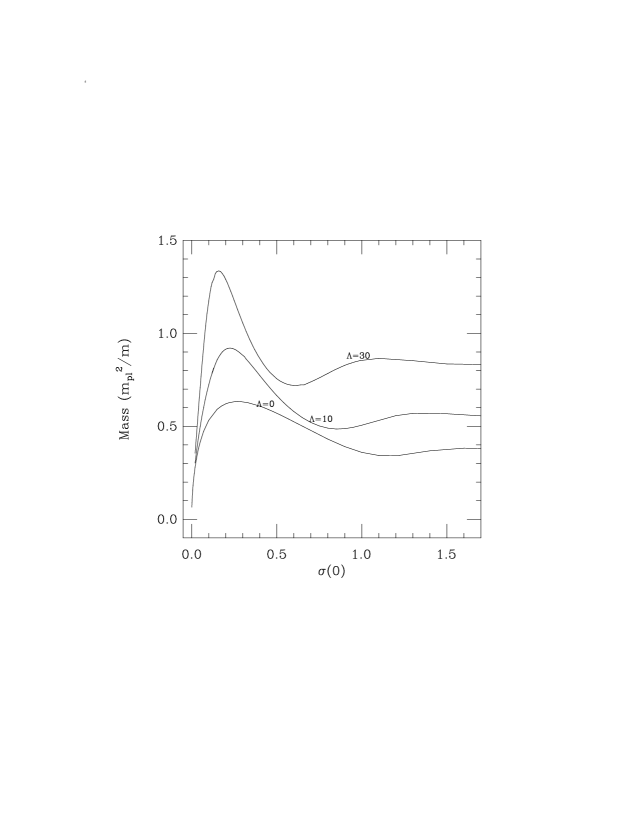
Figure 1: Mass profiles of ground state boson stars for different values of the self-coupling $\Lambda$ are shown. The increase in mass with $\Lambda$ is clear although the profiles are very similar.

Figure 2: Masses of zero-node, one-node and two-node boson stars without self-coupling are plotted as a function of central density. The maximum mass of one-node stars is $1.356\,M_{Pl}^{2}/m$ while the maximum mass for two-node stars is (as expected) greater at $2.095\,M_{Pl}^{2}/m$. The profiles are deceptively similar to their ground state counterparts. Excited state stars are inherently unstable irrespective of the branch they lie on, unlike ground state stars that can be termed stable or unstable depending on whether they lie on the branch to the left of the maximum mass or to the right respectively.

2.3.2 BD Case

Equilibrium configurations of boson stars in BD theory have been discussed in [52]. They used a modified version of the code we used to get equilibrium GR configurations. They added the BD terms to the equations as well as adding the BD scalar field. The equilibrium configurations in this case were those for which the boson field has the $e^{i\omega_{E}t}$ dependence in time as described before, while the metrics and the BD field are static. The value of the central BD field was not a free parameter but depended on its specified value at $\infty$. This was chosen to be zero to some tolerance. The equations were integrated for different values of the central lapse value for a given central boson field value and guessed central BD field value. The value of the Brans–Dicke field at the edge of the grid was checked against its expected value ($\sim\varphi_{\infty}+C/r$) to the predetermined tolerance. If it did not match the value of the central BD field was changed and the process repeated for different central lapse values until a match was found. Since these configurations were quite similar to the GR case the central lapse values were close to the GR values. For all self-couplings the BD particle number was very slightly smaller than the GR case while the mass was slightly lower for small values of self-coupling and slightly larger for higher values of self-coupling. This was true for both the ground state and excited state configurations.

2.3.3 Boson Halos

The equilibrium configurations are obtained (BD equations with $m=a=0$), from the equations

$$\sigma^{\prime}=\chi\;,$$ (90)

$$\chi^{\prime}=-\left[\frac{1}{r}+\frac{g^{2}}{r}\right]\chi-\frac{\sigma g^{2}}{N^{2}}\;,$$ (91)

$$g^{\prime}=\frac{1}{2}\,\left[\frac{g}{r}-\frac{g^{3}}{r}+\frac{\sigma^{2}\,r\,g^{3}}{N^{2}}+r\,g\,\chi^{2}\right]\;,$$ (92)

$$N^{\prime}=\frac{1}{2}\,\left[-\frac{N}{r}+\frac{N\,g^{2}}{r}+\frac{r\,g^{2}\,\sigma^{2}}{N}+r\,N\,\chi^{2}\right]\;.$$ (93)

Here we use the dimensionless variables $r=\omega{\bf r}$, $t=\omega{\bf t}$ and $\sigma=\sqrt{4\pi G\,}\phi$. These equilibrium configurations are characterized by static metrics although the fields themselves again have an $e^{i\omega t}$ dependence. Regularity at the center implies $g(r=0)=1$. The equilibrium configurations are characterized by saddle points in the density $\rho$, which might have some significance in stability issues. These systems are characterized by a two parameter family of solutions. Firstly, we can vary $\sigma(0)$, the central density and for each $\sigma(0)$ we can vary $N(0)$. This is effectively changing the frequency and for each value of the frequency of the system there is a configuration for which the dispersive effects cancel the gravitational effects. We have noticed an interesting feature of the mass function,

$$M(r)=\frac{r}{2}\left(1-\frac{1}{g^{2}}\right)\;,$$ (94)

where $g^{2}$ is the radial metric. If plotted at a given value of $r$ the profile is very similar to boson stars as shown in figure 3a. We also see the increase in mass linearly with radius for large $r$ in the relativistic case. Figure 3b shows mass versus radius for different central densities and a given value of $N(0)$.

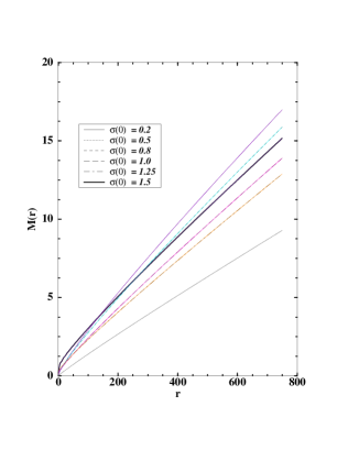
Figure 3: (a) Left: The mass profile of equilibrium configurations of massless scalar fields, are interestingly similar to the profiles of massive scalar fields and neutron stars. The mass for a given radius increases to a maximum with central density before it decreases with further increase in central density. However by calculating the particle number, we see no division into stable and unstable configurations at the peak. The particle number depends very sensitively on the initial value of the lapse function $N$, so that the clear cusp structure seen in the mass-particle-number diagram for boson stars cannot be derived here. (b) Right: The profiles are largely independent of radius although the mass itself increases with $r$.

Chapter 3 Numerical Evolution of Bosonic Objects in Spherical Symmetry

In the previous chapter we developed (from the action for a BD system with a matter Lagrangian that produces a scalar field equation for bosons, and for a spherically symmetric metric) the basic equations that govern the structure of an equilibrium boson star (see 2.1.1). The GR case was a special case of these with the parameter $a$ set to zero and discarding the BD field equation. (The BD field decouples from the physics). We now write down the evolution equations for the BD case. These of course include the time derivatives of the metric and the BD field. For convenience, so that we have no second time derivatives, we introduce new variables

$$\Pi_{\varphi} = {g\over N}\,\partial_{t}(r\,\varphi)\equiv{1\over\beta}\,\partial_{t}(r\,\varphi),$$ (1)

$$\Pi_{\Psi} = {g\over N}\,\partial_{t}(r\,\Psi)\equiv{1\over\beta}\partial_{t}(r\,\Psi),$$ (2)

where $\Psi=\sqrt{4\pi G_{*}}\phi$.

We thus get the field equations (for $\phi$, $\Psi$)

$$\partial_{t}(r\,\varphi) = \beta\,\Pi_{\varphi},$$ (3)

$$\partial_{t}\Pi_{\varphi} = (\partial_{r}\beta)\,\partial_{r}(r\,\varphi)+\beta\,\partial_{r}\partial_{r}(r\,\varphi)-(\partial_{r}\beta)\,(r\,\varphi)\,{1\over r}$$ (5)

$$-N\,g\,r~{}2\,\alpha\,e^{2a}\left[{1\over 2}\,\nabla_{\sigma}\Psi\,\nabla^{\sigma}\Psi^{\dagger}+2\,e^{2a}\,V(\Psi\Psi^{\dagger})\right],$$

$$\partial_{t}(r\,\Psi) = \beta\,\Pi_{\Psi},$$ (6)

$$\partial_{t}\Pi_{\Psi} = (\partial_{r}\beta)\,\partial_{r}(r\,\Psi)+\beta\,\partial_{r}\partial_{r}(r\,\Psi)-(\partial_{r}\beta)\,(r\Psi)\,{1\over r}$$ (8)

$$-2\,N\,g\,r\left[e^{2a}{dV(\Psi\Psi^{\dagger})\over d\Psi^{\dagger}}-\alpha\,\nabla_{\sigma}\Psi\,\nabla^{\sigma}\varphi\right].$$

where there are really two components for the second equation above (since we have a complex boson field). On each time slice we solve for the lapse $N$ by using the $rr$ component of the Einstein equation. However, instead of using the $00$ component to get the radial metric on each time slice it is more convenient to use this component to record the time development of the radial metric through the $0r$ equation (the momentum constraint equation). The momentum constraint and $G_{rr}$ equations are respectively

$$\partial_{t}g = N\,[\Pi_{\varphi}\,\partial_{r}\varphi+e^{2a}\,{1\over 2}\,(\Pi_{\Psi}^{\dagger}\,\partial_{r}\Psi+\Pi_{\Psi}\,\partial_{r}\Psi^{\dagger})],$$ (9)

$$\partial_{r}N = {N\over 2\,r}\,(g^{2}-1)+{N\,r\over 2}\left((\partial_{r}\varphi)^{2}+\Pi_{\varphi}^{2}\,{1\over r^{2}}\right.$$ (11)

$$\left.+e^{2a}\,\left[(\partial_{r}\Psi)\,(\partial_{r}\Psi^{\dagger})+\Pi_{\Psi}\,\Pi_{\Psi}^{\dagger}\,{1\over r^{2}}-2\,g^{2}\,e^{2a}\,V(\Psi\Psi^{\dagger})\right]\right).$$

Since $T_{00}$ is the energy density the $G_{00}$ equation is the Hamiltonian constraint equation. It is given by

$$2\,{\partial_{r}g\over g\,r}+{g^{2}-1\over r^{2}}={\Pi_{\varphi}^{2}\over r^{2}}+(\partial_{r}\varphi)^{2}+e^{2a}\,\left[{\Pi_{\Psi}\,\Pi_{\Psi}^{\dagger}\over r^{2}}+(\partial_{r}\Psi)\,(\partial_{r}\Psi^{\dagger})+2\,g^{2}\,e^{2a}\,V(\Psi\Psi^{\dagger})\right].$$ (12)

This is used to monitor the code by keeping track of the accuracy with which it is satisfied throughout the evolution. Orders of $10^{-5}$ or better are typical at the end of our runs.

3.1 Evolution Equations and Code

The equations that describe the evolution of the boson star in GR are given by those in (6)–(11) with the parameter $a$ set to zero, and again discarding the wave equation for the BD field. In order to finite-difference the derivatives, one must rely on well studied methods used in the study of linear differential equations, although we are in fact dealing with very non-linear systems. Our equations are of the hyperbolic form (wave equation) and we use a leapfrog method for evolution [51].

• Leapfrog Method

  • Consider a simple outgoing wave equation of the form

    $$\frac{\partial u}{\partial t}=-v\frac{\partial u}{\partial x}.$$ (13)

    Now take a one-sided differencing scheme for the time-derivative ($n$ representing the timestep and $j$ the position of a space coordinate)

    $$u_{j}^{n}=u_{j}^{n+1}-\frac{\partial u}{\partial t}\Bigg{|}_{j,n}\Delta t+O((\Delta t)^{2})$$ (14)

    $${\mathchoice{\hbox{{so }}}{\hbox{{so }}}{\hbox{{so }}}{\hbox{{so }}}}\frac{\partial u}{\partial t}\Bigg{|}_{j,n}=\frac{u_{j}^{n+1}-u_{j}^{n}}{\Delta t}+O(\Delta t).$$ (15)

    For spatial derivatives consider a second-order representation

    $$u_{j}^{n} = u_{j+1}^{n}-\Delta x\,u^{\prime}|_{j,n}+(\Delta x)^{2}u^{\prime\prime}+O((\Delta x)^{3})$$ (16)

    $$u_{j}^{n} = u_{j-1}^{n}+\Delta x\,u^{\prime}|_{j,n}+(\Delta x)^{2}u^{\prime\prime}+O((\Delta x)^{3})$$ (17)

    so that on subtracting the two equations

    $$u^{\prime}|_{j,n}=\frac{u_{j+1}^{n}-u_{j-1}^{n}}{2\Delta x}+O((\Delta x)^{2}).$$ (18)

    Thus this ‘Forward-Time Centered-Space’ scheme gives

    $$\frac{u_{j}^{n+1}-u_{j}^{n}}{\Delta t}=-v\left(\frac{u_{j+1}^{n}-u_{j-1}^{n}}{2\Delta x}\right).$$ (19)

    This scheme is unstable as shown by Von Neumann stability analysis. Consider the coefficient $v$ to be slowly varying enough to be considered constant. Now consider eigenmodes of the difference equation of the form $u_{j}^{n}=\xi^{n}e^{ikj\Delta x}$ so that

    $$\xi-1=-\frac{v\Delta t}{\Delta x}\,i\,\sin(k\Delta x).$$ (20)

    The time dependence of the eigenmodes grows like $\xi^{n}$ and since $|\xi|=\sqrt{1+(\frac{v\Delta t}{\Delta x})^{2}\sin^{2}(k\Delta x)}>1$ this instability grows and renders the scheme unstable.

    So instead one uses a $staggered$ $leapfrog$ method using centered-time and centered-space derivatives.

    $$\frac{u_{j}^{n+1}-u_{j}^{n-1}}{\Delta t}=-v\left(\frac{u_{j+1}^{n}-u_{j-1}^{n}}{\Delta x}\right).$$ (21)

    Now we get a quadratic equation for $\xi$ with a solution $|\xi|=1$ for any $\frac{v\Delta t}{\Delta x}<1$. Thus there is no growth of instability or amplitude dissipation  [51, 37]. It is called a leapfrog scheme because the time derivative terms are on odd time slices while the time levels in the space derivative terms are on even time slices.

    When one has second-order time derivatives (as we do) it is more appropriate to redefine the first time derivative in terms of another variable ($\pi=\frac{g}{N}\frac{\partial(r\psi)}{\partial t}$) that is then given on the $n+\frac{1}{2}$ steps.

The two components of the equilibrium scalar field have components $\Psi_{1}$ with time dependence as $\cos(\omega_{E}t)$ and $\Psi_{2}$ with time dependence as $\sin(\omega_{E}t)$. Thus quite generally at $t=0$ we set the field $\Psi_{2}=0$. Our equilibrium code calculates the initial field configuration $\Psi_{1}$ and the metric components as functions of $r$. This is the initial data for the evolution code. The first spatial derivatives of the metrics and fields are then determined by using $f^{\prime}\Delta x=a\left(f(x+3\Delta x)-f(x-3\Delta x)\right)+b\left(f(x+2\Delta x)-f(x-2\Delta x)\right)+c\left(f(x+\Delta x)-f(x-\Delta x)\right)$. The coefficients $a$, $b$ and $c$ are determined ($a=1/60$,$b=-9/60$, $c=45/60$) from the conditions that the coefficient of the first derivative of the Taylor expansion be $\Delta x$ and the third and fifth derivative coefficients be zero. This makes $f^{\prime}$ sixth order accurate since the even derivatives automatically vanish. In order to get sixth order accuracy in the second derivatives the form above is applied for $f^{\prime\prime}(\Delta x)^{2}$ this time with every $f(x-s)$ and $f(x+s)$ added rather than subtracted so odd derivatives vanish. The coefficients are then determined ($a=2/180$, $b=-27/180$ , $c=490/180$). At the last but one grid point though one only has terms to second order accuracy.

The metrics and fields have vanishing first derivatives at the origin. From the equations it is clear their parities are conserved. A pair of fictitious points corresponding to negative $r$ are set up. The code evolves $r\psi$ and $\pi$ which are antisymmetric about the origin. The derivative of $r\psi$ at the origin is $\psi$ and that is how we determine it. The radial metric at the origin is unity but the lapse is not prescribed there. Instead we choose to fix the lapse at the outer boundary and integrate inwards on each slice using a fourth order RK method. Rather than integrate the Hamiltonian constraint equation on each slice to determine $g$ we monitor its evolution from time step to time step. We only determine the boundary value of $g$ from the Hamiltonian constraint equation.

The outer region of the system is the low field region and the mass of the system can be determined using the value of the radial metric there.

$$M=\lim_{r\rightarrow\infty}\frac{r}{2}\,\left[1-\frac{1}{g^{2}(r)}\right].$$ (22)

The outer boundary condition on the fields is an outgoing wave condition. If in the asymptotic region the field is of the form $\sim e^{i({\bf k.r}-\omega t)}$, then this results in the condition (from the KG equation)

$$\frac{k^{2}}{g^{2}} = \frac{\omega^{2}}{N^{2}}-m^{2},$$ (23)

$${\mbox{g}iving}\quad k = \frac{g\,\omega}{N}(1-\frac{1}{2}\,m^{2}\,\frac{N^{2}}{\omega^{2}}+...),$$ (24)

which can be written (in terms of the fields and dimensionless units of the code) as

$$\dot{\pi}=-\beta\pi^{\prime}-\frac{N^{2}}{2}r\psi,$$ (25)

where $\beta=\frac{N}{g}$. This eliminates first order reflections off the grid. In order to remove higher-order reflections, we add a “sponge” in the outer region of the grid to absorb reflections. To the $\dot{\Pi}$ equation (8) we add a damping term at the edge of the grid. This “sponge” is effectively like adding a potential term that is proportional to $k+\omega$ for an incoming wave and proportional to $\omega-k$ for an outgoing wave. Thus it forms a potential barrier against incoming radiation. This sponge is smoothly phased in from some point $r(j)$ out to the edge of the grid. The width of the sponge is of the order of the wavelength of the scalar radiation.

3.2 Nature of the Perturbations

We study the dynamical properties of the boson stars by perturbing the equilibrium field distribution. The accretion or annihilation of scalar particles is simulated by the addition of field in the outer regions of the star or by decreasing it in denser regions of the star respectively. Another type of perturbation that has been studied is changing the $\dot{\psi}_{1}$ and $\dot{\psi}_{2}$ of the equilibrium configuration. This perturbation changes the kinetic energy density distribution. In either case the changes in the metric functions $g$ and $N$ are determined by the constraint equations and the polar-slicing condition. That is, we reintegrate the Hamiltonian constraint and lapse equations of (11) and (12) on the initial time slice. The magnitude and the length scale of the perturbations can be chosen arbitrarily. The perturbations are always spherically symmetric.

3.3 Results and Conclusions for 1D Boson Stars with Self-Coupling

• Ground State Results

An equilibrium configuration of boson stars when perturbed reacts to these perturbations in a myriad of ways. As discussed before, in the works of Pang and Lee [3], ground state boson stars without self-coupling on the $S$ branch have very specific quasinormal modes of oscillation under infinitesimal perturbations. In  [55] the mass function is plotted against radius for a given particle number. The curve is seen to have a “well” with a minimum at the exact equilibrium mass corresponding to that particle number. For any other given mass at that particle number there are oscillating regimes from a minimum to a maximum radius. In a numerical scenario we are in a position to test more general and realistic perturbations. While we do study the effects of infinitesimal perturbations (by applying perturbations for which the mass change from equilibrium is less than $0.1\%$.) larger perturbations are also analyzed. The effects of larger perturbations cannot be studied analytically using perturbative methods. From the former we get quasinormal modes of oscillations, while from the latter we get scalar radiation that results in mass losses in these stars followed by their eventual settling to stable configurations of lower mass, their collapse to black holes, or their total dispersal. Once perturbed the metric equations are reintegrated to get consistent metrics for those new initial configurations. Thereafter the system is allowed to evolve under the evolution equations.

• $S$ Branch Stars

In the case of a free field ($\Lambda=0$ case) a perturbed $S$-branch star oscillates with a definite frequency, losing mass through bursts of scalar radiation at each expansion. It finally settles to a new $S$-branch configuration of lower mass. Here the effect of a self-interaction term on this behavior is examined. In Fig. 1 a typical example of the perturbed field configuration, and radial metric, of a star with $\Lambda=10$ and a central density of $\sigma(0)=0.1$ is shown. This star has been perturbed by accretion of scalar particles in a region of lower density. Its evolution is detailed below.

Fig. 2 shows the radial metric as a function of distance for the same configuration at various times. The labels $A,B,C,D$ correspond to times (in units of the inverse of the underlying scalar field frequency) $t=192,\,\,306,\,\,391,$ and $505$ respectively. The positions of the peaks are labeled $R_{0},\,\,R_{A},\,\,R_{B},\,\,R_{C},$ and $R_{D}$, where $R_{0}$ is the position of the initial unperturbed peak. Here $R_{0}=7.95,\,\,R_{A}=8.55,\,\,R_{B}=6.6,\,\,R_{C}=8.2$ and $R_{D}=6.65,$ where the length scale is in terms of the inverse mass of the boson. The oscillations are shown clearly in Fig. 3 which is a plot of the maximum value of the radial metric as a function of time. The point where this function is a maximum corresponds to the core of the star contracting to its minimum size in a cycle. Similarly, the maximum radial metric starts to decrease as the star expands. At each expansion the star loses mass through scalar radiation. The oscillations damp out in time as the star starts settling down to the new configuration. A plot of mass vs. time is shown in Fig. 4. The emission of scalar radiation decreases as the oscillations damp out, as can be seen from the figure. The slope of the curve steadily decreases as the star starts settling down to its new lower-mass configuration. The mass is measured at the inner edge of the sponge using (22). Exact details of the curves have some dependence on the sponge parameters but the basic results are the same.

A characteristic of the boson star that might be important for its potential observation and identification is its fundamental oscillation frequency which can be determined from Fig. 5. We found $f=1/(199\,N(\infty))=4.7\times 10^{-3}$. The oscillation frequencies for a large number of S-branch stars have been compiled in this way. Fig. 5 shows a plot of the oscillation frequency versus mass for many slightly perturbed configurations (masses within 0.1% of the unperturbed mass.) As the mass increases, the frequency increases and then drops down as the transition point ($dM/d\sigma(0)=0$) is approached, signalling the onset of instability. This is seen for both the non self-interacting as well as the self-interacting case. These quasinormal modes of oscillation characterize $S$-branch stars. The point of transition from the $S$ to the $U$ branch corresponds to a zero of the oscillation frequency.

For a given mass higher $\Lambda$ $S$-branch stars have a lower oscillation frequency than similar mass lower $\Lambda$ stars, unless one is near the transition point of the lower $\Lambda$ configuration. This is not too surprising, since for a given mass the radius of the star increases with increasing $\Lambda$. We have seen this trend even for $\Lambda$ values as high as $1600$ (see discussion on high $\Lambda$ stars in section (3.3.2)). However since the maximum mass of higher $\Lambda$ configurations is greater than that of lower $\Lambda$ configurations their maximum oscillation frequency could be greater than that for lower $\Lambda$ stars. (This can be understood as a size effect: on the $S$-branch, higher mass stars are smaller and have higher frequencies.) This can be seen in Fig. 5 . The maximum oscillation frequencies of $\Lambda=5$ and $\Lambda=10$ configurations are higher than that of the $\Lambda=0$ case. As the stars get much larger, though, the highest frequency starts to decrease. For example the maximum frequency for $\Lambda=30$ stars is less than that of $\Lambda=15$ stars which is itself lower than that of the $\Lambda=10$ case. A perturbation calculation for the high $\Lambda$ case is presented in section (3.3.2) to show the dependence of the quasinormal mode frequencies on $\Lambda$ for high $\Lambda$ configurations. The frequency is then proportional to the inverse of the square root of $\Lambda$. Thus as the stars become extremely large they oscillate less and less rapidly and it is no longer feasible to evolve them numerically in our code. (The time step used in the numerical simulation cannot be increased as it is determined by the intrinsic oscillation time scale of the scalar field, which is many orders of magnitude shorter than the oscillation time scale of the whole star for these cases.)

The quasinormal mode curves are also useful in determining the evolution of strongly perturbed $S$-branch stars and the final configurations they could settle into. A perturbed star loses mass and settles to a final configuration corresponding to some position on the solid line in the figure. In Fig. 6 we single out the $\Lambda=10$ curve and plot the evolution of the $S$-branch star discussed above. The points $P1$, $P2$, and $P3$ show the route to a new configuration. These points correspond to times $t=0$, $1200$, and $4800$ respectively. By extrapolating this line to where it meets the $\Lambda=10$ curve one could expect a final mass of about $0.76\,M_{Pl}^{2}/m$ .

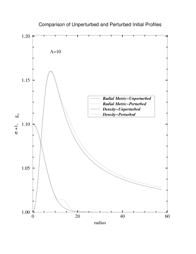
Figure 1: Comparison of a strongly perturbed ground state $\Lambda=10$, $S$-branch star [$M=0.781\,M_{Pl}^{2}/m,\sigma(0)=0.1$] to the unperturbed configuration [$M=0.722\,M_{Pl}^{2}/m$]. The solid lines correspond to the unperturbed configuration and the dashed ones to the perturbed star. The perturbation shown corresponds to the addition of scalar field $\sigma$ at $t=0$.

Figure 2: The evolution of the radial metric $g_{rr}=g^{2}$ for the configuration shown in the previous figure. The initial perturbed configuration labeled $t=0$ and unperturbed configuration are shown. $A,\,\,B,\,\,C,$ and $D$ correspond to times $t=192,\,\,306,\,\,391,$ and $505$ respectively. The positions of the peaks for these times are labeled $R_{A},\,\,R_{B},\,\,R_{C},$ and $R_{D}$.

Figure 3: The peak value of the perturbed radial metric is plotted over a long time ($6000\,\hbar/mc$). The points labeled $A$, $B$, $C$, and $D$ correspond to the same labels in the previous figure. The oscillations decay in time.

Figure 4: The total mass of the star is plotted as a function of time. The mass loss through scalar radiation decreases in time as the oscillations start damping out.

Figure 5: The oscillation frequencies of different ground state boson star configurations are plotted as functions of mass, for $\Lambda=0$, $5$, $10$, $15$, $30$, $100$, and $200$. The curves are obtained by slightly perturbing (perturbed mass within $0.1\%$ of the unperturbed mass) $S$-branch stars. They reach a peak and then drop down at the approach of the maximum mass allowed for a given $\Lambda$, signalling a transition from stability to instability.

Figure 6: The highly perturbed $\Lambda=10$ $S$-branch star has an oscillation frequency below the $\Lambda=10$ solid line. Its movement towards the solid line is shown through points $P1$, $P2$, and $P3$ corresponding to times 0, 1200, and 4800 ($\hbar/mc$) respectively.

• $U$-branch Stars

Ground state $U$-branch stars (with or without self-coupling) can migrate to the $S$ branch under certain perturbations. In general they are unstable and cannot settle into new configurations on the same branch. In  [55], with the aid of catastrophe theory, the instability of these unstable stars is also discussed. Their conclusion regarding unstable boson stars is that they disperse or collapse. However we also demonstrate the presence of migrations of these stars to configurations on the $S$ branch. This is due to our perturbations being more general, allowing for changes in mass and particle number, whereas they keep them strictly constant.

Figs. 7-9 show a migrating $\Lambda=30$ star whose unperturbed overall field density $\sigma$ has been decreased by about 10%. Fig. 7 shows the behavior of the radial metric in time as a function of radius. It oscillates about the final $S$-branch configuration that it will settle into. This final state is shown on the plot as a dark line. Fig. 8 shows the maximum radial metric as a function of time. The star initially expands rapidly as it moves to the $S$-branch. This can be seen from the sharp drop in the radial metric. Once it moves to the stable branch, it oscillates about the new configuration that it is going to settle into. Fig. 9 shows the mass of the star as a function of time. It loses mass at each expansion losing less and less mass at each subsequent expansion and the curve gets smoother and smoother as it settles to its final state.

Fig. 10, which shows the oscillation frequency as a function of mass for $\Lambda=30$, can be used to predict the end point of migration. Points $Q1$, $Q2$, $Q3$, and $Q4$ show the migration of this star. These correspond to times of 500, 1000, 2000, and 3500. The oscillation is clearly damping out. The final configuration it is expected to settle down to is shown as a dot and corresponds to a stable star of central density $\sigma(0)=0.0817$ with a mass of $1.037\,M_{Pl}^{2}/m$. This example is typical of a number of simulations of $U$-branch ground state configurations with self coupling.

For higher central density stars on the $U$-branch, the mass versus central density curve has a second, gentler peak, similar to the white dwarf neutron star situation. One might suspect that this corresponds to another stable and unstable branch respectively. However we find that configurations on both sides of the peak are unstable. These configurations always disperse upon perturbation, consistent with the fact that they have $M\,>\,N\,m$, where $M$ is the mass of the star and $N\,m$ is the number of bosons multiplied by the mass of an individual boson.

Figure 7: The radial metric $g^{2}=g_{rr}$ of a perturbed $U$-branch ground state star is shown at various times. The curves $1\,\,,2,\,\,3,\,\,a,\,\,b,\,\,c$, and $d$ correspond to times $t=10,\,\,20,\,\,30,\,\,340,\,\,440,\,\,540$, and $640$. The unperturbed star has a central density $\sigma(0)=0.23$ and a self coupling parameter $\Lambda=30$. The initial equilibrium metric configuration has also been shown. The initial field density of this star has been lowered by about $10\%$. The $t=0$ curve corresponds to the initial perturbed radial metric. In the asymptotic region $g^{2}$ is not oscillating but monotonically decreasing due to the mass loss.

Figure 8: The maximum value of the radial metric is plotted as a function of time. The initial sharp drop in the radial metric is due to the expansion of the star as it proceeds to the stable branch. There it oscillates about the new stable configuration that it will settle into. This corresponds to a star of mass $M=1.037\,M_{Pl}^{2}/m$ (whose metric configuration has been shown in the previous figure as a dark line). The points $a$ and $c$ correspond to two minima in the peak of $g_{rr}$ which occur when the core of the star reaches its local maximum size. Likewise the maxima in the peak of $g_{rr}$ at $b$ and $d$ correspond to the core of the star reaching its local minimum size.

Figure 9: The mass is plotted against time. The mass loss through scalar radiation at each expansion of the core (corresponding to the maximum radial metric reaching a minimum) decreases in time as the oscillations damp out.

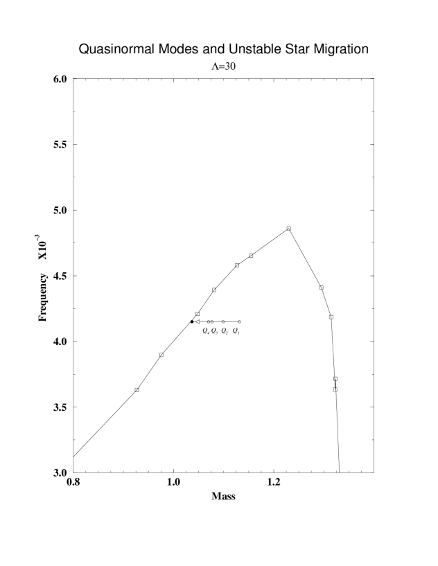
Figure 10: The migration of the $U$-branch star considered in the previous figure is shown after the star has moved to the $S$-branch. Points $Q1$, $Q2$, $Q3$, and $Q4$ correspond to times 500, 1000, 2000, and 3500 ($\hbar/mc$) respectively. Here too the mass loss decreases in time and the star finally settles to a stable configuration.

3.3.1 Excited States

The similarity of mass profiles of excited boson stars to their ground state counterparts, (Fig. 2) might lead one to expect stable and unstable configurations to the left and right of the maximum mass respectively in analogy with ground state configurations. However, our numerical studies show that the excited boson star configurations on both sides of the peak are inherently unstable except that the time scales for instability are different. If they cannot lose enough mass to go to the ground state they either become black holes or totally disperse. This occurs even if no explicit perturbations are put in the numerical evolution other than those introduced by the finite differencing error in the numerical integration. We have also carried out perturbations that correspond to scalar particles falling onto the star, or those that decrease the scalar field strength at the center point (corresponding to scalar particles decaying through some channel). The instability shows up in all cases studied. We note that this instability is $NOT$ in contradiction with the result of [53], which concluded that $S$ branch excited states are stable under infinitesimal perturbations that strictly conserve $M$ and $N$, (where $M$ is the mass of the star, $N$ the number of bosons and $m$ the boson mass.) Our result of instability under generic perturbation is consistent with the studies of $\Lambda=0$ stars under infinitesimal perturbation [3]. The presence of a self-coupling term increases the time scale of instability but the essential pattern remains the same. Fig. 11 shows a perturbed 1-node star (whose mass has been reduced by about $8\%$ to $0.9\,M_{Pl}^{2}/m$ by a perturbation) making a transition to the ground state although the mass is greater than the maximum ground state mass of $0.633M_{Pl}^{2}/m$. A substantial amount of scalar radiation is emitted in the dynamical evolution, which brings the mass below the critical value. The evolution of the radial metric function is shown. That there are two peaks at $t=0$ is indicative of a first excited state. One of the peaks disappears gradually as the star goes to the ground state branch. The star then oscillates about the ground state configuration that it will finally settle into. In Fig. 12 a three-node configuration with a total mass of of $0.92M_{Pl}^{2}/m$ is shown going to the ground state branch, after radiation by scalar waves carries off the excess mass and kinetic energy. The plot shows the density function against the radius and time of evolution. By the density function we mean density $\rho$ multiplied by $r^{2}$, that is, the mass per $dr$ at radius $r$. The density function, $\rho\,r^{2}$, has $n+1$ maxima for an $n$ node star and hence here we have four sets of lines initially. At the end of the simulation, we see that it settles down to a ground state configuration with small oscillations with ever decreasing amplitude. For these simulations of low central density stars we put in an explicit perturbation to the equilibrium configuration since otherwise the instability time scales are extremely long.

For stars with higher central density, there is a critical density above which the stars cannot lose enough mass to go to the ground state but collapse to black holes. In our numerical simulation for one node stars this critical density is $\sigma(0)=\sigma_{2}=0.048$. As the central density is increased the kinetic energy of the highly compressed initial equilibrium configuration is increased and the star first expands before the eventual collapse to a black hole. As the central density further increases towards the $M=N\,m$ point the expansion phase becomes longer. In Fig. 13 we show the density function ($\rho r^{2}$) against radius at various times for 4 configurations (an $S$-branch configuration with $\sigma(0)=0.1$, and three $U$-branch configurations of central densities $\sigma(0)=0.3$, $\sigma(0)=0.4$, and $\sigma(0)=0.5$). The initial configurations are the equilibrium ones without any explicit perturbation (except those introduced by the discretization used in the numerical simulations). The first frame shows the $S$-branch star radiating a little as it almost makes a transition to the ground state. However it cannot sustain this state for long and it collapses to a black hole. The decay time decreases in the case of a $U$-branch stars of central density $0.3$ and $0.4$. However for the $\sigma(0)=0.5$ star, the star is clearly getting more diffuse than the previous ones. It goes through an expansion phase initially although it finally collapses to a black hole. Configurations with $\sigma(0)>0.54$ have $M>N\,m$. They do not collapse to black holes but disperse to infinity. Next we turn to a study of instability time scales. In simulations where a black hole will form, the imminent development of an apparent horizon leads to a rapid collapse of the lapse due to the polar slicing used in the evolution. We take the time of collapse of the lapse at the origin to $\sim 10^{-6}$ of its initial central value to be the approximate time for formation of the black hole. Fig. 14 shows this time scale for a 1-node star without self coupling. We plot the decay time scales of first excited state stars as a function of central field density. Again no explicit perturbation is applied in these evolutions other than the discretization error in the simulation. In order to make a fair comparison of the time scale due to such a perturbation we cover the radius of the star in all cases by the same number of grid points. The maximum ground state mass for stars without self coupling is around 0.633 $M_{Pl}^{2}/m$. This corresponds to a central density of $\sigma_{1}=0.021$ for a one-node star. We mentioned earlier that stars with central densities below $\sigma_{2}=0.048$ (mass of $0.91M_{Pl}^{2}/m$) lose enough mass and move to the ground state. Beyond that and up to the point $M=N\,m$ they collapse to black holes, while stars with $M>Nm$, corresponding to a central field density of $\sigma(0)>0.541$, disperse to infinity. The time by which collapse takes place to a black hole decreases with increasing central density along the $S$ branch. This trend continues for a while into the $U$ branch (starting at $\sigma=0.25$ until $\sigma\sim 0.4$), but as one approaches the $M=N\,m$ point the stars lose a significant amount of matter to infinity before they collapse to black holes and evolve on a longer time scale. For example, a star of central density $0.5$ has an initial radius of $r\sim 9$. (Remember that the radius of the star is defined as the radius which contains $95\%$ of the mass of the star.) Its radius increases to as much as 115, more than an order of magnitude, before it starts collapsing. The dispersion time scales of a couple of typical examples of stars for $M>Nm$ which disperse to infinity (instead of collapsing to a black hole) are also shown on the figure. To give a sense of the instability time scales of these configurations we take the time scale to be the time by which these stars disperse to ten times their original radii. This time drops drastically for stars with $M\gg Nm$.

Next we turn to the case of $\Lambda\neq 0$. Fig. 15 demonstrates black hole formation for a $\Lambda=30$ star in the first excited state, with a central density $\sigma(0)=0.1$. This star had an initial radius of about 20.7 where the radius is again defined as that containing $95\%$ of the mass. The lapse finally collapses towards zero indicating that an apparent horizon is about to form. The time scale of collapse to the black hole was around 1985 compared to a time scale of less than 800 for a $\sigma(0)=0.122$ star of similar radius without self-coupling which is shown in Fig. 16. This is to be expected as the $\Lambda$ term represents a repulsive force. The collapse time is again defined by the lapse collapsing to $10^{-6}$ of its original value at $r=0$.

We now turn to the evolution of a highly excited state. In Fig. 17 we show the initial field configuration of a star containing five nodes. For a five-node star the density has a central maximum, and then five local maxima, each subsequent one smaller than the one preceding it. This star is then evolved without any perturbation except those introduced by the discretization error of the numerical evolution. In Fig. 18 we show a contour plot of the evolution of the density function in time: $\rho\,r^{2}$ has $n+1$ maxima for an $n$ node star and hence here we initially have six sets of lines centered at dimensionless $r=5,\,\,13,\,\,35,\,\,52$, and $75$ respectively. This star has central density $\sigma(0)=0.075$ and it collapses to a black hole after a long evolution. In the process we see intermediate states with fewer numbers of nodes.

For comparison, in Fig. 19 we show the contour plot for the five-node star up to a time of $t=1000$, at which time it has decayed into a four-node state, against the equilibrium density function of a four-node star with central density $\sigma=0.06$. Very clearly the maxima are at similar radii (although the size of the peaks are somewhat different).

This feature, that of nodes disappearing and the star cascading through lower excited states, is characteristic of the decay of higher excited states of boson stars. Although in this particular case and at this particular time the decaying star is close to a specific lower excited state, in general the decaying star is (roughly speaking) a combination of lower excited configurations. This is similar to the decay of atoms in excited states. However, we note that for the “gravitational atom”[54] there is no exact superposition, due to the intrinsic non-linearity of the system.

Figure 11: The transition of a first excited state star to the ground state is shown. Here the radial metric is plotted against radius for various times starting from $t=0$ and then for $t_{a}=250$, $t_{b}=500$, $t_{c}=1245$, $t_{d}=4000$, $t_{e}=5000$, $t_{f}=5505$, $t_{g}=6000$, and $t_{h}=6370$. The initial unperturbed and perturbed configurations are shown. (The perturbed configuration has the lower second peak.) The initial mass of the star was $M=0.901\,M_{Pl}^{2}/m$ after perturbation. The radial metric initially has two peaks indicative of a one-node configuration. As the star evolves and goes to the ground state one peak disappears. This can be seen in the curves from $t_{c}$–$t_{h}$. Once on the ground–state branch it oscillates and finally settles into a stable ground–state configuration.

Figure 12: The transition of a three-node configuration of mass $0.91\,M_{Pl}^{2}/m$. This star loses enough mass during the course of its evolution to move to the ground state.

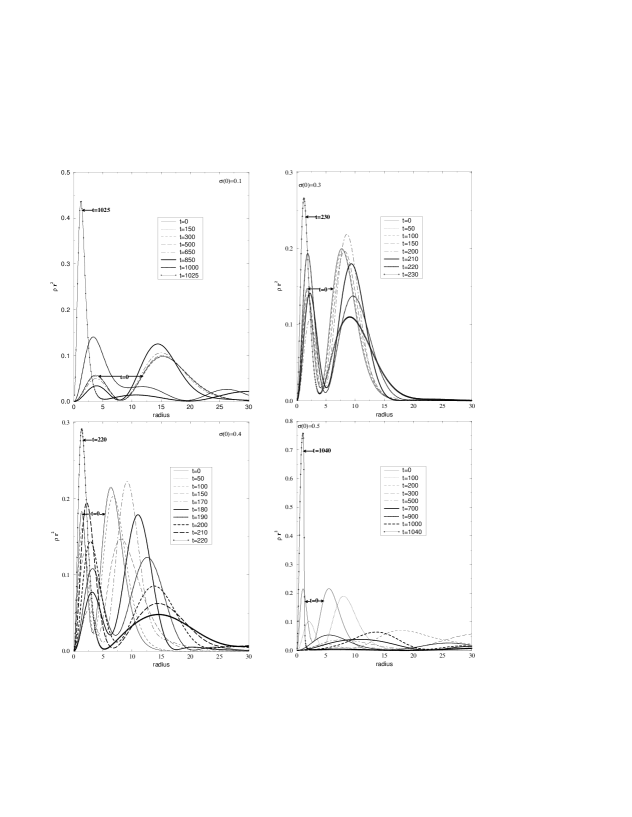
Figure 13: A comparison of the manner of black hole formation of four excited state configurations. The first frame is an $S$ branch star of central density $\sigma(0)=0.1$, that tries to go to the ground state but fails to. As the central density increases, decays to black holes occur on a shorter time scale. A plot of the collapse of a $U$-branch star of central density $\sigma(0)=0.3$ is shown in the next frame. Stars get more diffuse as one moves farther along the $U$ branch. A star of central density $0.4$ (shown in the third frame) has a decay time close to the previous one. Decay times then start to increase. A star of central density $0.5$ (close to the point $M=N\,m$ with $\sigma(0)\sim 0.541$) disperses to over ten times its radius before collapsing to a black hole.

Figure 14: The decay time to black holes is plotted as a function of central density, for one-node configurations (first excited states) of boson stars without self coupling. Perturbations are due only to the finite differencing effects of the numerical scheme. To make the comparisons meaningful the $95\%$ mass radius (which is our definition for radius of a star) of every configuration considered was covered by the same number of grid points. Configurations for which the central density $\sigma(0)<\sigma_{2}$ move to the ground state. The central density $\sigma_{1}$ corresponds to a mass $M=0.633\,M_{Pl}^{2}/m$, which is the maximum mass of a ground state boson star. The decay time decreases with increasing $\sigma(0)$ and this continues even for $\sigma(0)>0.25$ which is the transition point from the $S$-branch to the $U$-branch. The decay time then starts to increase as one approaches the $M=N\,m$ point corresponding to a central density $\sigma(0)=0.541$, beyond which the stars disperse to infinity rather than becoming black holes. The dispersion times of two such stars to ten times their original radius ($95\%$ mass radius) are also shown on the figure.

Figure 15: The evolution of the metric function $N^{2}=-g_{tt}$ for a $\Lambda=30$, $\sigma(0)=0.1$ boson star in the first excited state, without any explicit added perturbation, is shown. The configuration lies on the $S$-branch and has an initial mass $M=1.743\,M_{Pl}^{2}/m$. The various time slices correspond to times $t=0$, $t_{a}=1060$, $t_{b}=1950$, and $t_{c}=1985$. The lapse function collapses as an apparent horizon is approached, signaling the formation of the black hole. (This is indicative of an inherent instability of the excited states).

Figure 16: The evolution of the metric function $N^{2}=-g_{tt}$ for a $\Lambda=0$, $\sigma(0)=0.122$ boson star in the first excited state, without any explicit perturbation added, is shown. The configuration lies on the $S$-branch and has an initial mass $M=1.23\,M_{Pl}^{2}/m$. The various time slices correspond to times $t=0$, $t_{a}=450$, $t_{b}=720$, $t_{c}=750$, and $t_{d}=770$. This star has a radius of $20.7$ which is about the same as that of the configuration shown in the previous figure. Again, the lapse function collapses when an apparent horizon is approached, as a black hole is being formed. The time scale of collapse is much less than for the $\Lambda=30$ case in the previous figure.

Figure 17: The initial field configuration of a five-node star. The field has five nodes or extrema. The absolute value of each extremum is clearly smaller than the one preceding it.

Figure 18: A contour plot of a perturbed five-node star that decays into a black hole showing $\rho\;r^{2}$ as a function of distance (vertical axis) and of time (horizontal axis) is shown. The density $\rho$ is highest at the origin and has five other local maxima, each smaller than the previous one. The value of the maxima at the end are very small compared to the earlier ones, and to enhance the features $\rho\;r^{2}$ rather than just $\rho$ is shown in the plots. Each set of lines represents the maxima of $\rho\;r^{2}$ and the number of lines in a set gives an indication of the height of the maximum. This particular configuration has a mass $M=3.07\,M_{Pl}^{2}/m$. This star cascades through an intermediate four-node state (around $t=1000$) before proceeding to form a black hole. Cascades are characteristic of excited boson star decays, similar to atoms in excited states going through intermediate states when decaying to the ground state.

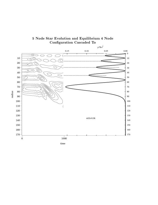
Figure 19: The equilibrium density function of a four-node star of central density $\sigma=0.06$ (right frame) is placed alongside the contour plot of the five-node star described in the previous figure up to a time of $t=1000$ when it has decayed into a four-node state (left frame). This plot shows that the transition of the five-node star is to a perturbed four-node state close to the one shown before it continues its evolution to a black hole.

Whenever we report black hole formation, we are of course talking about imminent formation since our highly singularity-avoiding polar slicing condition causes the lapse to collapse as soon as an apparent horizon forms. However taking the data just before such formation, and evolving it with a 3D code with maximal-slicing has allowed us to confirm that a black hole indeed forms.

3.3.2 Very High $\Lambda$ Configurations

While calculating the eigenvalue frequency for the equilibrium boson star it is found that it gets increasingly difficult to calculate the eigenvalue as the value of $\Lambda$ gets large, because the equations become very stiff. There are two scales to the problem: a scale of slow variation of the field inside a certain radius (related to $\Lambda$) followed by rapid decay outside it. This produces an effective surface layer to the star making it similar to neutron stars. It turns out that the large $\Lambda$ limit can be treated using a set of approximate equations that are exact in the $\Lambda=\infty$ limit [6]. By making the following change of variables:

$${\bar{r}}=\frac{r}{\sqrt{\Lambda}},\quad\quad{\bar{\sigma}}=\sqrt{\Lambda}\,\sigma$$ (26)

the equilibrium equations reduce to

$$\frac{1}{\Lambda}\,{\bar{\sigma}}^{\prime\prime}=-\frac{1}{\Lambda}\,\left[\frac{1}{{\bar{r}}}+\frac{g^{2}}{{\bar{r}}}-{\bar{r}}\,g^{2}\,{\bar{\sigma}_{0}}^{2}\right]\,{\bar{\sigma}^{\prime}}-\frac{1}{\sqrt{\Lambda}}\,\left[\frac{1}{N^{2}}-1\right]\,{\bar{\sigma}_{0}}\,g^{2}+\frac{1}{\sqrt{\Lambda}}\,(g^{2}\,{\bar{\sigma}_{0}^{3}}),$$ (27)

$$g^{\prime}=\frac{1}{2}\,\left[\frac{g}{{\bar{r}}}-\frac{g^{3}}{{\bar{r}}}+{\bar{\sigma}_{0}}^{2}\,{\bar{r}}\,g^{3}\,\left[1+\frac{1}{N^{2}}\right]+\frac{1}{\sqrt{\Lambda}}\,{\bar{r}}\,g\,{{\bar{\sigma}_{0}^{\prime 2}}}+\frac{1}{2}\,(g^{3}\,{\bar{r}}\,{\bar{\sigma}_{0}^{4}})\right]$$ (28)

$$N^{\prime}=\frac{1}{2}\,\left[-\frac{N}{{\bar{r}}}+\frac{N\,g^{2}}{{\bar{r}}}+\frac{{\bar{r}}\,g^{2}\,{\bar{\sigma}_{0}}^{2}}{N}\,(1-N^{2})+\frac{1}{\sqrt{\Lambda}}\,{\bar{r}}\,N\,{\bar{\sigma}_{0}^{\prime 2}}-\frac{1}{2}\,g^{2}\,N\,{\bar{r}}\,{\bar{\sigma}_{0}}^{4}\right].$$ (29)

where the primes refer to differentiation with respect to ${\bar{r}}$. In the limit of $\Lambda=\infty$, one can keep terms to leading order in $\frac{1}{\sqrt{\Lambda}}$ in (27) –(29). In particular (27) reduces to an algebraic constraint

$$N=({\bar{\sigma}}^{2}+1)^{-\frac{1}{2}}.$$ (30)

However, we note that this is valid only for a ground state configuration. For a state with nodes it would not be reasonable to neglect derivative terms compared to terms proportional to ${\bar{\sigma}}$, because it is zero at every node.

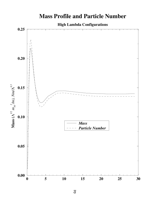
Figure 21: The mass of a high $\Lambda$ star generated from the approximate equations is plotted as a function of $\bar{\sigma}$ ($\sigma/\Lambda^{\frac{1}{2}}$). It shows the same basic structure as the profiles generated for low $\Lambda$ using the exact equations. The peak is at about $0.22\Lambda^{1/2}M_{Pl}^{2}/m$, which means that to achieve $0.1M_{\odot}$ we would have to take $\Lambda$ of order $10^{38}$. This would be a very large star to evolve numerically. Also plotted is $N\,m$ ($N$ is the particle number and $m$ the mass of a boson). The crossing point of the two curves represents transition from negative to positive binding energy.

To get an estimate of the accuracy of the high $\Lambda$ approximation we compare the solution using the approximate equation for high $\Lambda$ to the brute force numerical solution of the complete set of equations, for a $\Lambda=800$, $\sigma=0.05$ boson star in the ground state (see Fig. 20). The agreement of the fields is quite good until the outer region where the approximate equations cause the field to abruptly fall to zero. Comparisons of the radial metric and the lapse are also shown. In the $\Lambda=\infty$ limit the approximate equations are exact and the star really has an outer surface reminiscent of a neutron star. In fact, an effective equation of state can be written [6]. In Fig. 21 the mass and particle number versus central density $\bar{\sigma}$ for high $\Lambda$ stars is shown. One expects (as in the case of other ground state configurations) that the configurations with $M>N_{p}m$ disperse when perturbed, while those on the $U$ branch with $M<N_{p}m$ would be unstable and, if unable to migrate to the $S$ branch under perturbations, would form black holes. (Here we use the symbol $N_{p}$ for the particle number and not $N$ so as not to confuse it with the lapse as both these functions figure prominently in the analysis that follows.) The particle number is calculated from the current $J^{0}$ and is given by

$$N_{p}=4\pi\int\,r^{2}\frac{g}{N}\,\omega\,\sigma^{2}dr.$$ (31)

Here $\dot{\sigma}$ has been replaced by $\omega\,\sigma$ and $d^{3}r$ by $4\pi r^{2}dr$ for the spherically symmetric case. In terms of the $bar$ coordinates we see that ${\bar{N}_{p}}=\sqrt{\Lambda}N_{p}$.

Next we turn to the determination of the quasi-normal frequency (QNM) of the high $\Lambda$ stars. In principle one could determine the QNM using the dynamical studies as performed for the $\Lambda=0$ case. However the procedure is extremely computationally expensive. The scalar field has an inherent oscillation period of about $2\pi$ and the evolution time steps must be small enough to resolve it. However the code must run long enough to see a few metric oscillations in order to determine the quasinormal mode. As $\Lambda$ gets large, the sizes of the stars also get large leading to a lower frequency of oscillation. In order to determine the QNM we use instead the following perturbation analysis based on [8,11] but using our own notation for lapse, fields, time, radius and self-coupling as defined in section II.

We write the perturbed fields as:

$$\sigma=(\sigma_{1}+i\,\sigma_{2})\,e^{i\omega t},\qquad g=g_{0}+\delta g,\qquad N=N_{0}+\delta N$$ (32)

where

$$\sigma_{1}=\sigma_{0}(r)\,(1+\delta\sigma_{1}(r,t)),\qquad\sigma_{2}=\sigma_{0}(r)\,\delta\sigma_{2}(r,t).$$ (33)

the Klein–Gordon equation can be written as

$$\sigma_{1}^{\prime\prime} + \left(\frac{2}{r}+\frac{N^{\prime}}{N}-\frac{g^{\prime}}{g}\right)\,\sigma_{1}^{\prime}+g^{2}\,\left(\frac{1}{N^{2}}-1-\frac{1}{2}\,\Lambda\,{\sigma_{1}}^{2}\right)\,\sigma_{1}-\frac{g^{2}}{N^{2}}\,\ddot{\sigma}_{1}$$ (34)

$$+ \frac{g^{2}}{N^{2}}\,\left(\frac{\dot{N}}{N}-\frac{\dot{g}}{g}\right)\,\left(\dot{\sigma}_{1}+\sigma_{2}\right)-2\,\frac{g^{2}}{N^{2}}\,\dot{\sigma}_{2}.$$ (35)

The field $\sigma_{0}$ satisfies the equilibrium equation

$$\sigma_{0}^{\prime\prime}+\left(\frac{2}{r}+\frac{N_{0}^{\prime}}{N}-\frac{g_{0}^{\prime}}{g}\right)\,\sigma_{0}^{\prime}+{g_{0}}^{2}\left(\frac{1}{2\,{N_{0}}^{2}}-1-\frac{\Lambda}{2}\,{\sigma_{1}}^{2}\right)\,\sigma_{0}-\frac{{g_{0}}^{2}}{{N_{0}}^{2}}\,\sigma_{0}=0.$$ (36)

Expanding the perturbations to first order using (34) and (36) we get

$$\delta{\sigma_{1}}^{\prime\prime} + \left(\frac{2}{r}+\frac{N_{0}^{\prime}}{N}-\frac{g_{0}^{\prime}}{g}+2\,\frac{{\sigma_{0}}^{\prime}}{\sigma_{0}}\right)\,\delta{\sigma_{1}}^{\prime}-\frac{{\sigma_{0}}^{\prime}}{\sigma_{0}}\,\left(\frac{g_{0}\,{\delta g}^{\prime}-g_{0}^{\prime}\,\delta g}{{g_{0}}^{2}}\right.$$ (37)

$$- \left.\frac{N_{0}\,{\delta N}^{\prime}-N_{0}^{\prime}\,\delta N}{{N_{0}}^{2}}\right)-\frac{{g_{0}}^{2}}{{N_{0}}^{2}}\,\left(2\,\delta\dot{\sigma}_{2}+\delta\ddot{\sigma}_{1}\right)+\frac{2}{{N_{0}}^{2}}\,\left(g_{0}\,\delta g-\frac{\delta N}{{N_{0}}}\right)$$ (38)

$$- 2\,g_{0}\left(1+\frac{1}{2}\,\Lambda\,{\sigma_{0}}^{2}\right)\,\delta g-{g_{0}}^{2}\,\Lambda\,{\sigma_{0}}^{2}\,\delta\sigma_{1}=0.$$ (39)

From

$${\bf R_{\mu\nu}}-\frac{1}{2}\,g_{\mu\nu}\,{\bf R}=-8\,\pi\,G\,{\bf T_{\mu\nu}}$$ (40)

and

$$T_{\mu\nu}=\sigma_{,\mu}^{\ast}\,\sigma_{,\nu}+c.c.-g_{\mu\nu}\,\left[g^{\alpha\beta}\,\sigma_{,\alpha}^{\ast}\,\sigma_{,\beta}-(1+\frac{1}{4}\,\Lambda\,{\|\sigma\|}^{2})\,{\|\sigma\|}^{2}\right]$$ (41)

(where $T_{\mu\nu}=4\pi G{\bf T_{\mu\nu}}$) we get we get the equations

$$\delta T^{0}_{0}=\frac{1}{2\,r^{2}}\,\left(\frac{2\,r\,\delta g}{{g_{0}}^{3}}\right)^{\prime},$$ (42)

$$\delta T^{1}_{1}=\frac{\delta g}{{g_{0}}^{3}}\,\left(\frac{1}{r^{2}}-2\,\frac{{N}_{0}^{\prime\prime}}{N_{0}}\right)-\frac{{\delta N}^{\prime}}{r\,{g_{0}}^{2}\,N_{0}}-\frac{{N_{0}}^{\prime}\,\delta N}{r\,{g_{0}}^{2}\,N^{2}},$$ (43)

and

$$\delta T^{2}_{2} = \frac{1}{2}\,\Bigg{[}\frac{2\,\delta g}{g_{0}}\left\{\left(\frac{{N_{0}}^{\prime}}{{N_{0}}}\right)^{2}\right.+\frac{N_{0}\,{N_{0}}^{\prime\prime}-{{N_{0}}^{\prime}}^{2}}{{N_{0}}^{2}}-\frac{{N_{0}}^{\prime}\,{g_{0}}^{\prime}}{N_{0}\,g_{0}}$$ (44)

$$+ \frac{1}{r}\,\left(\frac{{N_{0}}^{\prime}}{N_{0}}\left.-\frac{{g_{0}}^{\prime}}{g_{0}}\right)\right\}+\frac{1}{{N_{0}}^{2}\,g_{0}}\delta\ddot{g}-\frac{1}{{g_{0}}^{2}}\,\Bigg{(}\frac{{\delta N}^{\prime\prime}}{N_{0}}-2\,\frac{{N_{0}}^{\prime}}{{N_{0}}^{2}}\,{\delta N}^{\prime}+\frac{{N_{0}}^{\prime\prime}}{{N_{0}}^{2}}\,\delta N$$ (45)

$$- \frac{{N_{0}}^{\prime}}{N_{0}\,g_{0}}\left(\delta g^{\prime}-\frac{{g_{0}}^{\prime}}{g_{0}}\,\delta g\right)-\frac{{g_{0}}^{\prime}}{N_{0}\,g_{0}}\left({\delta N}^{\prime}-\frac{{N_{0}}^{\prime}}{N_{0}}\,\delta N\right)$$ (46)

$$+ 2\,\frac{{N_{0}}^{\prime}}{{N_{0}}^{2}}\left({\delta N}^{\prime}-\frac{{N_{0}}^{\prime}}{N_{0}}\,\delta N\right)+\frac{1}{r}\,\left\{\frac{{\delta N}^{\prime}}{N_{0}}-\frac{{N_{0}}^{\prime}}{{N_{0}}^{2}}\,\delta N-\frac{{\delta g}^{\prime}}{g_{0}}+\frac{{g_{0}}^{\prime}}{{g_{0}}^{2}}\,\delta g\right\}\Bigg{)}\Bigg{]},$$ (47)

and the equations

$$\delta T^{0}_{0}=-\frac{2\,\sigma_{0}^{2}}{{N_{0}}^{3}}\,\delta N-\frac{2}{{g_{0}^{3}}}\,\sigma^{\prime}{{}_{0}}^{2}\,\delta g - \delta\dot{\sigma}_{2}\,\frac{2}{{N_{0}}^{2}}\,{\sigma_{0}}^{2}+\frac{2}{{g_{0}}^{2}}\,\sigma_{0}\,{\sigma_{0}}^{\prime}\,\delta{\sigma_{1}}^{\prime}$$ (48)

$$+ \delta\sigma_{1}\,\left(\frac{2}{{N_{0}}^{2}}\,{\sigma_{0}}^{2}+\frac{2}{{g_{0}}^{2}}\,{{\sigma^{\prime}}_{0}}^{2}+2\,(1+\frac{1}{2}\,\Lambda\,{\sigma_{0}}^{2})\,{\sigma_{0}}^{2}\right),$$ (49)

$$\delta T^{1}_{1}=-\delta T^{0}_{0}+4\,{\sigma_{0}}^{2}\,\delta\sigma_{1},$$ (50)

and

$$\delta T^{2}_{2}=-\frac{2}{{N_{0}}^{3}}\,\sigma_{0}^{2}\,\delta N-\frac{2}{{g_{0}^{3}}}\,\sigma^{\prime}{{}_{0}}^{2}\,\delta g + \delta\dot{\sigma}_{2}\,\frac{2}{{N_{0}}^{2}}\,{\sigma_{0}}^{2}+\frac{2}{{g_{0}}^{2}}\,\sigma_{0}\,{\sigma_{0}}^{\prime}\,\delta{\sigma_{1}}^{\prime}$$ (51)

$$- \delta\sigma_{1}\,\left(\frac{2}{{N_{0}}^{2}}\,{\sigma_{0}}^{2}-\frac{2}{{g_{0}}^{2}}\,{{\sigma^{\prime}}_{0}}^{2}-2\,(1+\frac{1}{2}\,\Lambda\,{\sigma_{0}}^{2})\,{\sigma_{0}}^{2}\right),$$ (52)

respectively. Adding $\delta T^{0}_{0}$ to $\delta T^{1}_{1}$ we get

$$\left(\frac{{\delta N}^{\prime}}{N_{0}}-\frac{{N_{0}}^{\prime}\,\delta N}{{N_{0}}^{2}}-\frac{{\delta g}^{\prime}}{g_{0}}+\frac{g^{\prime}\,\delta g}{{g_{0}}^{2}}\right)=\frac{2}{{g_{0}}} \left(\frac{1}{r}+\left(\frac{{N_{0}}^{\prime}}{N_{0}}-\frac{{g_{0}}^{\prime}}{g_{0}}\right)\right)\,\delta g$$ (53)

$$- 4\,r\,{\sigma_{0}}^{2}\,\left(1+\Lambda\,{\sigma_{0}}^{2}\right)\,\delta\sigma_{1}.$$ (54)

Calculating $\delta\dot{\sigma}_{2}$ from (44) and (51), and substituting into (37) gives, along with equation (53),

$$\delta{\sigma_{1}}^{\prime\prime}+\delta{\sigma_{1}}^{\prime}\left(\frac{2}{r}+\frac{{N_{0}}^{\prime}}{N_{0}}-\frac{{g_{0}}^{\prime}}{g_{0}}\right) + \frac{1}{{g_{0}}^{2}\,r\,{\sigma_{0}}^{2}}\,\left(g_{0}\,\delta g^{\prime}-{g_{0}}^{\prime}\,\delta g\right)$$ (55)

$$-\frac{{g_{0}}^{2}}{{N_{0}}^{2}}\,\delta\ddot{\sigma}_{1}+\frac{2\,\delta g}{g_{0}}\,\Bigg{[}{\frac{{\sigma_{0}}^{\prime}}{\sigma_{0}}}^{2} + \frac{{g_{0}}^{2}}{{N_{0}}^{2}}+\frac{1-2\,r\,\frac{{g_{0}}^{\prime}}{g_{0}}}{2\,r^{2}\,{\sigma_{0}}^{2}}-{g_{0}}^{2}\,\left(1+\frac{\Lambda\,{\sigma_{0}}^{2}}{2}\right)$$ (56)

$$+\frac{{\sigma_{0}}^{\prime}}{\sigma_{0}}\,\left(\frac{1}{r}+\frac{{N_{0}}^{\prime}}{N_{0}}-\frac{{g_{0}}^{\prime}}{g_{0}}\right)\Bigg{]} - {g_{0}}^{2}\,\delta\sigma_{1}\Bigg{[}\frac{1}{{N_{0}}^{2}}+\frac{1}{{g_{0}}^{2}}\,\left(\frac{{\sigma_{0}}^{\prime}}{\sigma_{0}}\right)^{2}$$ (57)

$$+ \left(1+\Lambda\,\sigma_{0}^{2}\right)+2\,r\,\sigma_{0}^{\prime}\,\sigma_{0}\left(1+\frac{\Lambda\,\sigma_{0}^{2}}{2}\right)\Bigg{]}=0.$$ (58)

Adding $\delta T_{0}^{0}$ to $\delta T_{2}^{2}$, and substituting in equation (53) and its derivative, we get

$$\frac{2}{g_{0}}\,{\delta g}^{\prime\prime} - \frac{2\,g_{0}}{{N_{0}}^{2}}\,\ddot{\delta g}+8\,\left(2\,\sigma_{0}\,{\sigma_{0}}^{\prime}-r\,\left(1+\frac{1}{2}\,\Lambda\,{\sigma_{0}}^{2}\right)\,{\sigma_{0}}^{2}\,{g_{0}}^{2}\right)\,\delta{\sigma_{1}}^{\prime}$$ (59)

$$+ 8\,\left[2\,{{\sigma_{0}}^{\prime}}^{2}-r\,{\sigma_{0}}^{2}\,{g_{0}}^{2}\,\left(1+\frac{1}{2}\,\Lambda\,{\sigma_{0}}^{2}\right)\,\left(\frac{2\,{\sigma_{0}}^{\prime}}{\sigma_{0}}+\left\{\frac{2\,{N_{0}}^{\prime}}{N_{0}}+\frac{{g_{0}}^{\prime}}{g_{0}}\right\}\right)\right]\,\delta\sigma_{1}$$ (60)

$$- \left[\frac{4\,{g_{0}}^{\prime}}{{g_{0}}^{2}}+\frac{6}{g_{0}}\,\left(\frac{{N_{0}}^{\prime}}{N_{0}}-\frac{{g_{0}}^{\prime}}{g_{0}}\right)\right]\,\delta g^{\prime}+\frac{2\,\delta g}{g_{0}}\,\Bigg{[}\frac{{g_{0}}^{\prime\prime}}{g_{0}}+2\,\left(\frac{{g_{0}}^{\prime}}{g_{0}}\right)^{2}$$ (63)

$$-3\,\frac{{g_{0}}^{\prime}}{g_{0}}\,\left(\frac{{N_{0}}^{\prime}}{N_{0}}-\frac{{g_{0}}^{\prime}}{g_{0}}\right)-8\,{{\sigma_{0}}^{\prime}}^{2}-\frac{2}{r^{2}}-\frac{2}{{g_{0}}^{2}}\,\left(g_{0}\,{g_{0}}^{\prime\prime}-{{g_{0}}^{\prime}}^{2}\right)$$

$$+2\left(\frac{{N_{0}}^{\prime}}{N_{0}}-\frac{{g_{0}}^{\prime}}{g_{0}}\right)^{2}+\frac{2}{r}\,\left(\frac{2\,{N_{0}}^{\prime}}{N_{0}}+\frac{{g_{0}}^{\prime}}{g_{0}}\right)\Bigg{]}=0.$$

Using the expression for the particle number $N_{p}=\int_{0}^{\infty}d^{3}xJ^{0}\sqrt{g}$ where $J^{0}=ig^{00}\left(\phi_{,0}\phi^{\ast}-c.c.\right)$ we get

$$\delta N_{p}=+4\,\pi\,\int^{\infty}_{0}\, dr \;{r}^{2}\,\frac{g_{0}}{N_{0}}{\sigma_{0}}^{2}\,{\bf X}\left\{\frac{1}{{g_{0}}^{2}\,r\,{\sigma_{0}}^{2}}\,\left(g_{0}\,\delta g^{\prime}-{g_{0}}^{\prime}\,\delta g\right)\right.$$ (64)

$$+ \frac{2\,\delta g}{g_{0}}\left({\frac{{\sigma_{0}}^{\prime}}{\sigma_{0}}}^{2}+\frac{1-2\,r\,\frac{{g_{0}}^{\prime}}{g_{0}}}{2\,{r}^{2}\,{\sigma_{0}}^{2}}+\frac{{g_{0}}^{2}}{{N_{0}}^{2}}\right)+\frac{{\sigma_{0}}^{\prime}}{\sigma_{0}}\,\delta\sigma^{\prime}$$ (65)

$$- \left.{g_{0}}^{2}\,\delta\sigma_{1}\left(\frac{1}{{N_{0}}^{2}}+\frac{1}{{g_{0}}^{2}}\,\left(\frac{{\sigma_{0}}^{\prime}}{\sigma_{0}}\right)^{2}+\left(1+\frac{\Lambda}{2}\,\sigma_{0}^{2}\right)\right)\right\}.$$ (66)

In terms of bar coordinates, defined in the beginning of this section, equation (55) becomes

$$\frac{1}{\Lambda^{1.5}}\,\delta{\bar{\sigma}_{1}}^{\prime\prime} + \frac{1}{\Lambda^{1.5}}\,\delta{\bar{\sigma}_{1}}^{\prime}\,\left(\frac{2}{\bar{r}}+\frac{{N_{0}}^{\prime}}{N_{0}}-\frac{{g_{0}}^{\prime}}{g_{0}}\right)+\frac{1}{{g_{0}}^{2}\,{\bar{r}}\,{\bar{\sigma}_{0}}^{2}}\,\left(g_{0}\,\delta g^{\prime}-{g_{0}}^{\prime}\,\delta g\right)$$ (67)

$$- \frac{1}{\Lambda^{0.5}}\,\frac{{g_{0}}^{2}}{{N_{0}}^{2}}\,\delta\ddot{\bar{\sigma}_{1}}+\frac{2\,\delta g}{g_{0}}\,\left(\frac{1}{\Lambda}\,\left({\frac{{\bar{\sigma}_{0}}^{\prime}}{\bar{\sigma}_{0}}}\right)^{2}+\frac{{g_{0}}^{2}}{{N_{0}}^{2}}+\frac{1-2\,{\bar{r}}\,\frac{{g_{0}}^{\prime}}{g_{0}}}{2\,{\bar{r}^{2}}\,{\bar{\sigma}_{0}}^{2}}-{g_{0}}^{2}\,\left(1+\frac{{\bar{\sigma}_{0}}^{2}}{2}\right)\right.$$ (68)

$$+ \left.\frac{1}{\Lambda}\,\frac{{\bar{\sigma}_{0}}^{\prime}}{\bar{\sigma}_{0}}\,\left(\frac{1}{\bar{r}}+\frac{{N_{0}}^{\prime}}{N_{0}}-\frac{{g_{0}}^{\prime}}{g_{0}}\right)\right)-\frac{1}{\Lambda^{0.5}}\,{g_{0}}^{2}\,\delta\bar{\sigma}_{1}\Bigg{(}$$ (70)

$$\frac{1}{{N_{0}}^{2}}+\frac{1}{\Lambda\,g_{0}^{2}}\,\left({\frac{{\bar{\sigma}_{0}}^{\prime}}{\bar{\sigma}_{0}}}\right)^{2}+\left(1+\bar{\sigma}_{0}^{2}\right)+\frac{1}{\Lambda}\,2\,{\bar{r}}\,\bar{\sigma}_{0}^{\prime}\,\bar{\sigma}_{0}\,\left(1+\frac{\bar{\sigma}_{0}^{2}}{2}\right)\Bigg{)}=0,$$

and equation (59) becomes

$$\frac{1}{\Lambda}\,\frac{2}{g_{0}}\,{\delta g}^{\prime\prime}-\frac{2\,g_{0}}{N^{2}}\,\ddot{\delta g}+\frac{8}{\Lambda^{1.5}}\,\left(\frac{2}{\Lambda}\,\bar{\sigma}_{0}\,{\bar{\sigma}_{0}}^{\prime}-r\,\left(1+\frac{1}{2}\,{\bar{\sigma}_{0}}^{2}\right)\,{\bar{\sigma}_{0}}^{2}\,{g_{0}}^{2}\right)\,\delta{\bar{\sigma}_{1}}^{\prime}$$ (71)

$$+ \frac{8}{\Lambda^{1.5}}\,\left[\frac{2}{\Lambda}\,{\bar{{\sigma_{0}}^{\prime}}^{2}}-r\,\left(1+\frac{1}{2}\,{\bar{\sigma}_{0}}^{2}\right)\,{\bar{\sigma}_{0}}^{2}\,{g_{0}}^{2}\,\left(\frac{2\,{\bar{\sigma}_{0}}^{\prime}}{\bar{\sigma}_{0}}+\left(\frac{2\,{N_{0}}^{\prime}}{N_{0}}+\frac{{g_{0}}^{\prime}}{g_{0}}\right)\right)\right]\,\delta\bar{\sigma}_{1}$$ (72)

$$- \frac{1}{\Lambda}\left[\frac{4\,{g_{0}}^{\prime}}{{g_{0}}^{2}}+\frac{6}{g_{0}}\,\left(\frac{{N_{0}}^{\prime}}{N_{0}}-\frac{{g_{0}}^{\prime}}{g_{0}}\right)\right]\,\delta g^{\prime}+\frac{2}{\Lambda\,g_{0}}\,\left[\frac{{g_{0}}^{\prime\prime}}{g_{0}}+2\,(\frac{{g_{0}}^{\prime}}{g_{0}})^{2}-3\,\frac{{g_{0}}^{\prime}}{g_{0}}\,\left(\frac{{N_{0}}^{\prime}}{N_{0}}-\frac{{g_{0}}^{\prime}}{g_{0}}\right)\right.$$ (73)

$$- \left.\frac{8}{\Lambda}\,{\bar{{\sigma_{0}}^{\prime}}^{2}}-\frac{2}{r^{2}}-\frac{2}{{g_{0}}^{2}}\,\left(g_{0}\,{g_{0}}^{\prime\prime}-{{g_{0}}^{\prime}}^{2}\right)+2\,\left(\frac{{N_{0}}^{\prime}}{N_{0}}-\frac{{g_{0}}^{\prime}}{g_{0}}\right)^{2}+\frac{2}{r}\,\left(\frac{2\,{N_{0}}^{\prime}}{N_{0}}+\frac{{g_{0}}^{\prime}}{g_{0}}\right)\right]\,\delta g=0.$$ (74)

Similarly equation (64) becomes

$$\delta N_{p}=4\pi\int^{\infty}_{0} dr\,r^{2}\,\frac{g_{0}}{N_{0}}\,{\bar{\sigma}_{0}}^{2}\,{\bf X}\left\{\frac{1}{{g_{0}}^{2}\,\bar{r}\,{\bar{\sigma}_{0}}^{2}}\,\left(g_{0}\,\delta g^{\prime}-{g_{0}}^{\prime}\,\delta g\right)\right.$$ (75)

$$+ \frac{2\,\delta g}{g_{0}}\left(\frac{1}{\Lambda}\,({\frac{{\bar{\sigma}_{0}}^{\prime}}{\bar{\sigma}_{0}}})^{2}+\frac{1-2\,\bar{r}\,\frac{{g_{0}}^{\prime}}{g_{0}}}{2\,{\bar{r}}^{2}\,{\bar{\sigma}_{0}}^{2}}\,\frac{{g_{0}}^{2}}{{N_{0}}^{2}}\right)+\frac{1}{\Lambda^{1.5}}\,\frac{{\bar{\sigma}_{0}}^{\prime}}{\bar{\sigma}_{0}}\,\delta\bar{\sigma}^{\prime}$$ (76)

$$- \left.\frac{{g_{0}}^{2}}{\Lambda^{0.5}}\,\delta\bar{\sigma}_{1}\left(\frac{1}{{N_{0}}^{2}}+\frac{1}{{g_{0}}^{2}\,\Lambda}\,\left(\frac{{\bar{\sigma}_{0}}^{\prime}}{\bar{\sigma}_{0}}\right)^{2}+\left(1+\frac{1}{2}\,\bar{\sigma}_{0}^{2}\right)\right)\right\}.$$ (77)

Now using $\delta N_{p}=0$ (charge conservation), which is appropriate for large $\Lambda$ where $\delta N_{p}$ is given by (75), we get on putting this in (67):

$$\frac{1}{\Lambda^{1.5}}\,\delta{\bar{\sigma}_{1}}^{\prime\prime} + \frac{1}{\Lambda^{1.5}}\,\delta{\bar{\sigma}_{1}}^{\prime}\,\left(\frac{2}{\bar{r}}+\frac{{N_{0}}^{\prime}}{N_{0}}-\frac{{g_{0}}^{\prime}}{g_{0}}\right)-\frac{1}{\Lambda^{0.5}}\,\frac{{g_{0}}^{2}}{{N_{0}}^{2}}\,\delta\ddot{\bar{\sigma}_{1}}$$ (78)

$$+ \frac{2\,\delta g}{g_{0}}\,\left(-{g_{0}}^{2}\,\left(1+\frac{{\bar{\sigma}_{0}}^{2}}{2}\right)+\frac{1}{\Lambda}\,\frac{{\bar{\sigma}_{0}}^{\prime}}{\bar{\sigma}_{0}}\,\left(\frac{1}{\bar{r}}+\frac{{N_{0}}^{\prime}}{N_{0}}-\frac{{g_{0}}^{\prime}}{g_{0}}\right)\right)$$ (79)

$$- \frac{1}{\Lambda^{0.5}}\,{g_{0}}^{2}\,\delta\bar{\sigma}_{1}\,\left(\frac{\bar{\sigma}_{0}^{2}}{2}+\frac{1}{\Lambda}\,2\,{\bar{r}}\,\bar{\sigma}_{0}^{\prime}\,\bar{\sigma}_{0}\,\left(1+\frac{\bar{\sigma}_{0}^{2}}{2}\right)\right)-\frac{1}{\Lambda^{1.5}}\,\frac{\bar{\sigma}_{0}^{\prime}}{\bar{\sigma}_{0}}\,\delta\bar{\sigma}=0.$$ (80)

This equation suggests that $\delta g$ goes like $1/\sqrt{\Lambda}$. Writing $\ddot{\delta}g$ as $-\chi^{2}\delta g$ and $\ddot{\delta}{\bar{\sigma}}$ as $-\chi^{2}\delta\sigma$ we then see from (71) and (78) that the quasinormal mode frequency $\chi$ for high $\Lambda$ configurations must go like $1/\sqrt{\Lambda}$ for a given $\bar{\sigma}$. We have numerically evolved stars with the same $\bar{\sigma}$ and compared the QNM frequencies obtained to the inverse ratios of the square root of their $\Lambda$ values for $\Lambda=800$, $\Lambda=1200$, and $\Lambda=1600$ confirming the above analysis. In Table I we show the comparison between the perturbation analysis and the numerical result. We see that the perturbation result gets more accurate for increasing $\Lambda$. We note that configurations that have the size of a neutron star would have to have $\Lambda$ of order $10^{38}$ with QNM frequency of order $\chi=10^{-19}$.

Table 1.
$\Lambda$	$1/f$	$f_{1600}/f$	$\sqrt{\frac{\Lambda}{1600}}$	% error
1600	1220	1	1	–
1200	1070	0.877	0.866	1.25
800	880	0.7213	0.707	1.9
600	770	0.6311	0.612	3

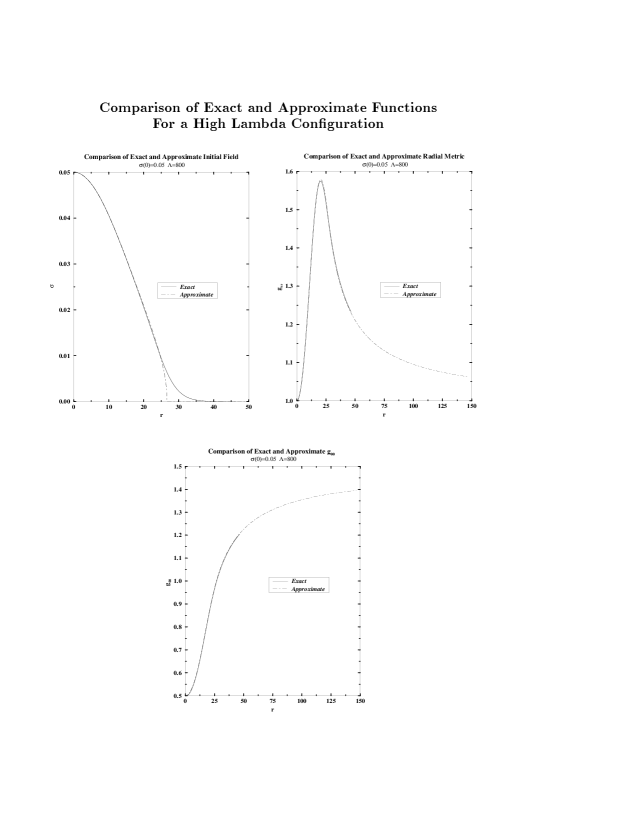
Figure 20: The equilibrium profiles of a $\Lambda=800$ star with central density $\sigma=0.05$ as derived from the high-$\Lambda$ approximate equations and the exact equations are compared. A Schwarzschild exterior is attached to the approximate solution after the field vanishes. The three plots show the field $\sigma$, $g_{rr}$, and $g_{00}$ respectively. Clearly, the approximation matches the exact solution very well.

Table 1: The ratio of the QNM frequency for $\Lambda=1600$ to the QNM frequency for a given $\Lambda$ is compared to $\Lambda^{0.5}/40$ (which is the predicted ratio for large $\Lambda$) for $\Lambda=1200$, $800$, and $1600$. As expected, the higher $\Lambda$ values match better. The initial central density is $\bar{\sigma}(0)=0.4.$

3.4 Boson Stars: Formation and Stability in BD Theory

We now describe our work on the study of boson stars in the BD theory [56]. We hope to extend this work to general Scalar–Tensor theories in the future.

The equations and set up have already been described earlier. We use the evolution code described in the GR section of this chapter to study the dynamical evolution of this system. The equilibrium configurations are described in [52]. A modified version of the equilibrium code used in GR was used to find the equilibrium configurations. We then studied the time evolution of these configurations using our evolution code.

3.4.1 Boundary Conditions

For the boundary conditions, regularity dictates that the radial metric is equal to 1 at the origin. The boson field and the BD field are both specified at the origin. The boson field goes to zero at $\infty$ and the BD field goes to a constant which is fixed during the evolution. This constant does not enter into any of the evolution equations as all the terms in the set of equations are derivatives in the BD field.

The inner boundary at the origin requires that the derivatives of the metric and all the fields vanish at this point. This is implemented by extending the range of $r$ to include some negative values. The metric components $g$, $N$, the boson field and the BD field are required to be symmetric about $r=0$. While the boson field falls off exponentially with $r$ in the asymptotic region, the BD field is more slowly varying with a $1/r$ dependence.

For the BD field, $\varphi$, the wave equation can be written as

$$\varphi(r,t)=\varphi_{\infty}+{1\over r}\,F\left(t-{r\over c}\right)$$ (81)

which is an exact condition for 1-D waves. Differentiating, one gets

$$\left.{1\over c}\,{\partial\varphi\over\partial t}+{\partial\varphi\over\partial r}+{(\varphi-\varphi_{\infty})\over r}\,\right|_{\mathchoice{\hbox{{outer edge}}}{\hbox{{outer edge}}}{\hbox{{outer edge}}}{\hbox{{outer edge}}}}=0.$$ (82)

Note that this technique used by Novak [57] in a study of stellar collapse.

For the boson field, $\Psi$, an outgoing boundary condition to order $1/r$ is

$$\beta^{2}\,k^{2}=\omega_{E}^{2}-N^{2}\,m^{2}\,e^{2a}.$$ (83)

Therefore at the outermost grid point we require that

$$\partial_{t}\partial_{t}\tilde{\Psi}=-\beta\,\partial_{t}\partial_{r}\tilde{\Psi}-\frac{N^{2}}{2}\,\tilde{\Psi}\,e^{2a},$$ (84)

where $\tilde{\Psi}=r\,\Psi$ is the field variable whose evolution equations are set up in the code.

We also use a sponge to remove second order reflections. It reduces the momentum of the boson field artificially, and is irrelevant for the massless BD field. It is a damping term that effectively simulates a potential term in the wave equation. This potential is large for incoming waves (proportional to $k+\omega_{E}$) and small for outgoing waves (proportional to $k-\omega_{E}$). Therefore, we add an additional term in the evolution equation for $\Pi_{\Psi}$ (8)

$$\frac{V(\Psi\Psi^{\dagger})}{e^{a}\,N}(\Pi_{\Psi}+\partial_{r}\tilde{\Psi})$$ (85)

for $r_{end}-D\leq r\leq r_{end}$ where $r_{end}$ is the $r$ value of the outermost grid point and $D$ is an adjustable parameter representing the width of the sponge. $D$ is typically chosen to be a few times the wavelength of the scalar radiation moving out.

The equilibrium sequences have similar profiles to GR [52] with of course the additional BD profile. The perturbations are described in the GR subsection. While the mass loss in GR must solely be due to scalar field radiation there is an additional possibility here of gravitational field radiation through oscillations of the BD field even though we have spherical symmetry.

3.4.2 Ground State Results

• $S$-branch evolutions

After confirming that our code was stable and the equilibrium profile of the star was undisturbed for several thousand time steps, we let the system evolve under infinitesimal perturbations (less than $0.1\%$ mass change from equilibrium). The system started oscillating at its fundamental quasinormal mode frequency. The BD field also acquired this oscillation frequency.

In GR, a QNM frequency increases as $\Phi_{c}$ become larger (radius become smaller) up to a point before starting to decrease rapidly to zero as it approaches the density corresponding to maximum mass signalling the onset of instability [35, 50]. We found the same feature in BD.

In addition, the system takes on the proper underlying frequency, which originates from the time dependence of the boson field $\Psi\sim e^{it}$. This frequency corresponds to period $2\pi$ in $t$ in our units, and leads to metric and BD field oscillations with period $\pi$, from the structure of the equations. To show this feature we have enhanced the BD field oscillation (Fig. 22) in Fig. 23. The time interval between the ticks on the horizontal axis is $\pi$.

Under large perturbations, a stable boson star in GR expands and contracts, losing mass at each expansion. The oscillations damp out in time and the system finally settles down into a new configuration on the $S$-branch. These features are now also observed in BD theory.

We show the effects of a large perturbation on a stable BD boson star described above. The example we present is the case of initial data with $\Phi_{c}=0.2$, mass $M=0.540G_{*}/m$ after perturbation (about $13\%$ lower in mass compared to unperturbed equilibrium configuration of $M=0.622G_{*}/m$).

The maximum radial metric $g_{rr}$ and the central BD field as a function of time are shown in Fig. 24 and Fig. 25, respectively. In both figures, we have plotted the case of $\omega_{BD}=600$, and $\omega_{BD}=60$ as well as GR. The increase of the maximum $g_{rr}$ indicates the star is contracting, reaching its maximum value at the end of the contraction in a cycle. Then, as the star expands, the maximum $g_{rr}$ decreases, reaching its minimum at the end of the expansion. These processes repeat themselves with the oscillations damping out in time as the star settles to a new stable configuration with maximum radial metric of smaller value than it started with (lower mass). The lower value of the BD parameter shows a phase shift in comparison to GR, which might be suggestive of a different rate of approach to the final configuration. We see the same dynamical behavior in the BD field (Fig. 25). It has the same oscillation frequency as that of the metric. The oscillations damp out in time and the BD field settles to a value closer to zero than it started at (lower final mass).

The system loses mass through radiation during its evolution. A comparison of the mass as a function of time for the BD case ($\omega_{BD}=600$ and $60$) as well as GR shows little difference, indicating that the radiation is mostly scalar field radiation from the boson field and not scalar gravitational radiation due to the BD field. This is despite the BD field oscillating in the BD case and being zero in the GR case.

The amount of mass radiated progressively decreases, as can be seen in the luminosity profile ($-{dM}/{dt}$ versus time) shown in Fig. 26. Here again a comparison between GR and the two BD parameters is shown. Again we see the phase shift for the lower BD parameter (further from GR). The system finally settles to a new state of smaller mass.

Figure 22:         Quasinormal mode oscillation of a stable boson star. The maximum value of the metric $g_{rr}$, and the central Brans-Dicke field $\varphi(r=0)$ are plotted as functions of time. Both of them take on the QNM frequency of the star. The oscillation is virtually undamped for a long period of time.

Figure 23: The magnification of the second figure of Fig. 22 is shown. In the dimensionless units we have adopted, the time interval between the ticks on the horizontal axis is $\pi$. We see the Brans-Dicke field oscillates with period $\pi$. Thus it has twice the frequency of the boson field, which oscillates with period $2\;\pi$.

Figure 24: Finite perturbation of an $S$-branch boson star. Maximum metric $g_{rr}$ is plotted. The metric is damped in time as the star settles to a new configuration.

Figure 25: The same model as Fig. 24. The central Brans-Dicke field $\varphi(r=0)$ is plotted. We see the oscillations damp out as the star settles down, indicating again transition to a new stable boson star configuration.

Figure 26: The same model as the previous figures. ‘Luminosity’ $L=-dM/dt$ is plotted versus time. Clearly the radiation is decreasing in time.

• Evolution of $U$-branch stars and excited stars

Boson stars on the $U$ branch and excited states are inherently unstable in GR [35, 50]. Under perturbations that reduce the mass, boson stars on the $U$ branch can migrate to the stable branch. In this section, we will see that these features also exist in BD theory. Configurations can be perturbed in such a way so as to decrease their mass enough that they migrate to new configurations on the $S$-branch. On the other hand, in GR, if they do not lose mass and migrate, then the boson stars of configurations with $M<N_{p}\,m$ collapse to black holes. Stars with $M>N_{p}\,m$ disperse and radiate out to infinity. We also see these features in BD theory.

Our first dynamical example from $U$-branch boson stars is a migration process. As in GR, we have also seen migrations of these stars to the stable branch when we remove enough scalar field smoothly from some region of the star so as to decrease the mass by about $10\%$. In particular, we show the migration of a star of central boson field $\Phi_{c}=0.35$ with unperturbed mass 0.625 $G_{*}/m$. After perturbation, its mass is reduced to 0.558 $G_{*}/m$. In Fig. 27, we show the maximum value of metric $g_{rr}$ and central value of BD field $\varphi(r=0)$ versus time. The initial sharp drops in both lines occur as the star rapidly expands and moves to the stable branch. After that it oscillates and finds a new configuration to settle into. The damping of oscillations as it settles down is clearly seen in the figure. We see also the BD field oscillations damping out as the star gets closer and closer to its final state.

The ratio of mass at time $t$ to the initial mass for BD with parameter $\omega_{BD}=60$, $600$ and the GR case is shown in Fig. 28. The flattening of the curve at later time is indicative of the star settling down to a new configuration. Although convergence towards GR with increasing $\omega_{BD}$ is clearly indicated, there is no significant difference between the three cases. The amount of total mass extraction from the system is slightly suppressed if we evolve in the BD theory. By the time of 7500 shown in the plot, we see that the mass of the star is about 0.045 $G_{\ast}/m$, which corresponds to an equilibrium configuration with $\Phi_{c}=0.06$, while our central density $\Phi_{c}$ is about 0.061, meaning that the star is quite close to its final configuration.

In contrast to the previous example, if we add a small mass to $U$-branch stars, we can see the formation of a black hole in its evolution. In Fig. 29, we plotted an example of such an evolution, suggesting formation of a black hole. The initial data of this plot is boson star of central boson field $\Phi_{c}=0.35$ (the same value with the previous migration case) and the system is perturbed very slightly so that the perturbed mass is less than $0.5\%$ greater than its initial mass. The sudden collapse of the lapse function is indicative of the imminent formation of an apparent horizon. (Due to the polar-slicing condition in our code [38] we will never see the horizon actually form). In addition to this the radial metric starts to grow rapidly and the code is no longer capable of handling the resulting sharp gradients. As an indicator of the suddenness of the process, we see that in the configuration shown the lapse has fallen to a value of about $0.003$ by a time of 60 after being at $0.230$ at a time of $55$ and $0.5$ at a time of $50$ (the latter two points are not shown in the plot).

There is almost no loss in mass in this system and the time of collapse is quite close to that in GR. In the GR case, we confirmed the formation of black hole [58] very shortly after this point ($\approx 3\,M$ where $M$ is the mass of the system) by switching this data into 3-dimensional code and evolving the system. Therefore we expect almost the same behavior in the BD case.

The black hole formation in the BD theory has been investigated by Scheel, Shapiro and Teukolsky for dust collapse [59]. They found that the dynamical behavior of the apparent horizon is quite different in the physical Brans-Dicke frame, but the same as GR in the Einstein frame. Their results therefore also support our discussion of the formation of black hole in the BD theory.

3.4.3 Excited States

Excited states of boson stars in general are not stable in GR. They form black holes if they cannot lose enough mass to go to the ground state. We confirm the same features for the BD case. In Fig. 30, we plot the metric $g_{rr}$ of dynamical transition from an excited state with 3 nodes to a ground state boson star configuration. The initial configuration has four metric maxima and the final has one. After it goes to the ground-state branch, it oscillates and compactifies to form a new configuration. We show the oscillations of the star from a time of $27300$ to $28400$ in Fig. 31. The $95\%$ mass radius at this stage is about $100$ and the star has still to reach its final state.

Figure 27: Migration of an unstable boson star to a stable configuration; central Brans-Dicke field $\varphi(r=0)$ and maximum of $g_{rr}$ is plotted. There is a sharp initial drop in the radial metric as the star moves to the stable branch. The oscillations damp out in time as the star settles down.

Figure 28: Comparisons of total mass of the system $M$ rescaled by its initial mass $M_{init}$ during a migration process from $U$-branch star. Three lines are plotted. Although the mass-loss is similar in the three cases, the curve corresponding to the higher Brans-Dicke parameter is clearly closer to GR (as it should be).

Figure 29: Dynamical transition from $U$-branch star to a black hole. The metric $g_{00}$ is plotted. The collapse of the lapse function is indicative of imminent black hole formation.

Figure 30: Dynamical transition from an excited state to a ground state boson star configuration. The metric $g_{rr}$ is plotted. The initial four peaks indicative of a three-node star cascades to the ground-state branch after a long time evolution.

Figure 31: Dynamical transition from an excited state to a ground state boson star configuration. The metric $g_{rr}$ is plotted at later times to show its oscillations after the star reaches a ground state.

3.4.4 Formation of Boson Stars

In the previous sections, we have analyzed boson stars in BD theory, starting with equilibrium or perturbed equilibrium configurations. However, we have not discussed whether or how such an equilibrium configuration actually forms from generic initial data in BD theory. In this section, we answer this question by demonstrating the formation of boson stars in BD theory. The formation of boson stars in GR has been discussed by Seidel and Suen [60], for some set of initial data of non-zero measure.

We start our evolution with initial data given by a Gaussian packet in the bosonic field $\Phi$. This represents a local accumulation of matter field:

$$\Phi=a\exp(-bx^{2}),$$ (86)

where $a$ and $b$ are free parameters. We set the BD field $\varphi$ to be flat at the initial stage, so as to see if local inhomogeneity of the matter will form a boson star in BD theory. We reintegrate the lapse equation and Hamiltonian constraint equation to provide metric functons on the initial slice. We then observe its evolution.

We find that, with particular parameters $a$ and $b$, this system forms a stable equilibrium configuration, which can be recognized as the formation of a boson star. As a demonstration, we here show an evolution with parameters $a=0.1$ and $b=0.025$. The BD parameter $\omega_{BD}$ is taken to be $600$. In Fig. 32, we show the BD field $\varphi$ as a function of radial coordinate at various earlier times of evolution. We see that the BD field becomes negative quickly and begins oscillating around a particular value. In the figure one can see that the BD field $\varphi$ between $r=40$ and $r=50$, and at around $t=50$ is still not near its final configuration. The long time evolution of BD field is shown in Fig. 33, in which we show the BD scalar field $\varphi_{BD}$ at the center for early times, intermediate times, and late times. We can see the field settling down to a periodic oscillation in final phase, similar to the migration and transition cases in the previous section. The initial mass of this configuration in units of $G_{\ast}$ is $0.39$ and the final mass (at the end of our simulation) about $0.384$. At this stage the magnitude of the central boson field is oscillating between 0.032 and 0.048. The BD field oscillates between $-0.00126$ to $-0.00166$. This range of boson oscillations corresponds to masses between 0.342 and 0.410 respectively while the BD field oscillations give a mass between 0.355 and 0.405 respectively. Given that the mass at this stage is $0.384$ (consistent with the above) we expect that the final mass will be between $0.355$ and $0.384$.

We show the luminosity $L(-{dM}/{dt})$ versus time $t$ curve in Fig. 34 during the same periods as in Fig. 33. In the early stage, we see one pulse is emitted from the system. This is related to the outgoing pulse from our initial boson field configuration. After this initial pulse, the system starts oscillating with a period $\pi$ (twice the frequency of the boson field oscillation) and the star begins forming. After that, we see the luminosity $L$ begin damped oscillations as a function of $t$. (We cut out the initial large amplitude luminosity around $t=200$). Even though the system’s evolution is followed for a long time, the accuracy of the calculation is quite good with the Hamiltonian constraint satisfied to order $10^{-7}$ or better.

We also note that certain parameters $a$ and $b$ (mentioned at the beginning of this section) will result in star formation but others will not. If we choose large amplitude $a$ and small $b$, then the initial configuration has too large a mass and is not dispersive enough resulting in black hole formation during evolution. In the opposite limit if we have a very narrow localized wave packet it has a tendency to be dispersive (as per the wave equation). So if $b$ is too large no boson star forms. Intermediate between these two are configurations that form stable stars. For example, if $a=0.1$, then at $b=0.01$ a black hole is formed, while at $b=0.025$ a boson star forms as we have shown, and at $b=0.035$ the configuration disperses away to flat space at the end of the evolution. On the other hand for $b=0.01$ and $a=0.05$ a boson star forms. This demonstrates that the boson star is a realizable object even in the BD theory, and opens windows to study them and other similar nontopological solitonic objects in astrophysical roles.

Figure 32: An example of formation of boson star in Brans-Dicke theory. Snapshots of $\varphi_{BD}(r)$ are plotted for initial stage of evolution.

Figure 33: An example of formation of boson star in Brans-Dicke theory. Dynamical behavior of the Brans-Dicke scalar field $\varphi_{BD}(x=0)$ is plotted for three evolution regions: early time, intermediate time, and late time. We can see the field settling down to an equilibrium configuration (periodic oscillation).

Figure 34: The emitted luminosity $L=-dM/dt$ is plotted as a function of time. In the first stage of evolution the luminosity data takes on an underlying oscillation of period $\pi$. The frequency of this oscillation is twice the frequency of the underlying boson field. This occurs after the emission of one Gaussian-shaped scalar pulse, related to the initial field configuration. The amount of mass loss decreases in time as the star forms and settles down.

3.5 Boson Halos

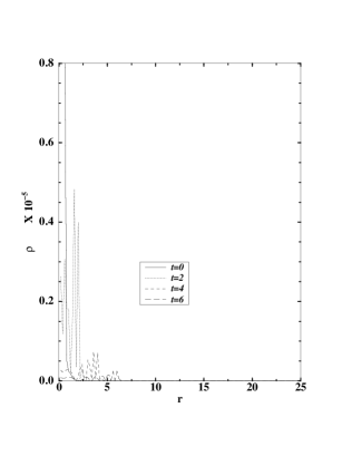
Figure 35: The inability of massless scalar field configurations to form compact self-gravitating objects as discussed by Christodoulou and others [61, 62] is verified numerically. An initial field configuration of the form $\sigma=0.001\cos(r)\exp(-r)$ is seen dispersing in the plot. The dispersal takes place very quickly.

In the last chapter we described the nature of the equilibrium configurations of Boson Halos, made of massless scalar particles. To study the formation of these objects we use the evolution equations ($BD$ evolution equations with $a=m=0$) and use the same code described in the first section of this chapter. Earlier studies, both numerical and analytical, have confirmed that self-gravitating objects with massless scalar fields cannot be compact [61, 62]. Thus taking a Gaussian type localized distribution of scalar matter and evolving the system using the evolution equations described above, results in dispersal of the scalar matter without forming any self-gravitating object. Even sinusoidal functions that were damped by exponential decays met with the same fate. These were functions like $\exp(-r)\sin(r)/r$ and $\exp(-r)\cos(r)$. In Fig. 35, a plot of the density versus the radius for different times is shown for $\sigma=0.001\cos(r)\exp(-r)$. The star dissipates very quickly. A Gaussian distribution represents a local accumulation of matter and is obviously the most likely happening. It seems though that only specialized distributions can give rise to these halos.

The initial configurations for the scalar field that yield stable configurations were those characterized by a $1/r$ times a sinusoidal dependence at large $r$ as well as an energy density $\rho$ that had points of inflection. These were typically functions like

$$\frac{\cos(r)}{1+r},$$ (87)

$$\cos(r) \left[1-\exp\left(-\frac{1}{r}\right)\right],\quad\mbox{and}$$ (88)

$$\sin(r) \left(1+\frac{1}{r}\right)\,\log\left[1+\frac{1}{1+r}\right].$$ (89)

We show the density and radial metric evolutions for a field of the form $0.003\cos(r)(1-\exp(-1/r))$. This settles into a self-gravitating object after some time. Fig. 36a shows the density as a function of $r$. The central density $\rho(0)$ increases during the evolution from its initial value at $t=0$. Fig. 36b reveals the radial metric as it evolves in time as a function of radius. This too displays the settling to a stable configuration. In Fig. 36c we show the mass loss for the system as it finds itself a configuration. The mass at fixed radial values for these times is shown in Table LABEL:mslstbl1. The amount of radiation for this system is relatively small and decreases in time.

On the other hand, functions like $1/(r+1)$ , $\cos(r)/{(1+r)}^{2}$ and $\sin(r^{1.01})/r^{1.01})$ failed to settle to a bound state and just dispersed away. Scalar fields represented by these functions did not result in $\rho$ having points of inflection.

3.5.1 Analytical Proof of Newtonian Stability

To investigate the stability of Newtonian solutions under small perturbations using the perturbative method [3, 63, 64], we write the linear scalar field perturbation in the form

$$\Phi(r,t):=\sigma(r)e^{-i\omega t}+\delta\sigma(r)e^{ik_{n}t}\;,$$ (90)

where $k_{n}$ are the frequencies of the quasinormal modes. The perturbed scalar field equation

$$\delta\sigma^{\prime\prime}+2\delta\sigma^{\prime}/x+k_{n}^{2}\delta\sigma=0\;,$$ (91)

together with the boundary conditions

$$\delta\sigma^{\prime}(0)=\delta\sigma(R)=0,$$ (92)

(for regularity of $\delta\sigma$ at the origin and at the radius $R$ of the boson halo) defines a Sturm-Liouville eigenvalue problem with real eigenvalues

$$k_{1}^{2}<k_{2}^{2}<\ldots\;.$$ (93)

Eigenfunctions of this particular differential equation (91) are

$$\delta\sigma=\frac{\sin(k_{n}x)}{x}\;,$$ (94)

where the eigenvalues are real,

$$k_{n}=n\frac{\pi}{R}\;;$$ (95)

$n$ is an integer and $R$ the radius of the solution. Thus the eigenvalues $k_{n}^{2}$ are positive. This means that all modes are stable.

3.5.2 Numerical Study of Stability

We study the evolution of dilute configurations using the same numerical code we used for studying boson stars. We show a perturbed Newtonian configuration as it settles to a new Newtonian configuration. The perturbation that is used in this case mimics an annihilation of particles. A Gaussian bump of field is removed from a part of the star near the origin. Fig. 37a is a plot of the unperturbed versus the perturbed density at $t=0$. The perturbed configuration is evolved and settles to a new configuration. The scalar radiation moves out as shown in Fig. 37b. In Fig. 37c the density profile is shown after the system settles down. The system is very clearly in a new stable configuration. In Fig. 37d the mass is plotted as a function of radius for various times. Again one can see that the mass loss is decreasing by the end of the run showing that the system is settling down to a new configuration. The mass as a function of time is presented in Table LABEL:mslstbl2 for different radii.

We have so far only been successful in evolution studies of dilute configurations. The reason for this is that denser configurations need much better resolution in order for their evolution to be studied in our code. This is coupled with the difficulty that we still need the boundary to be very far away, so that the density has significantly fallen off, for an outgoing boundary condition to work. One possibility is to match our configurations with some other kind of matter at the boundary. For example, we could have a massless scalar field configuration surrounded by a massive field configuration like a boson star. Unfortunately, while we can find such configurations with smooth mappings of the metric and field density, the scalar field itself does not match smoothly for such configurations. So far, we are using either an outgoing wave condition or exact boundary conditions where the latter one simulates a vacuum energy. Further investigation is needed before we can decide whether these non-Newtonian configurations are inherently unstable.

3.5.3 Radially Oscillating Solutions: Massive Field Case

A boson star consists of scalar massive particles, hence in the simplest model one has a potential $U=m^{2}|\Phi|^{2}$. Exponentially decreasing solutions exist for special eigenvalues of the scalar field $\omega<m$, so that the star has a finite mass. In the case of $\omega>m$, oscillating scalar field solutions can be found for all values of $\omega$. The energy density reveals minima and maxima as opposed to the points of inflection seen for the massless case. Fig. 38a shows a comparison of the density profile for the two cases. In Fig. 38b we show the mass profile and the particle number as functions of central density. The binding energy is always positive making the system unstable. Numerically we find the system to completely disperse (as it should), making these parameters unfavourable as halo models.

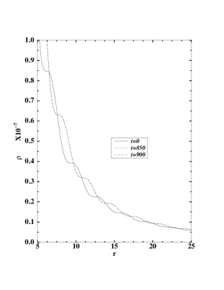
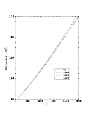
Figure 36: (a) Top left: The formation of a self-gravitating massless scalar field object is shown here for an initial field configuration of the form $0.003\cos(r)(1-\exp(-1/r))$. The density in this case increases from its initial value as the configuration settles down. (b) Top right: The radial metric for this configuration is shown evolving to a stable final configuration. (c) Bottom: The mass is plotted as a function of radius at different times. As the configuration evolves it loses less and less mass as it settles down.

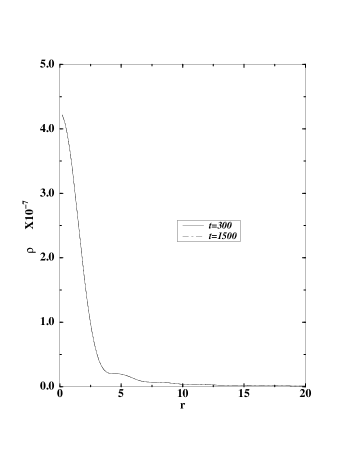
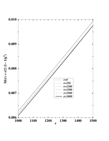
Figure 37: (a) Top left: An exact Newtonian configuration is perturbed and evolved using the GR code. The initial unperturbed and perturbed densities are shown. A Gaussian profile of scalar field is removed from the equilibrium configuration, and the constraint equations are reintegrated to give new metrics before beginning evolution. (b) Top right: The outgoing scalar radiation can be seen in a plot of the density at early times. (c) Bottom left: The density profile is shown after it starts to settle down. Between times of 300 and 1500 very little has changed in the density profile. (d) Bottom right: The mass is plotted as a function of radius for different times. In order to enhance the features only a small part of the radial region is shown. The amount of mass loss is clearly lessening in time.

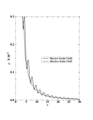
Figure 38: (a) Left: The density profiles of massive scalar field configurations with $\omega>m$ is compared to that of a massless field. The former has maxima and minima while the latter has points of inflection. This structure may be related to stability issues. (b) Right: The mass and particle number are plotted against the central density for boson star oscillators. We find in all cases that the mass is always greater than the particle number explaining their instability against a collective dispersion.

Table 2: Mass values at different radii and different times for the evolution in Fig. 36. One recognizes that the change in the mass at fixed radius decreases in time, showing that the system is settling down to a stable configuration.

	$t=0$	$t=500$	$t=700$	$t=900$
$r=800$	$0.03589375$	$0.0350625$	$0.0346250$	$0.034234375$
$r=1200$	$0.05750000$	$0.0563125$	$0.0556250$	$0.055062500$
$r=1600$	$0.08018750$	$0.0786250$	$0.0776875$	$0.076937500$

Table 3: Mass values at different radii and different times for the evolution in Fig. 37. One recognizes that the change in the mass at fixed radius decreases, hence it proves the settling to a stable configuration.

	$t=0$	$t=1500$	$t=2500$	$t=3400$
$r=500$	$0.00284700$	$0.00278000$	$0.00268750$	$0.00268375$
$r=1000$	$0.00628625$	$0.00619375$	$0.00608495$	$0.00608335$

Chapter 4 Boson Stars in $3D$ Numerical Relativity

We now describe our work on Boson stars in $3D$. One of the major drawbacks in going from a $1D$ code to a $3D$ code was the paucity of grid points. Computer memory and time constraints limited grid resolution. There was no simple outgoing wave condition (the boundary was no longer one point) and there was no reasonable way to implement a sponge. A sponge, while it prevents reflections, also uses up grid points. Besides, the length of the sponge had to be of the order of the wavelength of the outgoing radiation. Gravitational waves have longer wavelengths than scalar waves and this further inhibited the use of a sponge in a $3D$ code.

The $3D$ code that had been developed to deal with vacuum spacetimes was extended to include matter terms. We used our model to test the code by comparing with established results in $1D$, as well as to results of $3D$ perturbation studies. Once stability was achieved, we then used the code itself to get physical results of Boson stars under nonspherical perturbations. The main advantage with Boson stars as the matter source was that there were ordinarily no spacetime singularities as in black hole evolutions, as well as none of the surface problems that people dealing with neutron star configurations have to routinely face. The Boson field exponentially decays to zero at spatial $\infty$. Nevertheless, the small amount of matter in the outer regions that prevents surface problems could, for the purposes of wave extraction, be perfectly well regarded as a vacuum. The code used a leapfrog scheme with the extrinsic curvature (related to the time derivative of the metric) and time derivatives of the Boson field on half integral time steps ($n+1/2$) while metric fields and Boson fields were on the integral timesteps ($n$). To prevent grid point to grid point instabilities due to mesh drifting we routinely used a small amount of diffusion in the center of the star, as described in the last section of the introduction of this thesis.

In an appendix we describe how we scaled the variables in our $3D$ code. This appendix shows how to relate a unit of computer time to physical time in terms of the mass of the configurations.

4.1 Stress Energy Tensor, Energy Density, Momentum Density, Sources

The metric components in the $ADM$ formalism are given in (182) and (183). The lapse is $N$ and the shift components are $N^{i}$. In the introduction to the thesis we wrote down the matter Lagrangian for a Boson star in scalar-tensor theory and showed how to get the stress-energy tensor from it. In $GR$ we get the equations with the parameter $a$ set to zero. The stress-energy tensor is then

$$T_{\mu\nu}={\psi_{1}}_{,\mu}\,{\psi_{1}}_{,\nu}-\frac{1}{2}\,g_{\mu\nu}\,[{\psi_{1}}_{,\alpha}\,{\psi_{1}}^{,\alpha}+m^{2}\,{\psi_{1}}^{2}]+({\psi_{1}}\rightarrow{\psi_{2}}).$$ (1)

where the subscripts $1$ and $2$ refer to the two real components of the complex Boson field. Since we rescale quantities to dimensionless ones no factor of $m$ finally appears in the Einstein equations. (An appendix attached to this thesis explains the scaling in the $3D$ code). Thus we can write

$$T_{\mu\nu}={\psi_{1}}_{,\mu}\,{\psi_{1}}_{,\nu} - \frac{1}{2}\,g_{\mu\nu}\Bigg{[}$$ (3)

$$g^{00}\,(\partial_{t}{\psi_{1}})^{2}+{\psi_{1}}_{x}\,(g^{xx}\,{\psi_{1}}_{x}+g^{xy}\,{\psi_{1}}_{y}+g^{xz}\,{\psi_{1}}_{z})$$

$$+ {\psi_{1}}_{y}\,(g^{yy}\,{\psi_{1}}_{y}+g^{xy}\,{\psi_{1}}_{x}+g^{yz}\,{\psi_{1}}_{z})$$ (4)

$$+ {\psi_{1}}_{z}\,(g^{zz}\,{\psi_{1}}_{z}+g^{zy}\,{\psi_{1}}_{y}+g^{xz}\,{\psi_{1}}_{x})+{\psi_{1}}^{2}\Bigg{]}$$ (6)

$$+({\psi_{1}}\rightarrow{\psi_{2}}).$$

Here the subscripts $x$, $y$, and $z$ refer to a partial derivatives with respect to those variables. The form of the density is given by $n^{\mu}n^{\nu}T_{\mu\nu}$ where $n^{0}=1/N$ and $n^{i}=-N^{i}/N$. Thus

$$\rho=\frac{1}{N^{2}}\,T_{00}-\frac{N^{i}}{N^{2}}\,T_{0i}+2\,\frac{N^{i}N^{j}}{N^{2}}\,T_{ij}.$$ (7)

The scalar field equation is the gravitational Klein–Gordon equation:

$$0 = {\vbox{\hrule height=0.5pt\hbox{\vrule width=0.5pt,height=8.0pt\kern 8.0pt\vrule width=0.5pt} \hrule height=0.5pt}}\psi-\psi=(g^{\alpha\beta}\,\psi_{,\beta})_{;\alpha}-\psi$$ (8)

$$= \psi^{,\alpha}{}_{,\alpha}+\Gamma^{\alpha}{}_{\alpha\beta}\,\psi^{,\beta}-\psi$$ (9)

$$= \psi^{,\alpha}{}_{,\alpha}+\frac{1}{2}\,g^{\alpha\nu}\,g_{\nu\alpha,\beta}\,\psi^{,\beta}-\psi$$ (10)

$$= \psi^{,\alpha}{}_{,\alpha}+\frac{1}{\sqrt{-g}}\,(\sqrt{-g})_{,\beta}\psi^{,\beta}-\psi$$ (11)

$$= \frac{1}{\sqrt{-g}}(\sqrt{-g}\,\psi^{,\alpha})_{,\alpha}-\psi.$$ (12)

where the factor $g$ represents the determinant of the 4 metric. Thus

$$\frac{1}{\sqrt{(N^{2}-N^{i}\,N_{i})}\,\sqrt{\gamma}}\,\left(\sqrt{(N^{2}-N^{i}\,N_{i})}\,\sqrt{\gamma}\,g^{\alpha\beta}\,\psi_{,\beta}\right)_{,\alpha}-\psi=0.$$ (13)

These second order (in time) equations ($\alpha=\beta=t$) can be conveniently converted to first order by defining a new variable $\pi=\sqrt{(N^{2}-N^{i}\,N_{i})}\,(\sqrt{\gamma}\,g^{tt}\,\dot{\psi})$ or, since we have two fields

$$\pi_{a}=\frac{\sqrt{(N^{2}-N^{i}\,N_{i})}}{N^{2}}\left(\sqrt{\gamma}\,\dot{\psi_{a}}\right)\quad a=1,2.$$ (14)

This gives the evolution of $\pi$ to be of the form

$$\dot{\pi}= - \sqrt{(N^{2}-N^{i}\,N_{i})}\,\sqrt{\gamma}\,\psi$$ (15)

$$+ \partial_{i}\left({N^{i}}\,\pi\right)+\partial_{t}\left(\sqrt{(N^{2}-N^{i}\,N_{i})}\,\sqrt{\gamma}\,\frac{N^{i}}{N^{2}}\,\partial_{i}{\psi}\right)$$ (16)

$$+ \partial_{i}\left(\sqrt{(N^{2}-N^{i}\,N_{i})}\,\sqrt{\gamma}\,\gamma^{ij}\,\partial_{j}\psi\right).$$ (17)

4.2 Testing the Scalar Evolver

We computed the derivatives of the fluxes $\gamma^{ij}\sqrt{(N^{2}-N^{i}N_{i})}\sqrt{\gamma}$ using a second-order scheme. We also adopted a second-order scheme for the first and second-order derivatives $\partial_{i}\psi_{a}$ and $\partial_{j}\psi_{a}$. (The subscript $a$ runs from $1$ to $2$ representing the two real components of the boson field). We used a staggered grid (the origin was not one of the points). In order to be better able to resolve the star we observed evolutions on an octant rather than the full grid so our perturbations also had to retain this octant symmetry. The first grid point was actually staggered half a spacing step away from the origin in one direction and the second grid point was half a step in the other direction.

The first stage of the analysis was to get initial data. Spherically symmetric equilibrium data was obtained from the $1D$ code, described in the last chapter. This data was then interpolated onto a $3D$ grid. This was done by identifying the positions $r(i,j,k)$ on the $3D$ grid, finding out which point it was closest to on the $1D$ grid, and using the $1D$ data before that point, at that point and the point after that, to get the value at $r(i,j,k)$ with a three-point interpolator. This $3D$ data for the boson fields and for the metrics was then converted from $r,\theta,\phi$ coordinates to $x,y,z$ using

$$x^{2} + y^{2}+z^{2}=r^{2},$$ (18)

$$x = r\,\sin\theta\,\cos\phi,$$ (19)

$$y = r\,\sin\theta\,\sin\phi$$ (20)

$$z = r\cos\theta,\,\,\mathchoice{\hbox{{and}}}{\hbox{{and}}}{\hbox{{and}}}{\hbox{{and}}}$$ (21)

$$g_{ij} = \frac{\partial i^{\prime}}{\partial i}\frac{\partial j^{\prime}}{\partial j}g_{i^{\prime}j^{\prime}},$$ (22)

where the $i$ and $j$ coordinates refer to $x,y,z$ and the prime coordinates to $r,\,\theta,\,\phi$.

To test the scalar evolver we then froze the metric evolution and just allowed scalar field evolutions. (This is physically reasonable since an equilibrium boson star is characterized by a static metric.) When, after thousands of time steps, the boson field continued oscillating with a period of $2\pi$ (since the boson fields have time dependence of the form $\cos(t_{code})$ and $\sin(t_{code})$ where $t_{code}=\omega_{E}t$), we were convinced that our scalar evolver was doing well.

The boundary conditions used were reflection symmetry at the origin and flat boundary conditions for the fields at the outer boundary. We present a plot of the scalar evolver in Fig. 1.

Figure 1: A plot of the density $\rho$ as a function of $r$ until a time $t=1000$ for a boson star of central field density $\sigma=0.05$ (mass $0.416\,M_{Pl}^{2}/m$), without any metric evolution. The drift in density is insignificant over this time showing the scalar evolver to be functioning well. (That is: all the curves lie on top of each other and cannot be visually distinguished.)

When calculating $(f\psi^{\prime})^{\prime}$ (where $f$ is the flux and $\psi$ is the boson field) in the evolution of $\pi$ (equation (15)), it was numerically more advantageous to first write

$$(f\,\psi^{\prime})^{\prime}=f\,\psi^{\prime\prime}+f^{\prime}\,\psi^{\prime},$$ (23)

and then to calculate the two terms on the RHS separately. This avoids the numerical instabilities typically generated by finite differencing a finite difference.

4.3 Equilibrium Boson Star

The first step in testing the efficacy of the code was to take the known results of the $1D$ code and reproduce them in the full $GR$ code. Once the scalar evolver was found to be producing accurate results we wanted to test the code with full metric evolutions. Initially, we used equilibrium data obtained from our $1D$ spherical code.

The equations for full evolution have been developed in the introductory part of this thesis (1.3.5). The four gauge degrees of freedom were used to set the three shift components to zero and then a maximal slicing condition was used for the lapse.

4.3.1 Maximal Slicing

The condition for maximal slicing [36, 65] is $TrK=0$. Thus, on replacing for ${}^{3}R$, from the Hamiltonian constraint equation (202) (with $K=0$), into (207), we get

$$\frac{dTr\,K}{dt}=0=-N^{|i}{}_{|i}+N\left[K_{ij}K^{ij}+4\,\pi(\rho+Tr\,S)\right].$$ (24)

Here $S=S^{i}_{i}$ where $S_{ij}=T_{ij}$. The reason for writing it in this form was due to the presence of second derivatives in the Ricci tensor. The code had originally been developed for black hole spacetimes. Late time peak development in the metric functions rendered computation of second derivatives difficult. The above form was therefore numerically more advantageous [66]. This was important in the boson star collapse problem as well.

One of the advantages of the maximal slicing condition was that it provided a linear equation for the lapse. The disadvantage was that an elliptic equation had to be solved on each time slice. Asymptotic flatness required the lapse to go to some constant in the limit $r\rightarrow\infty$. In our code the value of this constant was influenced by the underlying frequency of the scalar field and the lapse value at $\infty$ was the value of that frequency (see chapter 2).

The main advantage of maximal slicing was its singularity avoiding ability. One of the advantages of a good coordinate system is avoidance of physical singularities by slowing down of evolution in the spatial region near such a singularity. The maximal lapse collapsed, vanishing exponentially, near the singularity and froze the evolution there (near $r=0$, the physical singularity for a Schwarzschild blackhole or for a Kerr metric), allowing the maximal slices to span the rest of the future development of the initial data. This was important in the boson star collapse problem. Coordinate volumes usually shrink in the neighborhood of singularities. This is avoided by maximal slicing since the $TrK=0$ condition translates in the zero shift case to the volume $\sim\gamma$ being constant. Another advantage of the maximal slicing condition is that asymptotically it turns to a natural radiation gauge in which the gravitational radiation has a wavelike propagation.

4.3.2 The Elliptic Solver

In equation (24) there is a term of the form ${}^{3}{\vbox{\hrule height=0.5pt\hbox{\vrule width=0.5pt,height=8.0pt\kern 8.0pt\vrule width=0.5pt} \hrule height=0.5pt}}N$ and, as we did for the Klein–Gordon case (8), we write the maximal slicing lapse equation:

$$\partial_{i}(\sqrt{\gamma}\,\gamma^{ij}\,\partial_{j}N)=N\,\sqrt{\gamma}\,\left(K^{ij}\,K_{ij}+4\,\pi\,(\rho+S)\right)$$ (25)

The code used a conjugate matrix solver developed at the $NCSA$ to which we added the matter terms. The basic technique was to first finite difference the above equation to second order. Because we were not dealing with flat space there were mixed derivative operators $\partial_{i}\partial_{j}$ with $i\neq j$ as well. Thus the second order finite differencing did not just connect points ($i+1,j,k$), ($i,j,k$), ($i-1,j,k$), ($i,j+1,k$), ($i,j-1,k$), ($i,j,k+1$), and ($i,j,k-1$), a seven-point stencil. It also connected 12 more points ($i+1,j\pm 1,k$), ($i-1,j\pm 1,k$), ($i+1,j,k\pm 1$), ($i-1,j,k\pm 1$), ($i,j+1,k\pm 1$), and ($i,j-1,k\pm 1$) where $i$ $j$ and $k$ are the $x$, $y$ and $z$ coordinate positions respectively. Thus we were dealing with a 19-point stencil. For ease of visualization we show the $2D$ case in Fig. 2 and the $3D$ case in Fig. 3. (In $2D$ we have a five-point stencil when there are no mixed derivatives and a nine-point stencil when mixed derivatives are present.)

Figure 2: a) Top: The five-point stencil in $2D$ in flat space is shown. The absence of mixed second-order derivatives in the $x$ and $y$ directions ensures that no points along the diagonal (except the center) are required. b) Bottom: In curved space the second-order derivatives include mixed derivatives ($\frac{\partial^{2}}{\partial x\partial y}$). We now have a nine-point stencil that includes the corner points.

Figure 3: a) Top: An extension of the previous figure to $3D$ is shown. The first figure shows a seven-point stencil, for the second-order derivatives in flat space. b) Bottom: In curved space the second-order derivatives include mixed derivatives ($\frac{\partial^{2}}{\partial x\partial y}$, $\frac{\partial^{2}}{\partial x\partial z}$, and $\frac{\partial^{2}}{\partial x\partial z}$, and their permutations). We now have a 19-point stencil.

This gave an algebraic equation of the form

$$\sum_{p,q,r=-1}^{p,q,r=+1}C_{i,j,k}^{p,q,r}\,N_{i+p,j+q,k+r}=0$$ (26)

where the sum was over non-repeating terms and had 19 coefficients $C$. It had to be solved at each grid zone except boundaries,

The conjugate gradient method involves solving the problem by solving an analogous minimization problem. Consider a set of difference equations

$${\bf A}f=b$$ (27)

where $f$ is the vector of unknowns (here our lapse value at each grid zone) and ${\bf A}$ is an $N_{g}\times N_{g}$ square matrix ($N_{g}=$ number of grid zones) containing the finite differenced coefficients at each grid zone. The right hand side is a vector of source terms.

Define the quadratic function

$$V(f)=\frac{1}{2}\,f^{{\dagger}}\,{\bf A}\,f-b^{{\dagger}}\,f.$$ (28)

Therefore

$$\frac{\partial V}{\partial f}={\bf A}\,f-b={\bf r}.$$ (29)

Thus solving (27) is the same problem as minimizing the potential $V$. Note that $A$ is the matrix

$$A_{ij}=\frac{\partial^{2}\,V}{\partial f_{i}\partial f_{j}},$$ (30)

which is symmetric. So to apply this method the finite difference equations have to be written in symmetric form.

The minimization of the potential function is carried out by generating a succession of search directions ${\bf s}$, with improved minimizers $f_{i}$ at each stage. In a maximum of $N_{g}$ iterations a solution is found.

However since we have a 19-point and not an $N_{g}$-point stencil, a lot of the matrix elements will be zero. (The matrix $A$ is a sparse matrix.) Since the finite difference equations connect points immediately to either side of a a given point, as one steps up the grid from point to point, there is a definite structure to system. The matrix has a banded diagonal structure with each diagonal band corresponding to one of the 19 finite differenced coefficients. The coefficients are stored as 19 three-dimensional arrays, meaning $19N_{g}$ not $N_{g}^{2}$ total elements. This reduces the number of steps needed to minimize the function. For details see [51, 66].

4.3.3 Results of Maximal Slicing for Equilibrium Boson Stars

With the above machinery in place we ran the code with maximal slicing. Our grid resolution was $dx=dy=dz=0.35$ and the grid dimension was $96\times 96\times 96$. The outer boundary condition on the boson fields was flat (equal to the neighbor) and that on the metrics was static. In Fig. 4 we show a plot of the radial metric as a function of radius at various times. Clearly, this metric was not the static metric expected of an equilibrium star.

Figure 4: Radial metric drift, with maximal slicing, for an equilibrium boson star of central field density $0.05$.

The reason for this was a lack of gauge control. This is clear from the metric function $g_{\theta\theta}$ which should really be $r^{2}$ in a perfectly spherically symmetric run. For ease of visualization we plot $g_{\theta\theta}/r^{2}$ as a function of $r$ at various times and observe its drift from unity. This is shown in Fig. 5.

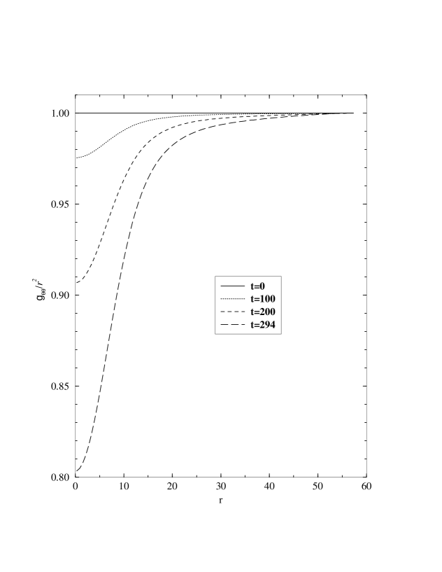
Figure 5: The drift of $g_{\theta\theta}/r^{2}$ from unity is shown, as an indicator of loss of gauge control, for a spherically symmetric equilibrium boson star configuration.

Attempts to regain gauge control are described in the next two subsections.

4.3.4 Role of the Shift Vector

As we saw in the description of $ADM$ in the introduction, we can write $t^{\mu}$ as a sum of two terms, one along the normal to the hypersurface and the other the shift along the hypersurface. So far we have been using normal coordinates with shift vector equal to zero. Although this was the simplest choice of shift, with this choice, we have squandered our ability to implement gauge control by making specific choices of shift. From the plots of $g_{\theta\theta}$ it is clear that there is coordinate motion ($dr/dt$) due to numerical error. Maybe setting the shift terms to zero as we have done left too much residual spatial coordinate freedom? Might a shift term control this? The question now is how to choose a shift. To start with, the obvious choice seemed to be one that satisfied

$$\frac{d\,g_{\theta\theta}}{dt}=0.$$ (31)

For simplicity we used a spherically symmetric form, with

$$K_{\theta\theta} = \frac{1}{2\,N}\left(\frac{d\,g_{\theta\theta}}{dt}-2\,\Gamma^{i}{}_{\theta\theta}\,N_{i}\right)$$ (32)

$$= \frac{1}{2\,N}\left(\frac{d\,g_{\theta\theta}}{dt}+g^{rr}\,g_{\theta\theta,r}\,N_{r}\right).$$ (33)

This yields, using the $\frac{d\,g_{\theta\theta}}{dt}=0$ condition,

$$N^{r}=\frac{2\,N\,K_{\theta\theta}}{\frac{d}{dr}g_{\theta\theta}}.$$ (34)

Typically this shift was phased in over a period of time. That is, a fractional amount of the calculated value of the shift was used in the code. The fractional amount was gradually increased from 0 to 1. To circumvent dealing with boundary problems we isolated the points along the diagonal $N^{r}(i,i,i)$ into a $1D$ array. We interpolated points to fill in values of $r$ along this $1D$ array that corresponded to the $3D$ grid spacing (grid spacing along diagonal $=\sqrt{3}$ grid spacing along $x$ direction if the $x$, $y$ and $z$ directions have the same number of points). This was then extrapolated onto the $3D$ grid. This meant we needed only one boundary condition instead of worrying about all the boundary points on a $3D$ grid. Under our assumption of $N^{\theta}=N^{\phi}=0$ then,

$$N^{x}=N^{r}\,\frac{x}{r},\quad N^{y}=N^{r}\,\frac{y}{r}\quad\mathchoice{\hbox{{and}}}{\hbox{{and}}}{\hbox{{and}}}{\hbox{{and}}}\quad N^{z}=N^{r}\,\frac{z}{r}.$$ (35)

For the boundary condition we phased out the shift over the last 5 points ($N^{r}(nx-4)=0.8\,N^{r}(nx-5)$, $N^{r}(nx-3)=0.6\,N^{r}(nx-5)$ and so on till $N^{r}(nx)=0$). Although the shift rose to a peak near the center of the star, where $g_{\theta\theta}$ had drifted the most before, and did have the intended effect of lowering the metric drift, it had a wavelike structure outside the star. The wave moved out and on reaching the boundary invalidated the code. A scheme of redefining the shift in the region where it first crossed the axis was tried. We used an exponentially damped attachment of the form $N^{r}=A\,exp(-b\,r)$, with A and b determined at each time step by matching the actual shifts at points close to where it crossed the axis with this expression. This and other variations on the functional form of the exponentially phased-out shift, lent a little additional stability to the metric but the metric eventually developed a peak at the patching region of the shift and invalidated the code. Nevertheless, $g_{\theta\theta}$ was fairly well locked in place and so it was at least certain that the drift had been due to coordinates drifting.

A kicking scheme was also tried. The shift was fully phased in using the condition that best suited us at that point. A shift of the form $ae^{-br}$, matched just before where the first shift peak crossed zero, was attached from the matching point onwards. After fully phasing in this shift, one discarded this method and tried to keep $g_{\theta\theta}$ locked at its value at full phase in, by taking a snapshot of it at that time and then measuring the deviation from that value at each subsequent time step. The new shift at a given time at any point was either increased or decreased from its phased in value depending on whether $g_{\theta\theta}$ decreased or increased from its phased in value at that point. Since $g_{\theta\theta}\sim r^{2}$ therefore $\frac{d}{dr}g_{\theta\theta}\sim 2r$. Thus coordinate drift could be controlled by a shift of the form:

$$N^{r}(t) = N^{r}(t_{p})+c\,\frac{dr}{dt}$$ (36)

$$= N^{r}(t_{p})+\frac{c}{2\,r}\,\frac{dg_{\theta\theta}}{dt},$$ (37)

where $t_{p}$ was the phase in time and $c$ could be positive or negative depending on which direction the drift was heading. In principle $|c|$ was unity, but in practice it tended to be a less and one had to tune this parameter. This kicking scheme had previously been used to lock the horizon in the black hole codes [67].

Although we found definite coordinate control with these methods the code always became unstable at the outer boundary. We present comparisons of the radial metric function in simulations with maximal slicing with and without shift in Fig. 6. In Fig. 7 we present a comparison of $g_{\theta\theta}$ with and without a shift phased in. Clearly the code was more stable with the shift phased in. Unfortunately the code ran longer without a shift.

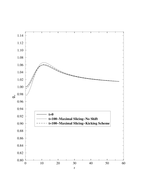
Figure 6: The radial metric function, showing markedly more drift at the same time under conditions of no shift, compared to a $g_{\theta\theta}$ freezing shift with a kicking scheme.

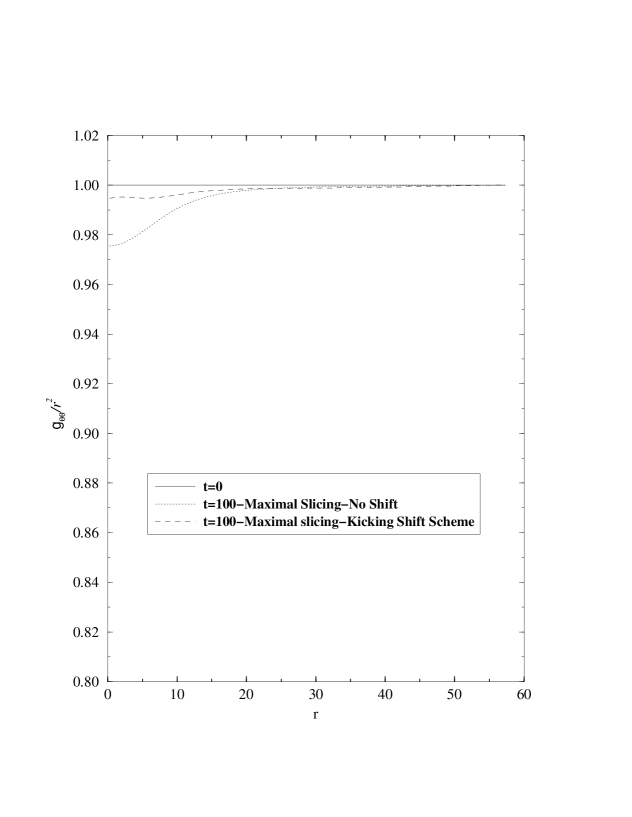
Figure 7: A plot of $g_{\theta\theta}$ shows markedly more drift at the same time under conditions of no shift compared to a shift with a kicking scheme. Both are with maximal slicing.

Even hybrid schemes were tried, with kicking done only in the outer region and the inner shift peak, that worked so well to lock $g_{\theta\theta}$, retained. This led to grid point to grid point instabilities that diffusion could not cure.

4.3.5 The K–Driver

With the shift schemes providing some control, but not to the degree that was needed, it was timely that at this time the $K$–driver was discovered. We were able to modify the $K$–driver for the boson star problem [68].

The whole point was that we needed long term gauge control, and we had been using coordinate conditions that had been tried in numerical relativity for the study of black hole evolutions. The coordinate conditions themselves were becoming unstable due to the accumulation of numerical errors during long evolutions. Shift vectors, which shifted coordinate points so they did not move normal to the constant time hypersurfaces, and time slicing conditions determining the normal direction of motion of grid points, were gauge freedoms satisfying equations that were themselves subject to numerical inconsistencies.

Consider the maximal slicing condition $K=\frac{\partial K}{\partial t}=0$ providing the elliptic equation for the lapse (24). Any perturbation (numerical roundoff) in the lapse that made $K$ nonzero, could not be forced by the slicing condition to get $K$ back to zero. The lapse might evolve to its preferred value but errors made during its perturbation at some time in the past could still create errors in the slicing condition. The initial perturbation errors in the lapse might have been caused by numerical inaccuracies like errors due to finite differencing of nonlinear equations, with low resolution. The condition

$$\frac{\partial K}{\partial t}=0,$$ (38)

written with $K=0$ could evolve to something where $K\neq 0$. Instead one considered a “K-driver” slicing condition

$$\frac{\partial K}{\partial t}+c\,K=0,$$ (39)

which without $K$ set to zero was

$$c\,K=N^{|i}{}_{|i}-N\,\left[K_{ij}\,K^{ij}-4\,\pi\,(\rho+Tr\,S)\right]-N^{i}\,K_{,i}.$$ (40)

While (24) did not actively enforce the $K=0$ condition the above slicing condition drove $K$ to zero when it was perturbed away from it. The idea being that $K\sim e^{-ct}$ exponentially went to zero, in the long run, for a positive $c$. One now could control the stability of the code by fiddling with the value of $c$ that worked best.

Finally, we actually used the K-driver for the boson star with shift equal to zero to get our best results. We needed a parameter $c=2$ near the center (typically about a third of the grid) and then we let it smoothly damp away ($ce^{-\frac{1}{3}(r-R/3)}$ with $R=r(nx,ny,nz)$ for all values of $r>R/3$). This damping factor was needed to prevent boundary problems from arising in the code. Since the drift was typically observed where the star was concentrated, this condition worked very well. We present a comparison of the zero shift maximal slicing versus the zero shift K-driver in Fig. 8.

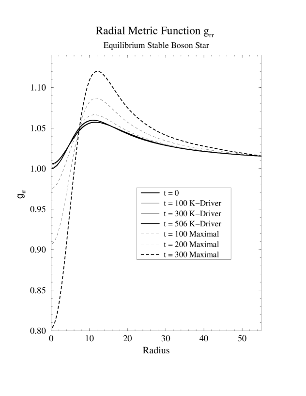
Figure 8: A comparison of the metric function drift in the time evolution of an equilibrium boson star with maximal slicing and K–driving condition is shown. The latter is clearly capable of controlling metric drift.

4.4 Spherically Symmetric Perturbations of a Boson Star.

Once the $3D$ code had been stabilized to correctly display the true evolutions of an equilibrium boson star, we went to the next step of our code tests. This was to take a boson star and observe how the code displayed its evolutions under spherical perturbations. A well tested 1-D code provided us with initial data. The initial data was time symmetric and the momentum constraints were satisfied by ensuring that the perturbation kept $\psi_{1}=\dot{\psi}_{2}$ and $\psi_{2}=-\dot{\psi}_{1}=0$ for the two boson fields. We show an oscillation of the radial metric in figures 9 and 10 (the former showing the downward part of the oscillation and the latter the upward part of it) of a boson star of original mass $0.5916\,M_{Pl}^{2}/m$ which has been reduced by about $10\%$ after perturbation.

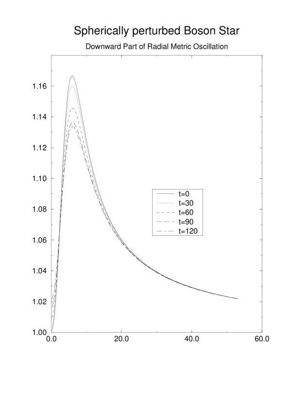
Figure 9: We show the downward part of the radial metric oscillation of a boson star that has been perturbed by a spherically symmetric perturbation. As the star expands the radial metric descends.

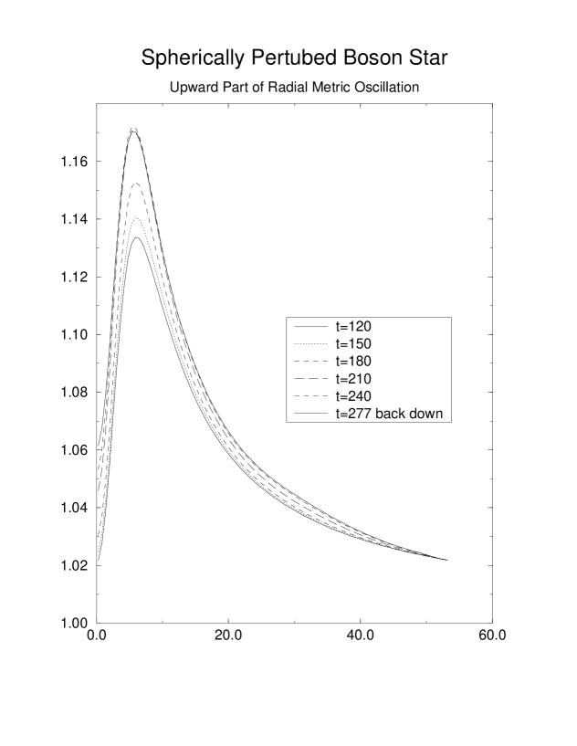
Figure 10: As the star starts to contract after its expansion in reaction to the perturbation, its radial metric starts to rise again. This part of its motion is shown in the figure. At the last step we start to see it reverse its motion again. The central field density of this star is $\psi_{1}(0)=0.15$ in the dimensionless units discussed in chapter 2. Its mass is $0.5916\,M_{Pl}^{2}/m$.

A successful code test we performed was in calculating the mass loss of a boson star under spherical perturbations and comparing it to the results we had in $1D$. In the 1-D code we calculated the mass of the star using the $ADM$ mass. Just before the sponge region (see chapter 2) we calculated the mass of the star from the radial metric

$$M=\frac{r}{2}\,\left(1-\frac{1}{g_{rr}}\right).$$ (41)

We could do this because in this region the field was small enough for the spacetime to be considered to be Schwarzschild. This was obviously not a good formula for the $3D$ code with static outer boundary conditions. We needed a more global measure of the mass so that dominant contributions from the interior of the star would not be affected by outer boundary errors. In order to calculate the mass loss we used the fact that $T^{tr}$ represents the energy flux ($ergs/cm^{2}sec$) in the radial direction. Thus integrating $T^{tr}$ over time and elemental area provided a measure of the mass loss at a given time due to scalar radiation. We calculated the mass loss in the $1D$ code by using the $ADM$ mass formula as well as integrated $T^{tr}$ and compared the results to the $3D$ case. We ran the $1D$ code with the same resolution as the $3D$ code and put detectors at the same position. We found very good agreement in all cases with different detectors and different types of perturbations. We show two plots, one with a localized spherical perturbation and the other with a global spherical perturbation, in Fig. 11 and Fig. 12 respectively. The latter plot also demonstrates the effect of resolution on the matching of the energy of scalar radiation.

Figure 11: The mass loss in $1D$ computed using the $ADM$ mass formula, and integrated energy flux $T^{tr}$, is plotted along with the integrated energy flux $T^{tr}$ using the $3D$ code for a local spherical perturbation. The closeness of values is remarkable until the effects of boundary reflections starts affecting the accuracy of the $3D$ code.

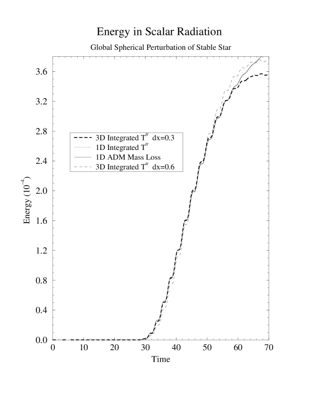
Figure 12: The mass loss in $1D$ computed using the $ADM$ mass formula, and integrated energy flux $T^{tr}$, is plotted along with the integrated energy flux $T^{tr}$ using the $3D$ code for a global spherical perturbation. The closeness of values is remarkable until the effects of boundary reflections starts affecting the accuracy of the $3D$ code. In addition the effect of grid resolution is shown by also plotting a lower resolution $3D$ calculation which shows greater discrepancy from the $1D$ result but which is still quite good.

This was indeed the key code test that showed that the code was performing well given the computational resources available.

4.5 Non-Spherical Perturbations of a Boson Star

Finally we were ready to study the behavior of boson stars under nonspherical perturbations. In the Introduction to this thesis we have already stated how Einstein’s equations under nonspherical perturbations can give rise to a wave equation. These gravitational waves, along with the scalar radiation due to our scalar field, are the two big signatures of the boson star. We have seen in the Introduction, that the Zerilli functions, Newman–Penrose Spin Coefficient $\Psi_{4}$ and the Bel–Robinson vector can provide information about the nature of this radiation and the gravitational waveform. One concern was of course whether one could extract the full waveform since the outer boundary effects could cause inaccuracies after a fairly short time as indicated by the results of the last subsection. Since the waveform extractions had to take place in the outer region of the star, which could effectively be regarded as a vacuum region, reflections from the boundary would cause problems earlier than if our detectors were placed well within the star. Here was another advantage to dealing with a boson star. As discussed in the introduction of this thesis (1.3.3), in [33] it was actually shown that the normal modes of boson stars damp out on a short time scale. The short time scale allowed us to measure all of the gravitational wave signal that contributes significantly to the gravitational energy output.

We used a grid with one octant, making sure our perturbations were axisymmetric. We used an equilibrium configuration determined from the $1D$ code and imposed on it such a perturbation. These were typically weak perturbations. Now the constraint equations had to be solved on the initial time slice in order to provide consistent fields and metric components. This was done using an initial value solver that used a relaxation method to solve the elliptic equation.

• Basics of the Initial Solver

We used the initial solver to provide new metric components by solving the Hamiltonian constraint equation (202) on the initial time slice. York’s procedure was followed [36]. We specified the initial scalar field configuration and an initial guess for the three-metric. The idea was to solve for a conformal factor $\phi$ so as to get the real metric from the guess through the relation

$$\gamma_{ij}=\phi^{4}\tilde{\gamma}_{ij}$$ (42)

where the trial metric was $\tilde{\gamma}_{ij}$. Assuming time-symmetric data, $K_{ij}=0$, the Hamiltonian constraint equation takes the form

$$R=16\pi\rho.$$ (43)

With the updated metrics (in terms of the guess and the conformal transformation) we could calculate the connection coefficients in terms of those corresponding to the guess and also get the Ricci scalar in terms of the guess

$$R=\tilde{R}\phi^{-4}-8\phi^{-5}{\tilde{\partial}_{i}}{\tilde{\partial}^{i}}\phi.$$ (44)

The field configuration was retained as initially specified. This, along with $\gamma_{ij}=\phi^{4}\tilde{\gamma}_{ij}$, was used to calculate $\rho$. Then the Hamiltonian constraint $R=16\pi\rho$ was tested to some tolerance. So the problem was one of determining the conformal factor $\phi$ satisfying

$$\tilde{R}\phi^{-4}-8\phi^{-5}{\tilde{\partial}_{i}}{\tilde{\partial}^{i}}\phi=16\pi\rho(\phi,\pi,\phi^{4}\tilde{\gamma}_{ij}).$$ (45)

This could be solved using the $CMSTAB$ (conjugate gradient method) by treating $\phi^{5}\times$ the right hand side ($RHS$) of the above equation as a constant for each iteration. The version we used in the code uses a Jacobi type relaxation technique. This was to write an equation for the conformal factor in the form

$$\partial_{t}\phi=\epsilon\,(LHS-RHS),$$ (46)

where $LHS$ and $RHS$ were the left and right hand sides of the constraint (conformal) equation (45). This gave the $n+1$th iteration in terms of the $n$th one

$$\phi^{n+1}=\phi^{n}+dt\,\epsilon\,(LHS-RHS),$$ (47)

so that one could relax to the solution and stop when $LHS$= $RHS$ (which kept getting updated) was satisfied within some tolerance. Typically $\epsilon dt$ was chosen to be a fraction of the square of the grid spacing.

Our perturbations were small enough that the initial guess for the metric was close enough to the actual value that this was not extremely time consuming.

4.6 Results of Non-Spherical Perturbations

Far from the source, $\Psi_{4}$ represents an outgoing wave. It is thus normal to a two sphere of constant radius and the energy this wave carries over the whole sphere per second must be its integrated intensity. The Energy calculations from the Newman-Penrose scalar are then based on the formula

$$E_{NP}=\frac{1}{4\pi}\int\,dt\int\,\left[\int_{0}^{t}\,dt^{\prime}\Psi_{4}\right]^{2}r^{2}d\Omega.$$ (48)

We first estimated the degree of asymmetry in the system when subjected to spherical perturbations. These asymmetries could be due to numerical errors induced by, for instance, always finite differencing second derivatives in a particular order. For example taking the $x$ derivative before the $y$ derivative whenever one needed to find $\frac{\partial^{2}}{\partial x\,\partial y}$ of any function. In Fig. 13 we show a plot of the comparison of gravitational energy measured at a detector for the case of a star that is unperturbed, the same star under small and large spherical perturbations, and under a small nonspherical perturbation.

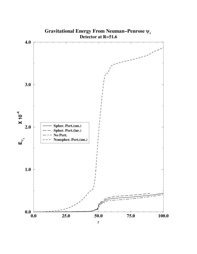
Figure 13: A comparison of gravitational energy output for a star of unperturbed central field density $0.15$ for spherical and nonspherical perturbations. While the level of this ‘background’ is not insignificant it is sufficiently small that the results for the nonspherical perturbations may be trusted.

The energy was also calculated by other means, namely the Bel–Robinson vector $p^{i}$:

$$\frac{dE}{dt}=\frac{1}{4\pi}\int\,\left[\int_{0}^{t}\,dt^{\prime}\left(\pm\sqrt{|p^{x}x+p^{y}y+p^{z}z|/2}\right)\right]^{2}r^{2}d\Omega,$$ (49)

as well as from the Zerilli functions $\Psi_{Z}$:

$$\frac{dE}{dt}=\frac{1}{32\pi}\left(\frac{\partial\Psi_{Z}}{\partial t}\right)^{2}.$$ (50)

We show a perturbed stable star with unperturbed central field density $0.1414$ that had been given a very tiny non-spherical perturbation so that we could obtain its quasinormal modes. Fig. 14 shows three plots of the gravitational energy output as detected by three detectors placed at various points on the grid. The first plot shows a Bel–Robinson calculation, the second a Newman–Penrose calculation and the third a Zerilli calculation. While the former two have consistent results the Zerilli plot shows much more sensitivity to detector positioning. That is, boundary effects as well as how close one is to being in a vacuum, seem to affect the Zerilli calculation more than the others. In the case of the Bel–Robinson and Newman–Penrose calculation the outermost detector is most affected by the boundary errors, while the other two give curves that flatten out. In Fig. 15 we show three plots, each now an energy comparison by the three methods, at a particular detector. The Bel–Robinson and Newman–Penrose calculations are most sensitive to how close one is to being in a vacuum while the Zerilli is most affected by boundary problems. Taking the middle detector as the best compromise between boundary effects and degree of vacuum, we see that the Bel–Robinson and Newman–Penrose calculations match up very well for the most part until the point where they level off, with about $12\%$ differences at levelling off positions.

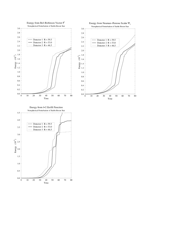
Figure 14: The gravitational wave energy output of a non-spherically perturbed stable boson star of central field density $0.1414$ is shown as measured at three detectors at the outer region of the grid. Three plots are shown, the first showing measurements using the Bell–Robinson vector, the second using the Newman–Penrose $\Psi_{4}$ parameter and the third using the Zerilli functions. The most erratic are the Zerilli measurements.

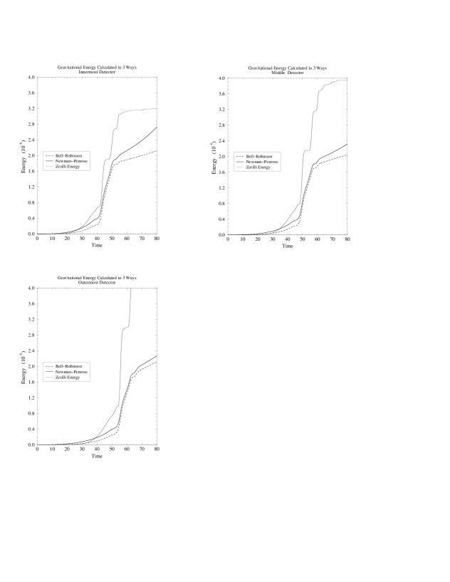
Figure 15: A comparison of the gravitational energy output using the three measures defined in the previous figure is made at three detectors for the non-spherically perturbed stable star described in the previous figure. While the Bel–Robinson and Newman–Penrose $\Psi_{4}$ calculations are quite close the Zerilli data is more erratic.

The scalar radiation still dominates the system’s energy output as seen in Fig. 16 where we have plotted a tenth of the scalar radiation and the total gravitational energy radiation from Bel–Robinson calculations so as to be able to show them on the same plot. The matter radiation clearly moves out slower. The star’s configuration after it gets rid of the gravitational radiation becomes spherically symmetric, and it continues its evolution through spherical oscillations.

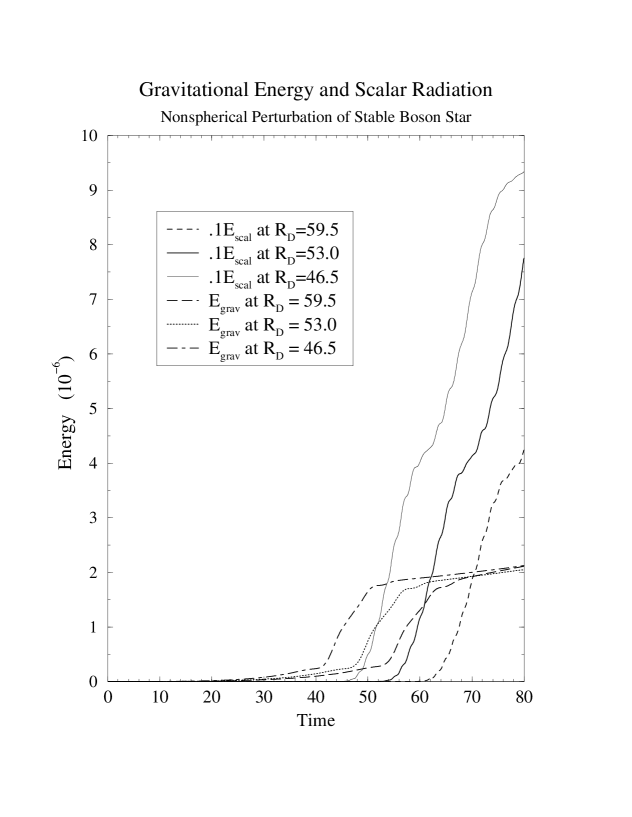
Figure 16: The stable star previously described, when subjected to a nonspherical perturbation, emits gravitational and scalar radiation. The gravitational radiation is far less in amount compared to the dominant scalar energy radiated. The scalar radiation, due to the bosonic matter, travels slower than the gravitational wave due to curvature perturbations.

The nonradial quasinormal modes for the configuration with central field density $0.1414$ have been calculated in [33] using perturbation theory. We have briefly described this in the introduction of this thesis. We have looked at our Newman–Penrose $\Psi_{4}$ function and performed a two-mode fit of their lowest two $l=2$ modes. Our results are shown in fig. 17. Clearly we have a very close agreement to their results. After the first burst of energy, the star moves into the quasinormal mode and stays there till boundary effects become significant.

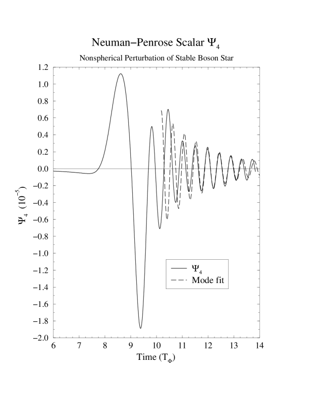
Figure 17: The gravitational waveform $\Psi_{4}$ is shown, as is a quasinormal mode fit for the stable boson star previously described. The star gradually starts oscillating in its quasinormal mode and then at late times boundary effects start affecting the system. The plot has time in units of the underlying oscillation of the scalar field (time period of $2\,\pi$).

We also compared two evolutions of a stable star, one with a small and the other with a large nonspherical perturbation. We observed that the energies of the gravitational waves and scalar radiation were greater in the case of the large perturbation. An infinitesimal perturbation caused the star to oscillate at the quasinormal mode of the original stable star while a substantial perturbation caused it to move to a new configuration, going through the modes of intermediate states. A Fourier transform for a star of central field density $0.15$ with a small and large perturbation exhibits the differences in frequency in Fig. 18.

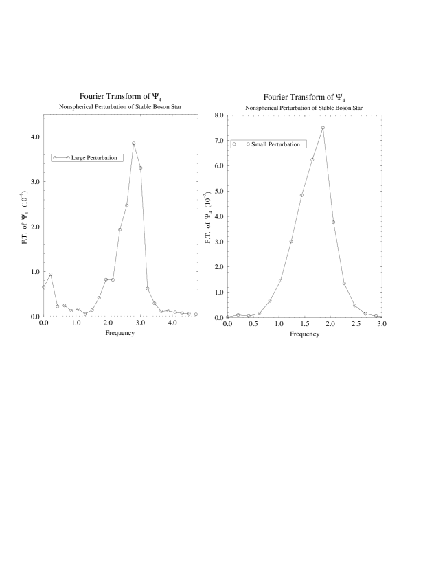
Figure 18: The nonradial modes of a strongly perturbed star are shown to be very different from the nonradial modes of slightly perturbed one. The former star will lose far more mass through scalar and gravitational radiation and move to a new configuration. The latter oscillates in the quasinormal mode of the original configuration.

Thus we have demonstrated that our code gives very consistent results and is capable of providing a detailed description of the gravitational signatures of a boson star.

4.7 Colliding Two Boson Stars

Another project, although still in its infancy, is that of the collision of two boson stars. The $1D$ data of a single star was put on a $3D$ grid using reflection symmetry along an axis to simulate the presence of two identical boson stars. In order to center two stars on the $Z$ axis separated by some number of grid points $2\,nzs$ the boson field $\psi(i,j,nzs-k+1)$ was added to $\psi(i,j,nzs+k)$ to get the new field $\psi(i,j,k)$ for all $i,j,k$ on the grid. As an initial guess metric we just used the one star metric $g_{rr}(i,j,k)=g_{rr}(i,j,nzs-k+1)$ and $g_{00}(i,j,k)=g_{00}(i,j,nzs-k+1)$. We then used the initial solver to get proper initial data assuming the momentum constraints were satisfied (we had time-symmetric data and the $\pi$ fields were defined appropriately). The main result that we have right now, is that because the system produces much more gravitational radiation, the errors in the Zerilli functions due to boundary problems is much less significant. Typically, though, the first two detectors were in close agreement for the Zerilli function and the last two for the Newman–Penrose calculation. This shows the Zerilli function is still somewhat sensitive to outer boundary errors. The disagreement between the the two measures is markedly reduced compared to the earlier cases with smaller signals. So far we have only observed black hole formations from these collisions. These black hole formations were accompanied by negligible amounts of scalar radiation. Steep gradients in the metrics invalidated the code as they could not be resolved as the black hole formed.

In Fig. 19 we show the gravitational energy radiated in the black hole formation during a two boson star collision. The central field density is $0.075$ for the individual stars. One reason to study the two boson star collision is that it is a way to study the generalized two body problem. The amount of energy radiated may not sensitively depend on the component constituents of the collision. An order-of-magnitude calculation of the energy output to mass ratio (of the two boson star configuration) gives a value $\sim 5\times 10^{-4}$ comparing well to the energy emitted ($0.001$) by two black hole collisions for black holes separated by large distances [26].

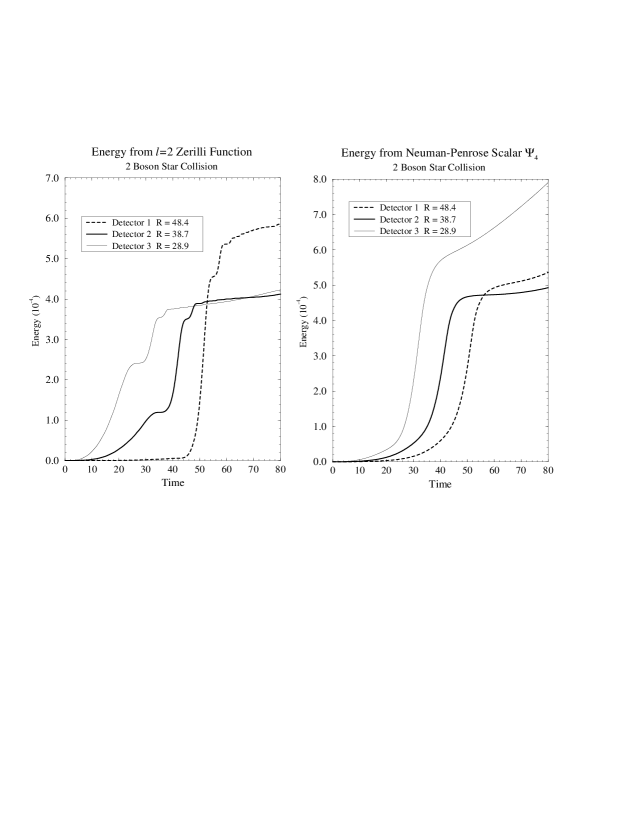
Figure 19: The energy carried by a gravitational wave as measured by three detectors, is shown for a Zerilli calculation and a Newman-Penrose calculation. The former shows very close agreement for the first two detectors but outer boundary effects result in inaccuracies in the third detector’s signal. The latter on the other hand shows a close agreement in the last two detectors’ signals.

4.8 Boson Star: Black Hole Formation

In the spherical collapse problem our $1D$ code with the polar slicing condition caused the lapse to collapse and radial metric to grow uncontrollably at the approach of an apparent horizon. Our code was unable to handle these sharp gradients and crashed (uncontrollable numerical instabilities arose). By using a $3D$ code with maximal slicing, that was still singularity avoiding, but not as drastically as polar slicing, one could confirm the formation of the black hole. We took advantage of the $1D$ code’s ability to resolve the star, by monitoring the first part of its evolution in the $1D$ code. Then after collapse was initiated, and before the gradients got too large, we collected data and placed it on the $3D$ grid. At this stage the star was smaller and the outer part of the grid could be conveniently thrown away allowing us decent resolution in $3D$.

We used “polar slicing” in the $1D$ code, which did not set $TrK=0$ except on the initial time slice. As the system evolved in $1D$ it evolved to $TrK\neq 0$. While maximal slicing ($TrK=0$) avoided problems like grid stretching, by keeping the volume fixed in the absence of a shift, our initial data did not have $TrK=0$. Although the K-driver transformed the slicing to $K=0$ after a short time the evolution exhibited severe grid stretching and we could evolve with zero shift only to a time of $22.6M$ as opposed to $t\sim 50M$ for vacuum Schwarzschild black holes. We present a plot of $g_{rr}$ for the simulation of boson star collapse to a black hole in Fig. 20.

Figure 20: This plot shows the evolution of the radial metric function $g_{rr}$ for the case of the spherical collapse of a boson star to a black hole. In this simulation the shift is zero and the lapse function is obtained by solving the maximal slicing equation with a K-driver term $\sim cK$.

Singularity avoiding slicings offer a way to avoid evolution in regions with singularities while continuing the evolution in regions outside. However they only manage to delay the breakdown of a numerical code. Pathological properties of the slicing, like sharp gradients near the horizon, eventually invalidate the code.

Since the region inside the black hole horizon cannot causally affect the region outside, one can in principle cut away the interior singular region and continue the evolution outside. An outside observer loses no information by cutting away a causally disconnected region. This requires an apparent horizon boundary condition (AHBC).

For a collapsing star this can be implemented by evolving the star under suitable gauge conditions for a while and then introducing a shift vector after an apparent horizon is generated. This shift vector’s function would be to maintain the apparent horizon at some fixed position [67]. This machinery had been developed for black holes [69] and was used in our code to lock the horizon in the spherical collapse problem. The simulation began without AHBC implemented and covered the $r=0$ region. After some evolution the apparent horizon formed and the grid was cut. A B-locking shift as previously described was applied to prevent coordinate drift. The lapse function was updated by a gamma-driver slicing. The details of these conditions and the causal differencing (using one-sided derivatives inside the apparent horizon) can be found in [69] and [67]. With this machinery our code ran twice as long. We show the radial metric evolution in Fig. 4.8.

Chapter 5 Conclusions

Even the skeptic, who refuses to believe in the possibility of the existence of self-gravitating bosons, would be forced to admit that they are indeed very useful objects: That is to say, they are rich in physical content, providing insights into the nature of several physical systems.

For instance the dark matter problem is real and there must be something to explain it. We know that normal baryon densities are not enough to close the universe, and we know that cold and hot dark matter models fail to explain large and small scale structure of the universe, respectively. Relativistic Bosons seem to offer a partial solution to these problems. Although they have particles with high velocities to explain the large scale power spectrum, they have more low velocity particles than fermionic hot dark matter (because of the Bose-Einstein distribution as opposed to the Fermi-Dirac distribution). Thus while small scale power is erased for hot dark matter due to free streaming, enough survives on the smallest scales with this kind of bosonic hot dark matter [18].

Also, many particle physics and cosmological models rely on some form of scalar particles. These unseen scalars could very well be dark matter constituents. From the primordial soup of scalar particles self-gravitating objects can form by the Jeans instability mechanism. Perturbations larger than the Jeans’ length on a homogeneous background could cause the compactification of matter [16].

Self-gravitating objects made from complex scalar fields are called Boson stars. These solutions to the Klein–Gordon–Einstein equations are held together by the balance between attractive forces of gravity and the dispersive forces of the wave equation. In the literature they are referred to as mini-soliton stars [3] because of their small sizes. The addition of a small coupling parameter can however increase their size to neutron star dimensions, making them astrophysically interesting.

The masses of these stars increases with central density up to a peak and then decreases. We have investigated the stability of ground and excited state boson stars with self-coupling [50]. The branch to the left of the peak is called an $S$ or stable branch while the branch to the right is called the $U$-branch. Configurations on the $S$ branch have very specific quasinormal modes of oscillation under small perturbations. Under finite perturbations they settle down to new configurations on the same branch. When perturbed, configurations that lie on the unstable or $U$-branch either migrate to new configurations on the $S$-branch or collapse to black holes. These characteristics are shared by boson stars with or without self-coupling.

Excited states are configurations with nodes. The field of an $n^{\rm{th}}$ excited state star has $n$ nodes and its radial metric has $n+1$ peaks. Their mass profiles are similar to the profiles of boson stars in the ground state, which makes it appear as if they have a stable and an unstable branch of configurations. However, irrespective of which branch they lie on, excited boson stars are unstable with different instability timescales. Low density excited stars having masses close to ground state configurations will form ground state boson stars after evolution. Denser configurations form black holes with the decay time decreasing with increasing central density till one approaches the density corresponding to zero binding energy. As the central density approaches this critical central density the kinetic energy of the star starts to increase as it becomes more dispersive. It still collapses to a black hole but on a larger time scale. Beyond this point, for densities corresponding to positive binding energy, the stars disperse to infinity.

An interesting feature in the collapse of excited state boson stars is that, during this process, they cascade through intermediate states, rather like atoms transiting from excited states to the ground state, suggesting that boson stars behave in some ways like gravitational atoms [54]. However, for boson stars, an investigation of the possible decay channels (selection rules) seems much more difficult (if at all possible or meaningful) due to the intrinsic nonlinearity of the theory.

We have also studied the stability and formation of boson stars in Brans-Dicke theory [56]. The arbitrariness of units of length, time, and masses, and the observed coincidences in the values of dimensionless constants, resulted in alternative theories of gravity, like BD theory and scalar-tensor theories, being propounded. While it has been established that the weak-field differences between these theories and gravity is insignificant at the present times, the question is whether a boson star model can be a source of strong-field differences. We have worked on a BD model, with the view of carrying on the calculation to more general ST theories in the future.

We find the basic features of $U$-branch and $S$-branch stability and excited state transitions to be similar to GR. We do see the BD field, which is static for an equilibrium configuration, begin to oscillate when perturbed, as do the metric components. However these oscillations of the gravitational field are not accompanied by any significant gravitational radiation.

Using a Gaussian initial boson scalar field configuration, to represent the local accumulation of matter, we were able to demonstrate the formation of boson stars in $BD$ theory. This demonstrates that a boson star is a physically realizable object in $BD$ theory.

The flatness of galactic rotation curves indicates the presence of dark halos extending beyond the last visible point, with masses proportional to distance and densities inversely proportional to distance squared. While boson stars in the ground state have too fast a mass fall off to fit galactic rotation curves, third and fourth excited state stars with and without self-coupling have been used to fit them quite well [48], [49]. These states are unstable but their energy differences from lower excited states are large enough to warrant large instability time scales. As we have seen in our own simulations, a repulsive self interaction term further increases this instability time scale.

Another model that can explain galactic rotation curves involves massless scalar fields [46], [47]. The dispersive effects of the scalar field prevents collapse of these halos to black holes. These configurations exist for different values of the scalar field oscillation frequency ($\phi\sim e^{i\omega t}$) and for each value of central density. While the value of the central density is related to the orbital velocity, the scalar field oscillation frequency determines the mass and energy density. The Newtonian configurations had already been described and we studied the stability and formation of these objects in a relativistic code[45]. The mass and energy densities still had the desirable properties for flattening out rotation curves.

We have also shown that massless complex scalar fields are able to settle down to a stable configuration. It seems that the formation process needs a special profile for the energy density. The appearance of points of inflexion within the decreasing density supports the ‘birth’ of the boson halos. In contrast, extremal values for the density cannot be compensated and lead to the destruction of the initial configuration. Stable configurations cannot be formed from initial Gaussian distributions. This could mean that the formation of boson halos could be difficult. However under perturbations a known stable solution settles to a new one.

The thing that makes these models undesirable though is that they are not asymptotically flat. The cut-off radius of these configurations is quite arbitrary. It could be that the size of the halo depends on the value of the cosmological constant. We are working on boundary conditions to make this model more viable. In the process of studying these solutions we have found similar solutions for the massive scalar field. These solutions have energy density characterized by a series of maxima and minima rather than saddle points. They have positive binding energy and as expected disperse in our numerical simulations.

We have furthermore investigated boson stars in a general three-dimensional code demonstrating the key role that boson stars play in the field of numerical relativity. By exploiting the difference between boson stars and neutron stars, we have managed to deal with them numerically. There are no surface problems in a boson star system. Nevertheless the similarities in their structures has allowed us to study stellar dynamics using them as a model.

On the numerical front we have developed a fully relativistic code with matter sources. By comparisons to known results, we have been convinced that the code is indeed stable within the computational resources available to us. We have tested our scalar evolver by itself and seen that it is stable for thousands of timesteps. We have seen metric components remain static for equilibrium boson stars, for several time steps before outer boundary problems invalidate the code. The amount of scalar radiation under spherical perturbations matches very well with our $1D$ code until boundary reflections become significant. We have observed one full metric oscillation of the quasinormal mode under spherical perturbations.

We have then moved a step further to study real physics with this code by studying the behavior of boson stars under non-spherical perturbations. We have measured the gravitational wave output using different techniques with comparable results. We have calculated the quasinormal modes of the star under infinitesimal perturbations. Our results are consistent with those of [33]. The nonradial modes for boson star configurations are strongly damped. This allows us to get the full gravitational wave output for these stars in a relatively short evolution timescale. After the emission of gravitational waves the star becomes spherical and then oscillates in its spherical quasinormal mode. The amount of scalar radiation is much more than the gravitational radiation for these configurations. The scalar radiation decouples from the gravitational radiation. While the latter propagates at the speed of light the scalar radiation is slower and arrives later at our detectors. Under larger non-spherical perturbations the star emits more radiation and does not oscillate in the quasinormal mode of the initial configurations. By comparing the amount of gravitational radiation for unperturbed, spherically perturbed, and non-radially perturbed configurations, we have convinced ourselves that numerically induced asymmetries are negligible.

We have collided two boson stars and formed black holes. This is with the view of studying the generalized two-body problem in $GR$. The amount of scalar radiation in these black hole collapses is negligible and the gravitational radiation dominates the system. The ratio of energy radiated to initial mass of the system is of order $0.0005$ as opposed to $0.001$ for two black hole collisions initially largely seperated. These numbers are comparable and might suggest that the two body problem may be independent of the nature of the constituent objects. Thus a boson system might, with its absence of singularities and surface problems, be ideal to study such systems.

We have also seen the collapse to black holes of unstable boson stars. This is of importance on two accounts. When we performed these simulations in $1D$ we used a polar-slicing condition which caused the lapse to collapse and radial metric to blow up at the approach of an apparent horizon. Thus we could not carry the simulation through to actual black hole formation . By using a maximally-sliced $3D$ code we can carry our simulation further and confirm black hole formation. In addition by running the $1D$ code with very fine resolution until gradients start getting steep and collapse has been initiated, we could throw away the outer part of the star (its radius has been reduced due to collapse). It could then be placed on a $3D$ grid with finer resolution than if we started the simulation from the beginning in $3D$. After this we could turn on the $AHBC$ and evolve the resulting black hole with matter present in the space-time. This added a new dimension to the black hole problem.

Thus with a simple system of bosons, we have touched upon numerous physical and numerical issues. We now have stable $1D$ and $3D$ codes that are capable of handling different system configurations. There are several models whose equilibrium configurations have been described but whose evolutions have not been studied.

For example we have considered boson stars which are minimally coupled to gravity. If one considers the relevance of boson stars in the early universe, it would be worth investigating scalar fields non-minimally coupled to gravity. Since the Pecci-Quinn symmetry [70] is not exact, QCD effects place the coupling strength for axions at $\xi\approx 10^{-20}$ (not 0). This concept might extend to complex scalar fields. In [71] a nonminimal coupling of the form $\xi\,|\phi|^{2}R$ is chosen and the equilibrium configurations are described. For a coupling strength $\xi>4.0$ the mass is always less than the particle number. One expects the branch to the right of the maximum mass to be unstable but if the particle number is greater than the mass this instability must always manifest itself in gravitational collapse and not dispersion. These things can only be confirmed in an evolution code.

There are also descriptions of the equilibrium sequences of mixed fermion-boson stars [72, 73]. Pure boson stars are qualitatively quite similar to pure fermion stars. A mixture of bosons and fermions interacting only by gravitational forces is of interest in field theory as a study of the self-confinement of two quantum fields [72]. Also bosonic axion fields could be captured by neutron stars and influence their stability. Similarly nuclear matter in high density neutron cores could be subject to phase transitions into the pion condensate. Again the stabilities and behavior of the system can be studied only in an evolution code.

One interesting project would be to confirm whether real scalar field configurations could exhibit long term stability under non-spherical perturbations. While these configurations had no static equilibrium solutions [74, 75, 76], periodic solutions have found [77]. Evolution studies in a $1D$ code showed that there were oscillating configurations that oscillated about some configuration for a long time, without observable diminishing mass. This study could be taken to the next step by studying the behavior of the system under more realistic non-spherical perturbations. Since axions are described by real fields this would be of particular importance.

The list is endless and one hopes that the tools described and developed in this thesis will make their contribution in furthering knowledge in physics and numerical relativity.

Appendix: Scaling

In transferring initial $1D$ data from the $1D$ boson star code, to the $3D$ “G” code, where it was interpolated onto a $3D$ grid and evolved, one had to make sure all coordinates were rescaled appropriately. Essentially this meant going from a code where $\hbar=1$ and $c=1$ (the $1D$ code) to a code where $G=1$ and $c=1$. In terms of coordinates this translates to the spatial coordinates going from units of inverse mass to units of mass. Consider for example the $1D$ Hamiltonian constraint.

$$g^{\prime}=\frac{1}{2}\left[\frac{g}{{\bf r}}-\frac{g^{3}}{{\bf r}}+4\pi G\left[m^{2}\phi^{2}{\bf r}g^{3}+\dot{\phi}^{2}{\bf r}g^{3}/N^{2}+{\bf r}g{\phi^{\prime}}^{2}\right]\right].$$ (1)

In dimensionless coordinates ($r$, $t$, $\sigma$, and $N$)

$$r=m{\bf r},\quad t=\omega_{0}{\bf t},\quad\sigma=\sqrt{4\pi G}\phi,\quad N={\bf N}\frac{m}{\omega_{0}},$$ (2)

where $m$ refers to the mass of a boson and $\omega_{0}$ the oscillation frequency of the boson field, this becomes

$$g^{\prime}=\frac{1}{2}\left[\frac{g}{r}-\frac{g^{3}}{r}+rg^{3}\left[\sigma^{2}+\frac{\dot{\sigma^{2}}}{N^{2}}\right]+rg{\sigma^{\prime}}^{2}\right].$$ (3)

Since the field is very small at the edge of the grid the metric components can be taken to be Schwarzschild there. So $g^{2}(\infty)\sim{1}/(1-{2MG}/{\bf r})$. This means the mass of the star is given by

$$M=\frac{{\bf r}}{2G}\left(1-\frac{1}{g^{2}}\right),$$ (4)

calculated at the edge of the grid.

Using $\frac{c\hbar}{G}=M_{Pl}^{2}$ (for the $1D$ code therefore $G=1/M_{Pl}^{2}$) and ${\bf r}=r/m$, where $r$ is the dimensionless radius read off from the output of the $1D$ code, we get

$$M=\frac{r}{2}\left(1-\frac{1}{g^{2}}\right)\,\frac{M_{Pl}^{2}}{m}.$$ (5)

Going back to equation (2), one sees that when the code runs for a certain dimensionless time $t_{\mathrm{c}ode}$ it corresponds to physical time ${\bf t}=1/\omega_{0}\,t_{\mathrm{c}ode}=\frac{N}{{\bf N}m}\,t_{\mathrm{c}ode}$, where $\omega_{0}$ has been written in terms of the lapse. For a boson star of mass $0.633\,M_{Pl}^{2}/m$ (maximum mass of a ground state star) we can compute the physical time

$${\bf t} = \frac{1}{0.633}\frac{N}{{\bf N}}\,G\,M\,t_{\mathrm{c}ode},$$ (6)

$$= \frac{1}{0.633}\,\left(\frac{m\,c^{2}}{{\hbar\,\omega_{0}}}\right)\,\left(\frac{G\,M}{c^{3}}\right)\,t_{\mathrm{c}ode},$$ (7)

where we have written the mass of the boson in terms of the mass of the star (Schwarzschild radius of the star $\sim 1/m$). Computing $\frac{N}{{\bf N}}$ at the edge of the grid, where ${\bf N}\sim\sqrt{1-2M/r}$, we find this fraction to be of order 1. Thus 1 unit of code time in terms of the mass of the star is about $1.6\,GM/c^{3}$.

In the $3D$ code however G=1 but $\hbar$ is not. So consider the Hamiltonian constraint equation again. There is no special reason for this but it suffices to use it to figure out the scaling parameters. Every derivative must be multiplied by $\hbar$, which had been set equal to 1 in the $1D$ case. Now $G$ is set equal to 1. So one has for the Hamiltonian constraint equation

$$g^{\prime}=\frac{1}{2}\left[\frac{g}{{\bf r}}-\frac{g^{3}}{{\bf r}}+4\pi\left[m^{2}\phi^{2}{\bf r}g^{3}+\hbar^{2}\dot{\phi}^{2}{\bf r}\frac{g^{3}}{N^{2}}+{\bf r}g\hbar^{2}{\phi^{\prime}}^{2}\right]\right],$$ (8)

substituting dimensionless coordinates

$$r=m{\bf r}/\hbar,\quad t=\omega_{0}{\bf t},\quad\sigma=\sqrt{4\pi}\hbar\phi,\quad N={\bf N}\frac{m}{\hbar\omega_{0}},$$ (9)

we get back equation (3). Now to interpret our results, which have thus far been stated as raw dimensionless numbers: Without metric evolution the code runs to a time of 2000. The more complete problem must include metric evolutions. For this case, when we have in our reports been stating that the code runs to a time of 140, we actually mean that the code runs to a time of $140/\omega_{0}$ with $1/\omega_{0}=\hbar/m\frac{N(\infty)}{{\bf N}(\infty)}$. In $G=1$ units we have

$$M=\frac{{\bf r}}{2}\,\left(1-\frac{1}{g^{2}}\right),$$ (10)

calculated at the edge of the grid. This gives

$$M=\frac{r}{2}\,\left(1-\frac{1}{g^{2}}\right)\,\frac{\hbar}{m}.$$ (11)

Using the fact that $G=1$ and $c=1$ implies $\hbar=M_{Pl}^{2}$ one gets the same result as before. That is

$$M=\frac{r}{2}\,\left(1-\frac{1}{g^{2}}\right)\,\frac{M_{Pl}^{2}}{m},$$ (12)

which for the problem in consideration is $M=0.05\,M_{Pl}^{2}/m$. Replacing for $1/m$ in the equation for $1/\omega_{0}$ gives $1/\omega_{0}=\frac{N(\infty)}{{\bf N}(\infty)}\frac{M}{0.05}$ where the $\hbar$ cancels the factor $M_{Pl}^{2}$. $N$ is $>1$ and ${\bf N}<1$ with the ratio slightly greater than 1. So an order of magnitude for 1 time step in terms of mass for the maximum mass boson star is $1/0.633\sim 1.6$ times the mass of the star.

For our equilibrium configurations with full evolutions we use star masses of order $0.5\,M_{Pl}^{2}/m$ so one time step is slightly more than two times the mass of a star. The code runs to a dimensionless time of over $500$ or over thousand times the mass of the star ($t_{\mathrm{p}hysical}>1000\,GM/c^{3}$).

For non-spherical perturbations the mass was of order $0.584\,M_{Pl}^{2}/m$. One time step was roughly 1.87 times the mass of the star.

Bibliography

- [1] D.J. Kaup, Phys. Rev. 172, 1331 (1968).
- [2] R. Ruffini and S. Bonnazola, Phys. Rev. 187, 1767 (1969).
- [3] T.D. Lee and Y. Pang, Nucl. Phys. B315, 477 (1988).
- [4] T.D. Lee and Y. Pang, Phys. Rev. D35, 3678 (1987).
- [5] C.W. Misner, K.S. Thorne, and J.A. Wheeler, Gravitation (W.H. Freeman, San Francisco, 1973).
- [6] J. Balakrishna, E. Seidel and W.-M. Suen, “Self gravitating bosons.” Review article to be submitted to Class. Quantum Gravity
- [7] J.A. Wheeler, Phys. Rev. 97, 511 (1955).
- [8] J.L. Basedevant, A. Martin, and J.M. Richard, Nucl. Phys. B343, 60 (1990).
- [9] M. Membrado, A.F. Pancheco, and J. Sanado, Phys. Rev. A39, 427 (1988).
- [10] M. Merafina and R. Ruffini, Astron. and Astrophysics, 221, 4 (1989).
- [11] G. Ingrosso and R. Ruffini, Nuovo Cimento B101, N4 (1988).
- [12] R. Friedberg, T.D. Lee, and Y. Pang, Phys. Rev., D35, 3640 (1987).
- [13] M. Colpi, S.L. Shapiro, and I. Wasserman, Phys. Rev. Lett. 57, 2485 (1986).
- [14] M. Gleiser, Phys. Rev. D38, 2376 (1987).
- [15] R.L. Bowers and E.P.T. Liang, Astrophys. J. 188, 657 (1974).
- [16] J. Binney and S. Tremaine, Galactic Dynamics (Princeton University Press, 1987).
- [17] P.J.E. Peebles, Principles of Physical Cosmology (Princeton University Press, 1993).
- [18] J. Madsen, Astrophysical Journal 371, L47–L49 (1991).
- [19] S. Weinberg, Gravitation and Cosmology (John Wiley and Sons, New York, 1972).
- [20] T. Regge and J.A. Wheeler, Phys. Rev. 108, 1063 (1957).
- [21] A. Abrahams, D. Bernstein, D. Hobill, E. Seidel, and L. Smarr, Phys. Rev. D45, 3544 (1992).
- [22] V. Moncrief, Ann. Phys. (N.Y.), 88, 323 (1974).
- [23] F.J. Zerilli, Phys. Rev. Lett 24, 737 (1970); Phys. Rev. D2, 2141 (1970).
- [24] E. Newman and R. Penrose, J. Math. Phys. 3, 566 (1962).
- [25] L. Smarr, in Sources of Gravitational Radiation. Edited by L. Smarr (Cambridge University Press, Cambridge, England, 1979), p. 245.
- [26] P. Anninos, D. Hobill, E. Seidel, L. Smarr, and W.-M. Suen, Phys. Rev. D52, 2044 (1995).
- [27] V.D. Zakharov, Grav. Waves in Einstein’s Theory (Halsted Press, New York, 1973).
- [28] S. Yoshida, and Y. Erguchi, Phys. Rev D55, 1994 (1996).
- [29] S. Yoshida, and Y. Erguchi, Phys. Rev D56, 762 (1997).
- [30] Y. Kobayashi, N. Kasai, and T. Futamase, Phys. Rev. D50, 7721 (1994).
- [31] F.E. Schunck, and E.W. Mielke, Relativity and Scientific Computing. Edited by F.W. Hehl, R.A. Puntigam, and H. Ruder (Springer, Berlin, 1996), p. 138.
- [32] F.D. Ryan, Phys. Rev. D55, 6081 (1997).
- [33] S. Yoshida, Y. Erguchi, and T. Futamase, Phys. Rev. D50, 6235 (1994).
- [34] K.D. Kokkotas and B.F. Schutz, Gen. Rel. Grav. 18, 913 (1986).
- [35] E. Seidel and W.-M. Suen, Phys. Rev. D42, 384 (1990).
- [36] J. York, in Sources of Gravitational Radiation. Edited by L. Smarr (Cambridge University Press, Cambridge, England, 1979), p. 83.
- [37] L. Smarr, in Sources of Gravitational Radiation. Edited by L. Smarr (Cambridge University Press, Cambridge, England, 1979), p. 139.
- [38] J.M. Bardeen and T. Piran, Phys. Rep. 96, 205 (1983).
- [39] P. Jordan, Nature 4172, 637 (1949).
- [40] C. Brans and R.H. Dicke, Phys. Rev. 124, 925 (1961).
- [41] G. Magnano and L.M. Sokolowski, Phys. Rev. D50, 5039 (1993).
- [42] R.H. Dicke and H.M. Goldenberg, Phys. Rev. Lett. 18, 313 (1967).
- [43] R.D. Reasenberg, I.I. Shapiro, P.E. MacNeil, R.B. Goldstein, J.C. Breidenthal, J.P. Brenkle, D.L. Cain, and T.M. Kaufman, Astrophys. J. 234 (1979), L219.
- [44] R.N. Treuhaft and S.T. Lowe, Astrophys. J. 102, 1879 (1991).
- [45] J. Balakrishna and F.E. Schunck, gr-qc 9802054. “Gravitational evolution and stability of boson halos”
- [46] F.E. Schunck, Selbstgravitierende Bosonische, Ph.D. thesis, Univ. of Cologne (Cuvillier Verlag, Göttingen 1996).
- [47] F.E. Schunck, “Massless scalar field models rotation curves of galaxies”, in Aspects of dark matter in astro- and particle physics. Edited by H.V. Klapdor-Kleingrothaus and Y. Ramachers (World Scientific Press, Singapore, 1997).
- [48] S.J. Sin, Phys. Rev. D50, 3650 (1995).
- [49] Jae-weon Lee and In-gyu Koh, Phys. Rev. D53, 2236 (1996).
- [50] J. Balakrishna, E. Seidel, and W.-M. Suen, Phys. Rev. D58, 104004 (1998).
- [51] W.H. Press, S.A. Teukolsky, W.T. Vetterling, and B.P. Flannery in Numerical Recipes in Fortran, edited by L. Smarr (Cambridge University Press, Cambridge, England, 1986).
- [52] G.L. Comer and H. Shinkai, Class. Quantum Grav. 15, 669 (1998).
- [53] P. Jetzer, Phys. Rep. 220, 183 (1992).
- [54] A.R. Liddle and M.S. Madsen, Int. J. Mod. Phys. D1, 101 (1992).
- [55] F.V. Kusmartsev, E.W. Mielke, and F.E. Schunck, Phys. Rev. D43, 3895 (1991).
- [56] J. Balakrishna and H. Shinkai, Phys. Rev. D58, 044016 (1998).
- [57] J. Novak, Phys. Rev. D57, 4789 (1998).
- [58] J. Balakrishna, G. Daues, E. Seidel, and W-M. Suen, in preparation.
- [59] M. A. Scheel, S. L. Shapiro and S. A. Teukolsky, Phys. Rev. D51 4208 (1995); ibid. D51 4236 (1995).
- [60] E. Seidel and W.-M. Suen, Phys. Rev. Lett. 72, 2516 (1994).
- [61] E. Seidel and W.-M. Suen, Phys. Rev. Lett. 72, 2516 (1994).
- [62] D. Christodoulou, Comm. Math. Phys. 105, 337 (1986); Comm. Math. Phys. 109, 613 (1987).
- [63] Ph. Jetzer, Nucl. Phys. B316, 411 (1989); Phys. Lett. B231, 433 (1989).
- [64] M. Gleiser and R. Watkins, Nucl. Phys. B319, 733 (1989).
- [65] T. Piran, in Gravitational Radiation. Edited by N. Deruelle and T. Piran (North-Holland, Amsterdam, 1982), p. 203.
- [66] P. Anninos, K. Camarda, J. Massó, E. Seidel, W.-M. Suen, and J. Towns, Phys. Rev. D52, 2059 (1995).
- [67] P. Anninos, G. Daues, J. Massó, E. Seidel, and W.-M. Suen, Phys. Rev. D51, 2059 (1994).
- [68] J. Balakrishna, G. Daues, M. Tobias, W.-M. Suen, and E. Wang, Class. Quantum Grav. 13 (1996) L135-L142.
- [69] G. Daues Ph.D. thesis Washington University, unpublished.
- [70] R.D. Peccei and H. Quinn, Phys. Rev. Lett. 38, 1440 (1977).
- [71] J.J. van der Bij and M. Gleiser, Phys. Lett.
- [72] G. Ingrosso, D. Grasso, and R. Ruffini, Astron. and Astrophysics 248, 481 (1991).
- [73] A.B. Henriques, A.R. Liddle, and R.G. Moorhouse, Nucl. Phys. B337, 737 (1990).
- [74] G. Rosen, Journal Math. Phys. 7, 2066 (1966).
- [75] G. Rosen, Journal Math. Phys. 9, 996 (1968).
- [76] P. Jetzer and D. Scialom, gr-qc/9709056. “On the stability of real scalar boson stars”
- [77] E. Seidel and W.-M. Suen, Phys. Rev. Lett. 66, 1659 (1990).