Dual-resonator speed meter for a free test mass

Abstract

A description and analysis are given of a “speed meter” for monitoring a classical force that acts on a test mass. This speed meter is based on two microwave resonators (“dual resonators”), one of which couples evanescently to the position of the test mass. The sloshing of the resulting signal between the resonators, and a wise choice of where to place the resonators’ output waveguide, produce a signal in the waveguide that (for sufficiently low frequencies) is proportional to the test-mass velocity (speed) rather than its position. This permits the speed meter to achieve force-measurement sensitivities better than the standard quantum limit (SQL), both when operating in a narrow-band mode and a wide-band mode. A scrutiny of experimental issues shows that it is feasible, with current technology, to construct a demonstration speed meter that beats the wide-band SQL by a factor 2. A concept is sketched for an adaptation of this speed meter to optical frequencies; this adaptation forms the basis for a possible LIGO-III interferometer that could beat the gravitational-wave standard quantum limit $h_{\rm SQL}$, but perhaps only by a factor $1/\xi=h_{\rm SQL}/h\lesssim 3$ (constrained by losses in the optics) and at the price of a very high circulating optical power — larger by $\xi^{-2}$ than that required to reach the SQL.

I Introduction

A conceptual design for a quantum speed meter was proposed several years ago [1]. This speed meter couples to the velocity of a free test mass and thereby can monitor a classical force that acts on the test mass with a precision better than the Standard Quantum Limit (SQL).

The motivation for coupling to test-mass velocity rather than position is that (in the absence of the coupling) the test-mass velocity is equal to momentum divided by mass; and momentum, by contrast with position, is a constant of the test mass’s free motion, so it commutes with itself at different times and is a quantum nondemolition (QND) observable [2]. This enables the speed meter to beat the classical-force SQL without any special squeezed-state preparation of the speed meter’s microwave pump field or frequency-dependent homodyne detection of its output signal field. By contrast, to beat the classical-force SQL, a meter that couples to position must incorporate a squeezed-state pump and/or frequency-dependent homodyne detection; see Appendix A.

In Ref. [1] two variants of the speed meter were suggested, one based on an optical-fiber delay line and the other on coupled microwave resonators (“dual resonators”). In this paper we analyze in detail the dual-resonator scheme and show that it can be realized in principle with current experimental technology.

An important possible application of this speed meter is as the readout device for a new class of laser-interferometer gravitational-wave antennas that may beat the SQL while using unusually low laser power [3, 4, 5].

The speed meter proposed in Ref. [1] is based on two identical, weakly coupled microwave resonators as shown in Fig. 1. It is a fascinating characteristic of such coupled resonators that, when one is driven at their common eigenfrequency $\omega_{e}$, it is the other that becomes excited. Resonator 2 is pumped on resonance by the voltage $U_{0}\cos\omega_{e}t$ of an input waveguide, so resonator 1 becomes excited at frequency $\omega_{e}$. The eigenfrequency of resonator 1 is modulated by the position $x$ of the test mass

$$\tilde{\omega}_{e}(x)=\omega_{e}\left(1-\frac{x}{d}\right),$$ (1)

where $d$ is a length that characterizes the resonator’s tunability (cf. Sec. V); this modulation puts a voltage signal proportional to position $x$ into resonator 2, and a voltage signal proportional to velocity $dx/dt$ into resonator 1. The velocity signal flows from resonator 1 into an output waveguide, from which it is monitored.

FIG. 1.: Schematic diagram of the coupled-resonator quantum speed meter.

One can understand the production of this velocity signal as follows: The weak coupling between the resonators causes voltage signals to periodically slosh from one resonator to the other at the frequency $\Omega\ll\omega_{e}$. After each cycle of sloshing, the sign of the signal is reversed, so the net signal in resonator 1 is proportional to the difference of the position at times $t$ and $t+2\pi/\Omega$, i.e. is proportional to the test-mass velocity so long as the the test mass’s frequencies $\omega$ of oscillations are $\omega\ll\Omega$.

Actually, we shall find that the optimal regime of operation for the speed meter is at signal frequencies $\omega\sim\Omega$. In this regime, the voltage signal in resonator 1 and the corresponding output voltage signal are sums over time derivatives of the test-mass position [Eqs. (37–41)]. Correspondingly, the speed meter does not monitor just the speed, but rather the speed plus time derivatives of the speed.

In this paper we shall analyze in detail the operation of the speed meter, first ignoring the resonators’ dissipative losses and associated noise (Sec. III), then including the losses and noise (Sec. IV). We shall express the speed meter’s performance in terms of the spectral density $S(\omega)$ of the net noise that it produces when monitoring a classical signal force $F_{s}(t)$ that is acting on the test mass. As a foundation for this, in Sec. II we discuss the SQL for force measurements in the language of spectral density. In Sec. V we discuss the most serious practical impediments to achieving a sensitivity that actually beats the SQL by a significant factor and conclude that a demonstration experiment is feasible with current technology. In Appendix A we compare this speed meter with a position meter based on a single microwave resonator with homodyne readout in the output waveguide at a frequency-dependent homodyne phase (“quantum variational technique”); and in Appendix B we describe a speed-meter-based conceptual design for a LIGO-type gravitational-wave antenna that can beat the gravitational-wave SQL, but requires very high light power.

II Standard Quantum Limits

The standard quantum limits (SQL) for measurement of a classical signal force $F_{s}(t)$ acting on a free test mass, as usually given in the literature (e.g. [2]), are not convenient since they are based on some assumed shape of the force’s time dependence (most commonly a single-cycle sinusoid or a long, monochromatic wave train). In this paper we prefer the greater generality of a SQL expressed in terms of the two sided spectral density $S(\omega)$ for the net noise in a measurement of $F_{s}(t)$; $S(\omega)$ is defined such that for optimal signal processing the measurement’s power signal to noise ratio is

$${S\over N}=\int_{-\infty}^{\infty}{|F_{s}(\omega)|^{2}\over S(\omega)}{d\omega\over 2\pi}\;.$$ (2)

Here $F_{s}(\omega)$ is the Fourier transform of $F_{s}(t)$

$$F_{s}(t)=\int_{-\infty}^{\infty}F_{s}(\omega)e^{-i\omega t}{d\omega\over 2\pi}\;,$$ (3)

in which we adopt the $2\pi$ convention of signal processing theory and microwave technology, and the $e^{-i\omega t}$ sign convention of quantum physics (so field amplitudes and annihilation operators evolve as $e^{-i\omega t}$ in the Heisenberg Picture).

A Wideband SQL

An ordinary position meter (sometimes called coordinate meter) monitors the position $x(t)$ of a free test mass, and thereby deduces the classical signal force $F_{s}(t)$ that acts on the mass. The spectral density of the net noise in this force monitoring is

$$S(\omega)=m^{2}\omega^{4}S_{x}+S_{F}\;,$$ (4)

where $m$ is the mass of the test mass, $S_{x}(\omega)$ is the spectral density of the noise $x_{\rm m}(t)$ that the meter superimposes on the output position signal, and $S_{F}(\omega)$ is the spectral density of the fluctuating back-action force $F_{\rm BA}(t)$ that the meter exerts on the test mass. For an ordinary position meter, $x_{\rm m}(t)$ and $F_{\rm BA}(t)$ are uncorrelated, and the Heisenberg uncertainty principle implies that $S_{x}S_{F}\geq\hbar^{2}/4$ [2]. We shall assume that the position meter is as perfect as possible, corresponding to equality in this uncertainty relation. If the spectrum of the classical force is concentrated near the frequency $\omega_{F}$ and the position meter is optimally tuned for monitoring this force (so the ratio $S_{F}/S_{x}$ is adjusted to make the two terms in Eq. (4) equal at $\omega=\omega_{F}$), then the net spectral density is

$$S(\omega) = \hbar m\omega^{2}\quad\mbox{ for }\omega=\omega_{F}\;,$$ (5)

$$S(\omega) \geq \hbar m\omega^{2}\quad\mbox{ for other values of }\omega\;.$$ (6)

This is the spectral-density form of the SQL. The corresponding minimum detectable amplitude for a force that lasts for a time $\tau_{F}$ is

$$F_{\rm WB\ SQL}\simeq\sqrt{\frac{\hbar m\omega_{F}^{2}}{\tau_{F}}}\;.$$ (7)

This is the usual form of the wide-band SQL for a sinusoidal force.

In order for the meter to beat this usual wide-band SQL by a factor $\xi_{\rm WB}<1$,

$$F\simeq\xi_{\rm WB}F_{\rm WB\ SQL},$$ (8)

the spectral density of the net noise must obey the condition

$$S(\omega)=\xi_{\rm WB}^{2}\hbar m\omega^{2}$$ (9)

in the range of frequencies of the detected force. We shall regard Eq. (9) as a definition of the amount $\xi_{\rm WB}(\omega)$ by which our speed meter beats the broad-band SQL.

B Narrowband SQL

If the test mass has a restoring force so it is an oscillator with eigenfrequency $\omega_{0}$, and/or the noises $x_{\rm m}(t)$ and $F_{\rm BA}(t)$ are correlated (with cross spectral density $S_{xF}$), then the net noise in the measurement of $F_{s}(t)$ is

$$S(\omega)=m^{2}(\omega^{2}-\omega_{0}^{2})^{2}S_{x}-2m(\omega^{2}-\omega_{0}^{2})S_{xF}+S_{F}\;.$$ (10)

For such a system, the noise can be made especially small in a narrow-band measurement centered on the frequency

$$\omega_{\rm meter}^{2}=\omega_{0}^{2}+\frac{S_{xF}}{mS_{x}}\;.$$ (11)

If the noises $S_{x}$ and $S_{F}$ can be regarded as constant over that narrow band, and they are constrained only by the Heisenberg uncertainty relation $S_{x}S_{F}-S_{xF}^{2}=\hbar^{2}/4$ [2]), then

$$S(\omega)=m^{2}(\omega_{\rm meter}^{2}-\omega^{2})^{2}S_{x}+\frac{\hbar^{2}}{4S_{x}}\;.$$ (12)

Suppose, now, that we use such a SQL-limited meter to measure a sinusoidal force with frequency $\omega_{F}\simeq\omega_{\rm meter}$ and with duration $\tau_{F}\gg 2\pi/\omega_{F}$ so the bandwidth of the force is $\Delta\omega=2\pi/\tau_{F}\ll\omega_{F}$. Then, if $S_{x}$ is optimized, the amplitude of the minimum detectable force [as computed by setting $S/N\simeq 1$ in Eq. (2)] is at the narrow-band SQL:

$$F\simeq F_{\rm NB\ SQL}=\frac{1}{\tau_{F}}\sqrt{\hbar\omega_{F}m}\;.$$ (13)

Correspondingly, in order to beat the narrow-band SQL, the meter’s net spectral density (10) in the vicinity of some frequency $\omega_{\rm meter}$ must have the form:

$$S(\omega)=A(\omega_{\rm meter}^{2}-\omega^{2})^{2}+B\;,$$ (14)

where the parameters $A$ and $B$ (whose ratio is adjustable) satisfy

$$AB=\xi_{\rm NB}^{4}\frac{\hbar^{2}m^{2}}{4}\;.$$ (15)

The factor $\xi_{\rm NB}<1$ is the amount by which the minimum detectable force is below the narrow-band SQL (13).

Another viewpoint on $\xi_{\rm NB}$ is the following: Define

$$\bar{S}_{F}\equiv S_{F}-\frac{S_{xF}^{2}}{S_{x}}\;,\quad\bar{L}_{\omega}\equiv L_{\omega}+\frac{S_{xF}}{S_{x}}\;,$$ (16)

where $L_{\omega}$ is the spectral response of the test mass ($L_{\omega}=-m\omega^{2}$ for a free mass and $L_{\omega}=m(\omega_{0}^{2}-\omega^{2})$ for a lossless oscillator). Then the net noise [Eq. (10) with $m(\omega^{2}-\omega_{0}^{2})$ replaced by $-L_{\omega}$] takes the form

$$S(\omega)=\bar{L}_{\omega}^{2}S_{x}+\bar{S}_{F}\;.$$ (17)

If the noises are constrained only by the Heisenberg uncertainty relation, $S_{x}S_{F}-S_{xF}^{2}=S_{x}\bar{S}_{F}=\hbar^{2}/4$, and one chooses $\omega_{\rm meter}$ to be at a zero of $\bar{L}_{\omega}^{2}$, then comparison with Eqs. (14) and (15) reveals the following expression for the amount by which the narrow-band SQL can be beaten:

$$\xi^{2}_{NB}=\left|\frac{\bar{L}_{\omega}}{m(\omega^{2}_{meter}-\omega^{2})}\right|\;.$$ (18)

III Microwave Speed Meter in the Lossless Limit

A Equations of motion and their solution

When we neglect all losses in the test mass and in the resonators (and all associated fluctuating forces), except those due to coupling to the output waveguide, then the equations of motion for the speedmeter of Fig. 1 take the following form [6]:

$$\frac{d^{2}q_{1}(t)}{dt^{2}}+2\delta_{e}\frac{dq_{1}(t)}{dt}+\omega_{e}^{2}\left(1-\frac{x(t)}{d}\right)^{2}q_{1}(t)$$ (20)

$$\quad=2\omega_{e}\Omega q_{2}(t)+2\frac{\omega_{e}}{\rho}U_{e}(t)\;,$$ (21)

$$\frac{d^{2}q_{2}(t)}{dt^{2}}+\omega_{e}^{2}q_{2}(t)=2\omega_{e}\Omega q_{1}(t)+2\frac{\omega_{e}}{\rho}U_{0}\cos\omega_{e}t\;,$$ (22)

$$m{d^{2}x\over dt^{2}}={\rho\omega_{e}\over d}q_{1}^{2}-{\rho\omega_{e}\over 2d}q_{0}^{2}+F_{s}(t)\;.$$ (23)

Here the notation is as follows:

• $\omega_{e}$ is the common (angular) eigenfrequency of the two resonators and $\Omega\ll\omega_{e}$ is the weak-coupling frequency at which energy sloshes between the two resonators;

• $q_{1,2}(t)$ are generalized coordinates of resonators 1 and 2, so defined that the energy in resonator $j$ is

  $$E_{j}={\rho\over 2\omega_{e}}\dot{q}_{j}^{2}+{\rho\omega_{e}\over 2}q_{j}^{2}\;,$$ (24)

  with an overdot representing a time derivative;

• $\rho$ is the characteristic impedance of the resonators;

• $\delta_{e}\equiv 1/2\tau_{e}^{*}$ where $\tau_{e}^{*}$ is the relaxation time of resonator 1 due to energy flowing into the output waveguide;

• $U_{e}$ is the fluctuating voltage imposed on resonator 1 from the output waveguide;

• $U_{0}$ is the driving voltage from the input waveguide, and is assumed to be the result of a very strong waveguide field and a very weak coupling to the resonator, so the waveguide’s fluctuational voltages can be ignored and $U_{0}$ can be regarded as a classical c-number;

• $x(t)$ is the position of the free test mass, $d$ is the tuning length of resonator 1, and $x/d$ is assumed to be so small that $(x/d)^{2}$ can be neglected;

• $F_{s}(t)$ is the classical signal force acting on the test mass;

• $q_{0}$ is the amplitude of the classical excitation of $q_{1}$

  $$q_{0}=-{U_{0}\over\Omega\rho}\;,$$ (25)

  and the constant classical force $-(\rho\omega_{e}/2d)q_{0}^{2}$ [second term in Eq. (23)] is applied to the test mass to counteract the mean radiation pressure force [time average of first term in Eq. (23)].

One can take two points of view on the quantities $q_{1}$, $q_{2}$, $x$, and $U_{e}$: one can regard them as classical quantities, with $U_{e}(t)$ described by a classical spectral density $S_{U_{e}}(\omega)$, in which case Eqs. (III A) are classical equations of motion; or one can regard them as quantum mechanical operators in the Heisenberg picture, in which case Eqs. (III A) are the Heisenberg evolution equations. The two viewpoints will produce the same final conclusions, if one chooses the correct quantum-mechanically-based value for $S_{U_{e}}$. We shall return to this in Sec. III B below.

We resolve $q_{1}$ and $q_{2}$ into their quadrature components

$$q_{1} = (q_{0}+a_{1})\cos\omega_{e}t+b_{1}\sin\omega_{e}t\;,$$ (26)

$$q_{2} = a_{2}\cos\omega_{e}t+\left(-{\delta_{e}\over\Omega}q_{0}+b_{2}\right)\sin\omega_{e}t\;.$$ (27)

Note that the classical input driving voltage $2U_{0}\cos\omega_{e}t$, acting on resonator 2, produces its primary classical excitation $q_{0}\cos\omega_{e}t$ in resonator 1 as was advertised in Sec. I; but there is also a secondary classical excitation in resonator 2 proportional to the loss rate $\delta_{e}$ that was ignored in Sec. I.

The quadrature amplitudes $a_{1,2}$ and $b_{1,2}$ carry the perturbations caused by coupling to the test-mass position and to the output waveguide. We solve for these perturbations by inserting expressions (27) into the equations of motion (III A) and linearizing:

$$\frac{da_{1}(t)}{dt}+\delta_{e}a_{1}(t) = -\Omega b_{2}(t)-\frac{U_{es}(t)}{\rho}\;,$$ (29)

$$\frac{db_{1}(t)}{dt}+\delta_{e}b_{1}(t) = \frac{\omega_{e}q_{0}}{d}x(t)+\Omega a_{2}(t)+\frac{U_{ec}(t)}{\rho}\;,$$ (30)

$$\frac{da_{2}(t)}{dt} = -\Omega b_{1}(t)\;,$$ (31)

$$\frac{db_{2}(t)}{dt} = \Omega a_{1}(t)\;,$$ (32)

$$m{d^{2}x\over dt^{2}} = F_{\rm BA}(t)+F_{s}(t)\;.$$ (33)

Here $U_{ec}$ and $U_{es}$ are the quadrature amplitudes of the fluctuating voltage imposed on resonator 1 from the output waveguide,

$$U_{e}=U_{ec}\cos\omega_{e}t+U_{es}\sin\omega_{e}t\;,$$ (34)

and $F_{\rm BA}(t)$ is the back-action force that the speed meter exerts on the test mass averaged over a microwave period $2\pi/\omega_{e}$,

$$F_{\rm BA}(t)={q_{0}\rho\omega_{e}\over d}a_{1}(t).$$ (35)

In the Heisenberg-picture interpretation of Eqs. (III A), all the functions of time $t$ are quantum operators except the classical force $F_{s}(t)$.

We solve Eqs.  (III A) in the frequency domain using the Fourier-transform conventions of Eq. (3). The frequencies of interest are in the range $|\omega|\ll\omega_{e}$ and can be thought of as side-band frequencies of the microwave carrier $\omega_{e}$. Equations (III A) imply, for the quadrature amplitudes of resonator 1:

$$a_{1}(\omega) = \frac{i\omega U_{es}(\omega)}{\rho{\cal L}(\omega)}\;,$$ (36)

$$b_{1}(\omega) = -\frac{i\omega}{{\cal L}(\omega)}\left(\frac{\omega_{e}q_{0}}{d}x(\omega)+\frac{U_{ec}(\omega)}{\rho}\right),$$ (37)

where

$${\cal L}(\omega)\equiv\Omega^{2}-\omega^{2}-i\omega\delta_{e}\;.$$ (38)

The output-wave voltage entering the output waveguide can be expressed in the form [6]:

$$U^{out}(t) = U_{e}(t)-\frac{2\delta_{e}}{\omega_{e}}\rho\frac{dq_{1}(t)}{dt}$$ (39)

$$= \left[U_{ec}(t)-2\delta_{e}\rho b_{1}(t)\right]\cos\omega_{e}t$$ (41)

$$+\left[U_{es}(t)+2\delta_{e}\rho a_{1}(t)\right]\sin\omega_{e}t\;,$$

where we have ignored the carrier signal $2\delta_{e}\rho q_{0}\sin\omega_{e}t$. When measuring the classical signal force $F_{s}(t)$, the noise will be minimized by monitoring the sidebands of an optimally chosen quadrature component of the output wave. This monitoring can be done via homodyne detection [which, at microwave frequencies, can be achieved by mixing the output wave $U^{\rm out}(t)$ with a strong local-oscillator field $U_{LO}\propto\sin(\omega_{e}t+\Phi)$, where $\Phi$ is the desired quadrature’s phase, then rectifying it and averaging it over a carrier period, and then monitoring its slowly oscillating voltage]. The monitored voltage is then proportional to

$$\tilde{U}(t) = \left[U_{ec}(t)-2\delta_{e}\rho b_{1}(t)\right]\sin\Phi$$ (43)

$$+\left[U_{es}(t)+2\delta_{e}\rho a_{1}(t)\right]\cos\Phi\;.$$

By switching to the frequency domain and using expression (37) for $b_{1}(\omega)$, we obtain the following expression for this monitored voltage in terms of the test-mass position $x(\omega)$ and the noise $x_{\rm m}(\omega)$ added to the position signal by the speed meter:

$$\tilde{U}(\omega)=\frac{2i\omega\omega_{e}\delta_{e}\rho q_{0}\sin{\Phi}}{{\cal L}(\omega)d}\left(x(\omega)+x_{\rm m}(\omega)\right),$$ (44)

where

$$x_{\rm m}(\omega)=\frac{d}{2i\omega\omega_{e}\delta_{e}q_{0}\rho}(\Omega^{2}-\omega^{2}+i\omega\delta_{e})$$ (45)

$$\times\left[U_{ec}(\omega)+U_{es}(\omega)\cot\Phi\right]\;.$$ (46)

Notice that in the limit of weak coupling to the output waveguide $\delta_{e}\ll\Omega$, and for signal frequencies low compared to the resonator sloshing frequency $\omega\ll\Omega$, the monitored voltage is $\tilde{U}(t)\propto[dx/dt+dx_{\rm m}/dt]$; i.e., it is proportional to the test-mass velocity, as expected for a speed meter. However, as we shall see below, the regime of optimal sensitivity is one in which the classical force’s signal frequency is at $\omega\sim\Omega$, so the monitored voltage (44) has a more complicated dependence on test-mass position than simply $dx/dt$.

Equation (33) implies for the test-mass position in the frequency domain

$$x(\omega)=x_{o}\delta(\omega)-{p_{o}\over i\omega m}\delta(\omega)-{F_{\rm BA}(\omega)\over m\omega^{2}}-{F_{s}(\omega)\over m\omega^{2}}\;.$$ (47)

Here $x_{o}$ and $p_{o}$ are integration constants (the test-mass position and momentum in the absence of coupling to the signal force $F_{s}(\omega)$ and to the speed meter), $\delta(\omega)$ is the Dirac delta function, and

$$F_{\rm BA}(\omega)=\frac{i\omega\omega_{e}q_{0}U_{es}(\omega)}{{\cal L}(\omega)d}$$ (48)

is the speed meter’s back-action force; cf. Eqs. (35) and (37).

B Meter and Back-Action Spectral Densities

When thinking about this speed meter in the quantum mechanical Heisenberg Picture, one might be concerned that the nonzero value of the test mass’s two-time commutator $[x(t),x(t^{\prime})]=i\hbar(t^{\prime}-t)/m$ will cause the two-time commutator of the output waveguide’s signal to be nonzero; cf. Eq. (44). If this were so, then we would have to worry about the effects of successive quantum state reductions as each successive bit of signal is collected (via homodyne detection). Fortunately, the monitored quantity is the Hermitian part $\tilde{U}^{h}(t)={1\over 2}\left(\tilde{U}(t)+\tilde{U}^{{\dagger}}(t)\right)$ of a quadrature amplitude $\tilde{U}(t)$ of the output waveguide’s microwave field $U^{\rm out}(t)$. The commutation relations for the electromagnetic field guarantee that this quantity commutes with itself at different times $[\tilde{U}^{h}(t),\tilde{U}^{h}(t^{\prime})]=0$, independently of how the field has interacted with the speed meter. (This is a manifestation of the quantum Markov approximation.) In the case of the speed meter, this vanishing commutator is achieved via an automatic cancellation between the influences of the test-mass position $x(t)$ [which in turn is influenced by the meter’s back-action noise $F_{\rm BA}(t)$] and the meter’s noise $x_{\rm m}(t)$; cf. Eqs. (44)–(48).

Because $[\tilde{U}^{h}(t),\tilde{U}^{h}(t^{\prime})]=0$, we can compute the noise in any measurement with the speed meter by taking expectation values in the initial states of the test mass, resonators, and incoming output-waveguide field $U_{e}$. Moreover, when — as in this paper — we are not interested in making absolute measurements of test-mass position and momentum, but instead are interested only in learning about components of the classical force $F_{s}(t)$ bounded away from zero frequency, our final inferred force and its noise will be independent of the initial test-mass position and momentum $x_{o}$ and $p_{o}$ [cf. Eq. (47) where $x_{o}$ and $p_{o}$ appear only at zero frequency]. In addition, in this section’s model, which ignores the resonators’ intrinsic losses, the resonator dissipation via leakage of field into the output waveguide guarantees that the state of the resonators is determined completely by the initial state of the output waveguide field $U_{e}$.

These considerations imply that the measurement noise will be determined solely by the quantum state of the field $U_{e}$ that impinges on the speed meter from the output waveguide. Throughout this paper, except in Sec. V, we shall assume that this field is in its vacuum state. Correspondingly, the spectral densities and cross spectral density of its quadrature components are

$$S_{U_{c}}(\omega)=S_{U_{s}}(\omega)=\hbar\rho\delta_{e}\;,\quad S_{U_{c}U_{s}}=0\;.$$ (49)

(To deduce these spectral densities from the standard theory of a quantized transmission line or waveguide, one must know that, in the notation of our model, the waveguide impedance is $2\rho\delta_{e}/\omega_{e}$.)

By combining Eqs. (49), (35) and (46) we deduce for the spectral densities of the meter’s position noise and back-action force and their cross spectral density

$$S_{x}(\omega) = \frac{\hbar|{\cal L}(\omega)|^{2}}{2m\omega^{2}\Lambda^{4}\sin^{2}\Phi}\;,$$ (51)

$$S_{F}(\omega) = \frac{\hbar m\Lambda^{4}\omega^{2}}{2|{\cal L}(\omega)|^{2}}\;,$$ (52)

$$S_{xF}(\omega) = -\frac{\hbar}{2}\cot\Phi\;.$$ (53)

Here $\Lambda$ is a frequency that characterizes the strength of the pumping,

$$\Lambda^{4}\equiv\frac{2\omega_{e}W}{md^{2}}$$ (54)

with

$$W=\rho\omega_{e}q_{0}^{2}\delta_{e}$$ (55)

the power supplied to the resonator by the input waveguide and the corresponding power removed through the output waveguide; cf. Eq. (24). Below it will be useful to write $|{\cal L}(\omega)|^{2}$ [Eq. (38)] in the form

$$|{\cal L}(\omega)|^{2}=(\omega^{2}-\omega_{0}^{2})^{2}+\delta_{e}^{2}(\omega_{0}^{2}+\delta_{e}^{2}/4)\;,$$ (56)

where

$$\omega_{0}\equiv\sqrt{\Omega^{2}-\delta_{e}^{2}/2}\;;$$ (57)

$\omega_{0}$ will turn out to be the speed meter’s optimal frequency of operation.

C Wide-band sensitivity with lossless resonators

When one infers the classical signal force $F_{s}(t)$ from the speedmeter’s output $\tilde{U}(t)$, the spectral density of the noise of the inferred $F_{s}$ is

$$S(\omega) = m^{2}\omega^{4}S_{x}(\omega)-2m\omega^{2}S_{xF}(\omega)+S_{F}(\omega)$$ (58)

$$= \hbar m\omega^{2}\xi_{\rm WB}^{2}(\omega);$$ (59)

cf. Eq. (9). Equations (III B) and (59) imply for the amount by which the speed meter beats the wide-band standard quantum limit

$$\xi_{\rm WB}^{2}(\omega)=\frac{|{\cal L}(\omega)|^{2}}{2\Lambda^{4}\sin^{2}\Phi}+\cot\Phi+\frac{\Lambda^{4}}{2|{\cal L}(\omega)|^{2}}.$$ (60)

We shall optimize the homodyne phase $\Phi$ so as to minimize $\xi_{\rm WB}$ at the frequency $\omega_{F}$ around which the signal force $F_{s}(t)$ is concentrated. The optimizing phase is

$$\cot\Phi=-\frac{\Lambda^{4}}{|{\cal L}(\omega_{F})|^{2}}\;,$$ (61)

$\xi^{2}_{\rm WB}(\omega)$ for this $\Phi$ is

$$\xi_{\rm WB}^{2}(\omega)=\frac{|{\cal L}(\omega)|^{2}}{2\Lambda^{4}}+\frac{\Lambda^{4}(\omega^{2}-\omega_{F}^{2})^{2}(\omega^{2}+\omega_{F}^{2}-2\omega_{0}^{2})^{2}}{2|{\cal L}(\omega)|^{2}|{\cal L}(\omega_{F})|^{4}}\;,$$ (62)

and its minimum is

$$\xi^{2}_{\rm min}=\xi_{\rm WB}^{2}(\omega_{F})=\frac{(\omega_{F}^{2}-\omega_{0}^{2})^{2}+\delta_{e}^{2}(\omega_{0}^{2}+\delta_{e}^{2}/4)}{2\Lambda^{4}}\;.$$ (63)

To further minimize the noise, we shall adjust the speed meter’s optimal frequency to $\omega_{0}=\omega_{F}$, thereby producing

$$\xi_{\rm WB}^{2}(\omega)=\frac{|{\cal L}(\omega)|^{2}}{2\Lambda^{4}}+\frac{\Lambda^{4}(\omega^{2}-\omega_{0}^{2})^{4}}{2|{\cal L}(\omega)|^{2}\delta_{e}^{4}(\omega_{0}^{2}+\delta_{e}^{2}/4)^{2}}\;,$$ (64)

and

$$\xi^{2}_{\rm min}=\frac{\delta_{e}^{2}(\omega_{0}^{2}+\delta_{e}^{2}/4)}{2\Lambda^{4}}={W_{\rm SQL}\over W}\;,$$ (65)

where

$$W_{\rm SQL}={md^{2}(\omega_{0}^{2}+\delta_{e}^{2}/4)\delta_{e}^{2}\over 4\omega_{e}}$$ (66)

is the pump power required to reach the standard quantum limit at the optimal frequency $\omega_{0}$. By pumping with a power $W>W_{\rm SQL}$, the speed meter can beat the SQL in the vicinity of the optimal frequency $\omega_{0}$.

We define the frequency band $\omega_{1}<\omega<\omega_{2}$ of high sensitivity to be those frequencies for which

$$\xi_{\rm WB}(\omega)\leq\sqrt{2}\xi_{\rm WB}(\omega_{0}).$$ (67)

From Eqs. (64) and (65), we infer that

$$\omega_{1,2}^{2}=\omega_{0}^{2}\mp\frac{\delta_{e}^{2}(\omega_{0}^{2}+\delta_{e}^{2}/4)}{\sqrt[4]{\delta_{e}^{4}(\omega_{0}^{2}+\delta_{e}^{2}/4)^{2}+\Lambda^{8}}}=\omega_{0}^{2}\mp\frac{2\Lambda^{2}\xi_{\rm min}^{2}}{\sqrt[4]{4\xi_{\rm min}^{4}+1}}$$ (68)

Equations (68), (65) and (64) imply that the lossless speed meter can beat the Force-measurement SQL by a large amount $\xi_{\rm min}\ll 1$ over a wide frequency band, $\omega_{2}-\omega_{1}\sim\omega_{F}$ by setting $\Lambda/\omega_{0}\sim(\delta_{e}/\omega_{0})^{2}\gtrsim 2$; cf. Fig. 3 in Appendix A.

D Narrow-band sensitivity with lossless resonators

At fixed pump power $W$, i.e. fixed $\Lambda$, Eqs. (68) and (64) imply that there is a trade off, as one changes $\delta_{e}$, between the optimal sensitivity $\xi_{\rm min}$ and the frequency band $\omega_{2}-\omega_{1}$ of near-optimal sensitivity. For $\delta_{e}\to 0$ the sensitivity at $\omega_{0}$ grows indefinitely, but the frequency band goes to zero. If $\xi_{\rm min}\ll 1$ and $|\omega_{2}-\omega_{1}|\ll\omega_{0}$, this tradeoff has a simple form:

$$\frac{\omega_{2}-\omega_{1}}{\omega_{0}}=2\left(\frac{\Lambda}{\omega_{0}}\right)^{2}\xi_{\rm min}^{2}=\sqrt{\frac{8\omega_{e}W}{md^{2}\omega_{0}^{4}}}\xi_{\rm min}^{2}.$$ (69)

In this narrow-band regime (more precisely, for $\delta_{e}\ll\omega_{0}$ and for a frequency range $\Delta\omega\ll\delta_{e}^{2}/\omega_{0}$ centered on $\omega_{0}$), the spectral density of the net noise has the form [Eqs. (59) and (64)]

$$S(\omega)=A^{\prime}(\omega_{\rm meter}^{2}-\omega^{2})^{4}+B^{\prime}\;,$$ (70)

where $\omega_{\rm meter}=\omega_{0}$ and

$$A^{\prime}={\hbar m\Lambda^{4}\over 2\omega_{0}^{4}\delta_{e}^{6}}\;,\quad B^{\prime}={\hbar m\omega_{0}^{4}\delta_{e}^{2}\over 2\Lambda^{4}}\;.$$ (71)

Notice that for the narrow-band speed meter, the noise’s frequency dependence [Eq. (70)] is $(\omega_{\rm meter}^{2}-\omega^{2})^{4}$, whereas for an ordinary, quantum limited meter [Eq. (14)] it is $(\omega_{\rm meter}^{2}-\omega^{2})^{2}$. The $(\omega_{\rm meter}^{2}-\omega^{2})^{4}$ behavior is responsible for the ability of the speed meter to beat the narrow-band SQL, and is produced by the combined actions of the speed meter’s multiple degrees of freedom (test mass and two resonators) and the correlation $S_{xF}\neq 0$ of its noises. These combined actions make the net noise $S(\omega)=m^{2}\omega^{4}\xi_{\rm WB}^{2}(\omega)$ be equivalent to that of a system which has two coupled dynamical degrees of freedom with system eigenfrequencies that are degenerate [equation of motion of the quartic form $d^{4}y/dt^{4}+2\omega_{\rm meter}^{2}d^{2}y/dt^{2}+\omega_{\rm meter}^{4}y=F_{s}(t)$ for some variable $y$.] The noise-equivalence to such a system is the central feature of a measuring device that beats the narrow-band SQL. (Of course, one can do even better with a device whose noise behaves like that of a system with three degenerate eigenfrequencies.)

Three of the authors have previously described a conceptual design for an “optical-bar” gravitational-wave antenna [4] that can beat the gravitational-wave narrow-band SQL and does so by this same principle, but without the aid of noise correlations. When operating in a narrow-band mode, the optical bar does actually consist of two coupled degrees of freedom with system eigenfrequencies that are degenerate, and it thus does actually have the above, quartic equation of motion.

For the speed meter, Eqs.(71) imply that

$$A^{\prime}B^{\prime}={\hbar^{2}m^{2}\over 4\delta_{e}^{4}}\;.$$ (72)

This relation, together with Eq. (70), implies that, when a measurement of a sinusoidal force with $\omega_{F}=\omega_{\rm meter}$ and duration $\tau_{F}$ is made by averaging over a time $\hat{\tau}\gtrsim\tau_{F}$, and the ratio $B^{\prime}/A^{\prime}$ is optimized to $B^{\prime}/A^{\prime}\sim(\omega_{F}/\hat{\tau})^{4}$, then the amplitude of the minimum detectable classical force is

$$F\simeq{\sqrt{\hbar m\omega_{F}}\over\tau_{F}}\sqrt{\omega_{F}/\delta_{e}\over\delta_{e}\hat{\tau}}=F_{\rm NB\;SQL}\sqrt{\omega_{F}/\delta_{e}\over\delta_{e}\hat{\tau}}\;,$$ (73)

which beats the narrow-band SQL (13) by the indicated factor. This result can also be derived by comparing Eqs. (14), (15), (70) and (71) to obtain for the amount by which the narrow-band SQL is beaten at frequency $\omega$

$$\xi_{\rm NB}^{2}=\frac{\omega^{2}_{F}-\omega^{2}}{\delta^{2}_{e}},$$ (74)

and by then evaluating the rms value of $\xi_{\rm NB}$ over the bandwidth $\Delta\omega=2\pi/\hat{\tau}$ of the measurement to obtain

$$\xi_{\rm NB}^{\rm rms}\simeq\sqrt{\omega_{F}/\delta_{e}\over\delta_{e}\hat{\tau}}\;.$$ (75)

IV The sensitivity of the speedmeter with intrinsic losses

Turn, now, from the idealized case of a speed meter with no intrinsic losses in its resonators to the more realistic case of lossy resonators. In this case the resonators’ equations of motion become

$$\frac{d^{2}q_{1}(t)}{dt^{2}}+2(\delta_{1}+\delta_{e})\frac{dq_{1}(t)}{dt}+\omega_{e}^{2}\left(1-\frac{x(t)}{d}\right)^{2}q_{1}(t)$$ (77)

$$\quad\quad\quad=2\omega_{e}\Omega q_{2}(t)+2\frac{\omega_{e}}{\rho}\left[U_{1}(t)+U_{e}(t)\right]\;,$$ (78)

$$\frac{d^{2}q_{2}(t)}{dt^{2}}+2\delta_{2}\frac{dq_{2}(t)}{dt}+\omega_{e}^{2}q_{2}(t)$$ (79)

$$\quad\quad\quad=2\omega_{e}\Omega q_{1}(t)+2\frac{\omega_{e}}{\rho}U_{0}\cos\omega_{e}t+2\frac{\omega_{e}}{\rho}U_{2}(t),$$ (80)

where $\delta_{1,2}$ are the rates of amplitude decay in resonators 1 and 2 due to intrinsic losses and $U_{1,2}$ are the fluctuating voltages that must accompany these losses.

Inserting expressions (27) into these equations of motion and linearizing, we obtain the following generalization of Eqs. (III A):

$$\frac{da_{1}(t)}{dt}+(\delta_{1}+\delta_{e})a_{1}(t) = -\Omega b_{2}(t)-\frac{U_{1s}(t)}{\rho}-\frac{U_{es}(t)}{\rho}\;,$$ (81)

$$\frac{db_{1}(t)}{dt}+(\delta_{1}+\delta_{e})b_{1}(t) = \frac{\omega_{e}q_{0}}{d}x(t)+\Omega a_{2}(t)\;,$$ (83)

$$+\frac{U_{1c}(t)}{\rho}+\frac{U_{ec}(t)}{\rho}\;,$$

$$\frac{da_{2}(t)}{dt}+\delta_{2}a_{2}(t) = -\Omega b_{1}(t)-\frac{U_{2s}(t)}{\rho}\;.$$ (84)

$$\frac{db_{2}(t)}{dt}+\delta_{2}b_{2}(t) = \Omega a_{1}(t)+\frac{U_{2c}(t)}{\rho}$$ (85)

By repeating the same manipulations as in section III and using

$$S_{U_{js}}=S_{U_{jc}}=\hbar\rho\delta_{j}\;,\quad S_{U_{js}U_{jc}}=0\;,$$ (86)

$$S_{U_{js}U_{ks}}=S_{U_{js}U_{kc}}=S_{U_{jc}U_{kc}}=0$$ (87)

for $j\neq k$ and $j,k=1,2$ [cf. Eq. (49)], we obtain the following expressions for the spectral densities of the speed meter’s position noise and back-action noise:

$$S_{x}(\omega) = \frac{\hbar|{\cal L^{\prime}}(\omega)|^{2}}{2m(\omega^{2}+\delta_{2}^{2})\Lambda^{4}\sin^{2}\Phi}$$ (88)

$$S_{F}(\omega) = \frac{\hbar m\Lambda^{4}\left[(\omega^{2}+\delta^{2}_{2})(\delta_{1}+\delta_{e})+\Omega^{2}\delta_{2}\right]}{2|{\cal L^{\prime}}(\omega)|^{2}\delta_{e}}$$ (90)

$$S_{xF}(\omega) = -\frac{\hbar}{2}\cot\Phi,$$ (92)

where

$$|{\cal L^{\prime}}(\omega)|^{2}=(\omega^{2}-{\omega_{0}^{\prime}}^{2})^{2}+{\delta^{*}}^{2}({\omega_{0}^{\prime}}^{2}+{\delta^{*}}^{2}/4)\;.$$ (93)

Here $\delta^{*}$ is the total damping rate due to intrinsic losses and losses into the output waveguide and $\omega_{0}^{\prime}$ is the speed meter’s damping-influenced optimal frequency of operation

$$\delta^{*}=\delta_{e}+\delta_{1}+\delta_{2}\;,\quad\omega_{0}^{\prime}=\sqrt{\Omega^{2}-[(\delta_{1}+\delta_{e})^{2}+\delta_{2}^{2}]/2}\;.$$ (94)

By inserting the speed-meter spectral densities (92) into Eq. (59)), we obtain for the factor by which the lossy speed meter can beat the classical-force standard quantum limit

$$\xi_{\rm WB}^{2}(\omega) = \frac{|{\cal L^{\prime}}(\omega)|^{2}\omega^{2}}{2\Lambda^{4}\sin^{2}\Phi(\omega^{2}+\delta_{2}^{2})}+\cot\Phi$$ (96)

$$+\frac{(\omega^{2}+\delta^{2}_{2})(\delta_{1}+\delta_{e})+\Omega^{2}\delta_{2}}{2\omega^{2}\delta_{e}|{\cal L^{\prime}}(\omega)|^{2}}\Lambda^{4}\;.$$

To minimize the noise at the frequency $\omega_{F}$ around which the signal force $F_{s}(t)$ is concentrated, we adjust the speedmeter so $\omega_{0}^{\prime}=\omega_{F}$ and choose for the homodyne phase

$$\cot\Phi=-\frac{\Lambda^{4}}{|{\cal L^{\prime}}(\omega_{0}^{\prime})|^{2}}\frac{{\omega_{0}^{\prime}}^{2}+\delta_{2}^{2}}{{\omega_{0}^{\prime}}^{2}}\;.$$ (97)

The result is

$$\xi_{\rm WB}^{2}(\omega_{0}^{\prime}) = \frac{\delta^{*2}({\omega_{0}^{\prime}}^{2}+\delta^{*2}/4){\omega_{0}^{\prime}}^{2}}{2\Lambda^{4}({\omega_{0}^{\prime}}^{2}+\delta_{2}^{2})}$$ (99)

$$+\frac{\Lambda^{4}[\delta_{1}({\omega_{0}^{\prime}}^{2}+\delta_{2}^{2})+\Omega^{2}\delta_{2}]}{2{\omega_{0}^{\prime}}^{2}\delta_{e}\delta^{*2}({\omega_{0}^{\prime}}^{2}+\delta^{*2}/4)}\;.$$

By contrast with the lossless case, the sensitivity here does not grow indefinitely with the growth of $\Lambda$. Rather, the sensitivity at the optimal frequency $\omega_{0}^{\prime}$ is maximized by setting

$$\Lambda^{4}=\frac{{\omega_{0}^{\prime}}^{2}\delta^{*2}({\omega_{0}^{\prime}}^{2}+\delta^{*2}/4)\sqrt{\delta}_{e}}{\sqrt{\left[({\omega_{0}^{\prime}}^{2}+\delta_{2}^{2})\delta_{1}+\Omega^{2}\delta_{2}\right]({\omega_{0}^{\prime}}^{2}+\delta_{2}^{2})}}\;.$$ (100)

In this case

$$\xi_{\rm min}^{2}=\xi_{\rm WB}^{2}({\omega_{0}^{\prime}})=\sqrt{\frac{\delta_{1}}{\delta_{e}}+\frac{{\omega_{0}^{\prime}}^{2}+{1\over 2}\left[(\delta_{1}+\delta_{e})^{2}+\delta_{2}^{2}\right]}{{\omega_{0}^{\prime}}^{2}+\delta_{2}^{2}}\frac{\delta_{2}}{\delta_{e}}}$$ (101)

In any real speed meter, one will make the losses $\delta_{1}$ and $\delta_{2}$ as small as one can, resulting in $\delta_{1}\simeq\delta_{2}\ll\delta_{e},\omega_{0}^{\prime}$. This further simplifies expression (101) into the form

$$\xi_{\rm min}^{4}=\frac{2\delta_{1}}{\delta_{e}}+\frac{\delta_{e}\delta_{1}}{2{\omega_{0}^{\prime}}^{2}}\;,$$ (102)

which is optimized by setting $\delta_{e}=2\omega_{0}^{\prime}$ [so $\Omega=\sqrt{3}\omega_{0}^{\prime}$; cf. Eq. (94)]:

$$\xi_{\rm min}^{4}=\frac{2\delta_{1}}{\omega_{0}^{\prime}}={4\delta_{1}\over\delta_{e}}\;.$$ (103)

In this case the actual (optimal) pump power $W$ and power to reach the SQL, $W_{\rm SQL}$, are

$$W=\frac{\Lambda^{4}md^{2}}{2\omega_{e}}={W_{\rm SQL}\over\xi_{\rm min}^{2}}\;,\quad W_{\rm SQL}=\frac{4md^{2}{\omega_{0}^{\prime}}^{4}}{\omega_{e}}\;,$$ (104)

the homodyne phase is $\cot\Phi=-1/\xi_{\rm min}^{2}$, and the band over which $\xi_{\rm WB}^{2}<2\xi_{\rm min}^{2}$ is

$${\omega_{2}-\omega_{1}\over\omega_{0}^{\prime}}=2\sqrt[4]{8}\xi_{\rm min}\;.$$ (105)

Of course, by allowing the minimum of $\xi_{\rm WB}^{4}(\omega)$ to be larger than $4\delta_{1}/\delta_{e}$, one can widen the band of good sensitivity to $\omega_{1}-\omega_{2}\sim\omega_{0}^{\prime}$, as in the case of the lossless speed meter [Eq. (68) and associated discussion; Fig. 3 of Appendix A].

V On the possibility to realize the quantum speedmeter

We turn, now, to a discussion of the possibility to construct a demonstration version of the quantum speed meter that is capable of beating the wide-band SQL.

A central issue in such a speed meter is the intrinisic losses in the resonators. These losses are characterized by the dissipation rate $\delta_{1}\simeq\delta_{2}$, or equivalently by the unloaded resonators’ energy damping time $\tau_{1}=1/(2\delta_{1})$ or quality factor $Q_{1}=\omega_{e}\tau_{1}$. Equations (103) and (104) show that the intrinsic damping time $\tau_{1}$ can seriously limit the achievable $\xi_{\rm min}=1/(\omega_{0}^{\prime}\tau_{1})^{1/4}$ and significantly influence the required pump power $W=W_{\rm SQL}\sqrt{\omega_{0}^{\prime}\tau_{1}}$ and the power that is thermally dissipated in each resonator, $W^{\prime}=(\delta_{1}/\delta_{e})W=W/(4\omega_{0}^{\prime}\tau_{1})=W_{\rm SQL}/(4\sqrt{\omega_{0}^{\prime}\tau_{1}})$.

Actually, the situation is more extreme than these equations suggest. Even at cryogenic temperatures $T\simeq 1K$, the mean thermal energy per degree of freedom $kT$ is large compared to the energy of a microwave photon $\hbar\omega_{e}$; i.e., the thermal noise number

$$N_{T}={kT\over\hbar\omega_{e}}\simeq 2$$ (106)

is somewhat larger than unity. (Here and below, for reasons to be discussed, we set $\omega_{e}=2\pi\times 10^{10}{\rm s}^{-1}$.) Correspondingly, the quantum-to-classical transition $\hbar\omega_{e}/2\rightarrow kT$ implies that the noise spectra of the fluctuating voltages $S_{U_{e}}$, $S_{U_{1}}$ and $S_{U_{2}}$ that plague the speed meter are larger by $2N_{T}$ than in the idealized, quantum-limited analysis of Secs. III and IV, and the limiting performance and thermally dissipated power are changed by factors $\sqrt{2N_{T}}$ and $2N_{T}$:

$$\xi_{\rm min}={\sqrt{2N_{T}}\over(\omega_{0}^{\prime}\tau_{1})^{1/4}}\;,\quad W^{\prime}={2N_{T}\,md^{2}\omega_{0}^{\prime 4}\over\omega_{e}\sqrt{\omega_{0}^{\prime}\tau_{1}}}\;.$$ (107)

(Here we have used Eq. (104) for $W_{\rm SQL}$.)

To have any hope at all of achieving $\xi_{\rm min}<1$, it is necessary to operate at cryogenic temperatures $T\simeq 1{\rm K}$. Then, for a demonstration experiment that achieves $\xi_{\rm min}\simeq 0.5$ near a frequency $\omega_{0}^{\prime}\simeq 3\times 10^{3}{\rm s}^{-1}$ for the signal force, Eq. (107) dictates a resonator energy damping time $\tau_{1}\simeq 0.1{\rm s}$, corresponding to an unloaded quality factor $Q_{1}\simeq 5\times 10^{9}$.

The best candidates for resonators with $Q_{1}\simeq 5\times 10^{9}$ are polished sapphire disks excited in whispering-gallery modes with $\omega_{e}\sim 2\pi\times 10^{10}{\rm s}^{-1}$ (which is our reason for selecting this $\omega_{e}$). Such resonators have been constructed with $Q_{1}$ larger than $10^{9}$ [9], and the intrinsic electromagnetic losses in sapphire are small enough to permit $Q_{1}\simeq 10^{10}$. Moreover, the whispering-gallery evanescent fields provide an attractive means for coupling to the test mass and to input and output waveguides. To obtain a small tuning length $d$, resonator 1 and the test mass could consist of two identical disks $A$ and $B$ facing each other with variable separation [and $x=($change of separation)], with the resonator-1 whispering-gallery field shared equally between the disks, and with the classical force $F_{s}(t)$ acting on $A$; while resonator 2 could be a single disk $C$ facing $B$ and with fixed separation from $B$ large enough that the fields in $C$ and in $AB$ overlap only slightly. In this case, the tuning length $d$ can be as small as $d\simeq 3{\rm mm}$ [11, 12] but not smaller. So large a $d$ means that each resonator’s thermally dissipated power (107) will be, for $m=10{\rm g}$ (the smallest reasonable test mass corresponding to the smallest dissipated power) and all other parameters as above, $W^{\prime}\sim 3\times 10^{2}{\rm erg}/{\rm s}$. So much heat cannot be removed radiatively, but it can be removed by thermal conduction up the suspensions from which the test mass and resonators hang, provided the suspensions are thin niobium strips rather than the more normal fused-silica fibers.

To achieve a demonstration experiment with $\xi_{\rm min}\simeq 0.5$, the test mass’s thermal mechanical noise must be kept correspondingly small:

$$\frac{2kT}{\tau^{*}_{m}}<\xi_{\rm min}\,\hbar\omega_{0}^{\prime}\;,$$ (108)

where $\tau^{*}_{m}$ is the test mass’s mechanical relaxation time. For the above parameters, this will be satisfied if $\tau^{*}_{m}>2\times 10^{8}{\rm s}^{-1}$. Mitrofanov and colleagues [8] have demonstrated $\hat{\tau}^{*}_{m}$ comparable to this with fused silica suspensions, and a similar performance is likely from a niobium strip suspension [13].

The demonstration experiment also requires that the meter measure the test-mass velocity

$$\Delta v=\xi_{\rm min}\sqrt{\frac{\hbar}{m\hat{\tau}}}\;,$$ (109)

where $\hat{\tau}\sim 1/\omega_{0}^{\prime}$ is the observation time. The above parameters give $\Delta v\sqrt{\hat{\tau}}\simeq 5\times 10^{-15}{\rm cm/s}^{1/2}$, a signal strength that is within the measurement capabilities of current techniques based on whispering gallery modes of sapphire disks and microwave oscillators stabilized by sapphire disks[12].

The velocity signal $\Delta v\sqrt{\hat{\tau}}\simeq 5\times 10^{-15}{\rm cm/s}^{1/2}$ produces a microwave phase shift with magnitude

$$\Delta\phi=\frac{\omega_{e}}{\sqrt{8}\,\omega_{0}^{\prime 2}d}\Delta v\;;$$ (110)

i.e., for the above parameters, $\Delta\phi\sqrt{\hat{\tau}}=4\times 10^{-11}{\rm s}^{1/2}$. This small phase shift imposes very strict requirements on the stability of the microwave oscillator that regulates the speed meter’s pump field, though the quantum limit in this case is not the main factor. That stability translates into an oscillator power

$$W_{\rm osc}>\frac{8md^{2}{\omega_{0}^{\prime}}^{2}\omega_{e}}{\xi_{\rm min}^{2}Q^{2}},$$ (111)

where $Q$ is the quality factor of its resonator. For $Q=10^{9}$, the required power is $W_{\rm osc}>20{\rm erg/s}$, which is within current technical capabilities.

Thermal noise in the acoustic modes of the speed meter’s resonators must also be taken into account. During the observation time $\hat{\tau}$, the thermally induced change in the velocity that is measured by the speed meter will be

$$\Delta v_{\rm ac}\simeq\omega_{0}^{\prime}\sqrt{\frac{2kT}{m\omega_{\rm ac}^{3}Q_{\rm ac}\hat{\tau}}}\;,$$ (112)

where $\omega_{\rm ac}$ is the eigenfrequency and $Q_{\rm ac}$ the quality factor of the lowest acoustic mode. With the conservative estimate $Q_{\rm ac}=10^{5}$ at $\omega_{\rm ac}=10^{6}$, we infer $\Delta v_{\rm ac}\sqrt{\hat{\tau}}\simeq 5\times 10^{-17}{\rm cm/s}^{1/2}$, which is small compared to the signal $\Delta v\sqrt{\hat{\tau}}\simeq 5\times 10^{-15}{\rm cm/s}^{1/2}$.

In summary, the above estimates suggest that with present technology a demonstration type of experiment at the level $\xi_{\rm min}\simeq 0.5$ is not hopeless. However, further technological developments will be required if such a speed meter is to become a promising tool for, e.g., QND interferometers in LIGO of the type proposed in Refs. [4, 5]. Most importantly, it will be necessary to construct resonators with $Q_{1}>10^{10}$. This may be possible for sapphire in double disks (the design described above), or perhaps for klystron-type superconducting resonators with lumped capacitances that permit tuning lengths $d\sim 10^{-3}{\rm cm}$ (much smaller than the $d\simeq 3{\rm mm}$ of sapphire disks).

A Comparison of Speed Meter and Position Meter

It is useful to compare our speed meter (Fig. 1) with a position meter (parametric transducer) that is made from a single microwave resonator, modulated by the position of a test mass on which a signal force acts; see Fig. 2.

FIG. 2.: Schematic diagram of a position meter (parametric transducer).

1 Analysis of position meter

The position meter’s resonator is pumped with a classical force $U_{0}\sin(\omega_{e}t)$, by contrast with $U_{0}\cos(\omega_{e}t)$ for the speed meter; this difference guarantees that the excitation in the resonator will be at the same phase as for the speed meter’s resonator $1$; see below. The equations of motion for the position meter are then the same as for the speed meter [Eqs. (IV)] but with the driving voltage moved from resonator 2 to resonator 1 and changed in phase so $\cos\to\sin$, with resonator 2 removed, and with the coupling frequency $\Omega$ set to zero:

$$\frac{d^{2}q(t)}{dt^{2}}+2(\delta_{e}+\delta_{1})\frac{dq(t)}{dt}+\omega_{e}^{2}\left(1-\frac{x(t)}{d}\right)^{2}q(t)$$ (A2)

$$\quad=2\frac{\omega_{e}}{\rho}[U_{1}(t)+U_{e}(t)+U_{0}\sin\omega_{e}t]\;,$$ (A3)

$$m{d^{2}x\over dt^{2}}={\rho\omega_{e}\over d}q^{2}-{\rho\omega_{e}\over 2d}q_{0}^{2}+F_{s}(t)\;.$$ (A4)

Resolving $q_{1}$, $U_{1}$, and $U_{e}$ into $\cos\omega_{e}t$ and $\sin\omega_{e}t$ parts as for the speed meter [Eqs. (27), (34), etc.] and linearizing, we obtain the same equations as for the speed meter [Eqs. (85)] but with resonator 2 deleted and $\Omega$ set to zero:

$$\frac{da_{1}(t)}{dt}+(\delta_{1}+\delta_{e})a_{1}(t) = -\frac{U_{1s}(t)}{\rho}-\frac{U_{es}(t)}{\rho}\;,$$ (A5)

$$\frac{db_{1}(t)}{dt}+(\delta_{1}+\delta_{e})b_{1}(t) = \frac{\omega_{e}q_{0}}{d}x(t)+\frac{U_{1c}(t)}{\rho}+\frac{U_{ec}(t)}{\rho}\;,$$ (A6)

Repeating the same manipulations as for the speed meter, we arrive at spectral densities for the position meter’s position noise $x_{\rm m}(t)$ and back-action noise $F_{\rm BA}(t)$, which can be deduced from those (92) for the speed meter by setting $\Omega=0$, $\delta_{2}=0$, and therefore $|{\cal L}^{\prime}(\omega)|^{2}=\omega^{2}(\omega^{2}+{\delta^{*}}^{2})$:

$$S_{x}(\omega) = \frac{\hbar(\omega^{2}+{\delta^{*}}^{2})}{2m\Lambda^{4}\sin^{2}\Phi}\;,\quad S_{F}(\omega)=\frac{\hbar m\Lambda^{4}\delta^{*}}{2(\omega^{2}+{\delta^{*}}^{2})\delta_{e}}$$ (A8)

$$S_{xF}(\omega) = -\frac{\hbar}{2}\cot\Phi,$$ (A10)

where $\delta^{*}=\delta_{e}+\delta_{1}$. Correspondingly, when homodyne detection is performed on the output of the position meter, with homodyne angle $\Phi$, the factor by which the the wide-band SQL is beaten is [Eq. (96)]

$$\xi_{\rm WB}^{2}(\omega)=\frac{\omega^{2}(\omega^{2}+{\delta^{*}}^{2})}{2\Lambda^{4}\sin^{2}\Phi}+\cot\Phi+\frac{\delta^{*}\Lambda^{4}}{2\omega^{2}(\omega^{2}+{\delta^{*}}^{2})\delta_{e}}\;.$$ (A11)

2 Lossless position meter without homodyne detection

The best performance is achieved if intrinsic losses are negligible, $\delta_{1}\ll\delta_{e}$, which we shall idealize as $\delta_{1}=0$. Then, if no homodyne detection is used (i.e., if $\Phi=\pi/2$, corresponding to measuring the signal force as a phase modulation on the output voltage’s carrier), Eq. (A11) predicts that $\xi_{\rm WB}\geq 1$, with the minimum value $\xi_{\rm min}=1$ obtained for the optimal power

$$W_{\rm SQL}={md^{2}(\omega^{2}+\delta_{e}^{2})\omega^{2}\over 2\omega_{e}}\;.$$ (A12)

Thus, as is well known, this conventional parametric transducer can reach but not beat the wide-band SQL.

3 Lossless position meter with ordinary homodyne detection

By performing homodyne detection ($\Phi\neq\pi/2$), we introduce a correlation between the position noise $x_{\rm m}(t)$ and back-action noise $F_{\rm BA}(t)$. This correlation can be used to make the position meter perform a narrow-band measurement of the signal force at, but not below, the narrow-band SQL, in precisely the manner described by Eqs. (10)–(13) with $\omega_{0}=0$. Contrast this with the speedmeter (which, like this position meter, uses standard homodyne detection with constant homodyne phase). When monitoring a classical force $F_{s}(t)$ in a narrow-band mode, the speed meter has net noise $S(\omega)=A^{\prime}(\omega^{2}-\omega_{\rm meter}^{2})^{4}+B^{\prime}$ [Eqs. (70) and (71)] and beats the narrow-band SQL. The position meter has $S(\omega)=A(\omega^{2}-\omega_{\rm meter}^{2})^{2}+B$, with $AB=\hbar^{2}m^{2}/4$, and reaches but does not beat the narrow-band SQL.

It will be useful to reexpress this position-meter performance with constant homodyne angle $\Phi$ in the language of $\xi_{\rm WB}(\omega)$ [Eq. (A11)]. We adjust $\Phi$ so as to minimize $\xi_{\rm WB}(\omega)$ at some desired optimal operating frequency $\omega_{\rm opt}$,

$$\cot\Phi=-{\Lambda^{4}\over\omega_{\rm opt}^{2}(\omega_{\rm opt}^{2}+\delta_{e}^{2})}\;,$$ (A13)

and thereby obtain for $\xi_{\rm min}\equiv\xi_{\rm WB}(\omega_{\rm opt})$

$$\xi_{\rm min}^{2}=-{1\over 2\cot\Phi}={W_{\rm SQL}\over W}\ll 1\;.$$ (A14)

Here $W=md^{2}\Lambda^{4}/2\omega_{e}$ is the pump power [Eq. (54)], and Eqs. (A13) and (A14) imply that the power required to beat the broad-band SQL is

$$W_{\rm SQL}={md^{2}\omega_{\rm opt}^{2}(\omega_{\rm opt}^{2}+\delta_{e}^{2})\over 2\omega_{e}}\;.$$ (A15)

The band $\omega_{1}<\omega<\omega_{2}$ over which $\xi_{\rm WB}^{2}\leq 2\xi_{\rm min}^{2}$, as computed from Eqs. (A11), (A13) and (A14), is given by

$$\omega_{1,2}^{2}=\omega_{\rm opt}^{2}\left[1\mp{2(\omega_{\rm opt}^{2}+\delta_{e}^{2})\over 2\omega_{\rm opt}^{2}+\delta_{e}^{2}}\xi_{\rm min}^{2}\right]\;.$$ (A16)

Let us compare this lossless position-meter performance with the lossless speed meter. Both can beat the wide-band SQL near their optimal frequencies and they do so with approximately the same pump power [Eqs. (65) and (66) for speed meter, with $\delta_{e}^{2}\sim\omega_{0}^{2}$; Eqs. (A14) and (A15) for position meter]. However, the speed meter can do so over a wide frequency band $\omega_{2}-\omega_{1}\gtrsim\omega_{0}$ [Eqs. (68), (64) and associated discussion], while the position meter can only do so over a band $\omega_{2}-\omega_{1}\sim\omega_{\rm opt}\xi_{\rm min}^{2}$ that becomes more and more narrow as $\xi_{\rm min}$ is made smaller and smaller. This difference is illustrated in Fig. 3, which shows $\xi_{\rm WB}^{2}(\omega)$ for the two meters with the same choice of parameters: $\xi_{\rm min}^{2}=0.1$, optimal frequencies $\omega_{0}=\omega_{\rm opt}=1000{\rm s}^{-1}$, and $\delta_{e}=2\omega_{0}=2\omega_{\rm opt}=2000{\rm s}^{-1}$. (For these parameters, the pump power $W=W_{\rm SQL}/\xi_{\rm min}^{2}$ is $5/4=1.25$ times larger for the position meter than for the speed meter.) The figure shows explicitly the excellent wide-band performance of the speed meter, and the inability of the position meter to achieve wide-band performance for this moderately small $\xi_{\rm min}=1/\sqrt{10}\sim 1/3$.

FIG. 3.: $\xi_{\rm WB}^{2}(\omega)$, the squared amount by which a meter beats the wide-band SQL when monitoring a signal force $F_{s}(t)$, as a function of angular frequency $\omega$, for three meters with negligible intrinsic losses: The speed meter [Eqs. (64)–(66)], the position meter with homodyne detection at constant (frequency-independent) homodyne phase $\Phi={\rm const}$ [Eqs. (A11), (A13), (A14) with $\delta^{*}=\delta_{e}$], and the position meter with optimized frequency-dependent homodyne phase $\Phi(\omega)$ (“quantum variational technique”) [Eqs. (A17), (A18) with $\delta_{1}=0$, $\delta^{*}=\delta_{e}$]. The parameters of the three meters are adjusted to be the same: the same $\xi^{2}_{\rm min}=0.1$ at the optimal frequency of operation $\omega_{0}=\omega_{\rm opt}=1000{\rm s}^{-1}$, and the same rate of extraction of signal from the resonator, $\delta_{e}=2\omega_{0}=2\omega_{\rm opt}=2000{\rm s}^{-1}$.

4 Position meter with optimized frequency-dependent homodyne detection (“Quantum Variational technique”)

Vyatchanin and colleagues [14] have shown that a position meter can be made to beat the wide-band SQL over a wide range of frequencies by performing an (unconventional) homodyne detection with an optimized, frequency-dependent homodyne phase $\Phi(\omega)$; they have called this the “quantum variational technique”. Recently, Kimble and colleagues [15] have proposed a possibly practical method to achieve such a $\Phi(\omega)$: pass the meter’s output field through a sufficiently lossless filter that has an appropriate frequency dependence, and then perform conventional homodyne detection.

For the above position meter, the desired, optimal frequency dependence of the homodyne phase is the $\Phi(\omega)$ that minimizes $\xi_{\rm WB}^{2}(\omega)$ [Eq. (A11)]:

$$\cot\Phi(\omega)=-{\Lambda^{4}\over\omega^{2}(\omega^{2}+{\delta^{*}}^{2})}\;,$$ (A17)

where we now allow the meter to have intrinsic losses, so $\delta^{*}=\delta_{e}+\delta_{1}$. In the idealized case that this $\Phi(\omega)$ is achieved perfectly, the resulting performance [Eq. (A11)] is

$$\xi_{\rm WB}^{2}(\omega)={\omega^{2}(\omega^{2}+{\delta^{*}}^{2})\over 2\Lambda^{4}}+{\Lambda^{4}\over 2\omega^{2}(\omega^{2}+{\delta^{*}}^{2})}{\delta_{1}\over\delta_{e}}\;.$$ (A18)

If the meter is lossless ($\delta_{1}=0$) and is adjusted to have $\xi_{\rm WB}^{2}=0.1$ at frequency $\omega=1000{\rm s}^{-1}$, then $\xi_{\rm WB}^{2}(\omega)$ has the form shown as the dashed line in Fig. 3. Note that switching from constant $\Phi$ to optimized $\Phi(\omega)$ has made the position meter broad band, though its performance above $1000{\rm s}^{-1}$ is not quite as good as that of the (constant-$\Phi$) speed meter. The pump power needed to achieve this performance is the same (A15) as for the constant-$\Phi$ position meter and nearly the same as for the speed meter.

Intrinsic losses ($\delta_{1}\simeq\delta_{2}\ll\delta_{e}$) in the meters’ resonators debilitate their low-frequency performances [Eq. (A18) for position meter; Eq. (99) for speed meter]. For the position meter with such losses, the minimum achievable $\xi_{\rm WB}$ is

$$\xi_{\rm min}=\left({\delta_{1}/\delta_{e}}\right)^{1/4}\;.$$ (A19)

This is $\sqrt{2}$ lower than for the speed meter [Eq. (103)] at fixed $\delta_{1}/\delta_{e}$ — though this factor $\sqrt{2}$ is not signficant compared to ill-understood differences in the difficulty of realizing the two meters. In both cases the $1/4$ power dependence on dissipation presents serious problems for a practical device; see Sec. V.

We note in passing that one can enlarge the bandwidth of the speed meter by changing its homodyne phase from an optimized constant $\Phi$ to an optimized frequency-dependent $\Phi(\omega)$ (analog of the above position meter). However, the speed meter already does so well with constant $\Phi$, that the improvement is modest. For $\xi_{\rm min}^{2}=0.1$, switching to $\Phi(\omega)$ increases the bandwidth by about 50 per cent. More generally, the bandwidth is widened, by switching from constant $\Phi$ to optimized $\Phi(\omega)$, by about the same amount as it is widened by increasing $\delta_{e}$ (at constant $\Phi$) by a factor $1/\sqrt{\xi_{\rm min}}$.

B Speed-Meter-Based Gravitational-Wave Antenna

In the Laser Interferometer Gravitational-wave Observatory (LIGO), the second generation antennas (“LIGO-II”; 2004–2007) are expected to have sensitivites near their wide-band SQL at $\omega\sim 2\pi\times 100$Hz [16]. Our speed meter research is motivated, in part, by the goal of conceiving practical designs for a third generation of LIGO antennas (LIGO-III) that will beat the wide-band SQL and go into operation in ca. 2008. One possibility is the use of a microwave-based speed meter as an internal readout device in a radically redesigned antenna (one based on the concept of an “optical bar” [4] or “symphotonic states” [5] or something similar). Another possibility is an adaptation of the speed meter into the optical band, as sketched in Fig.  4. Further possibilities will be discussed in Ref. [15].

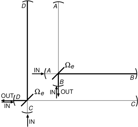
FIG. 4.: Rough sketch of a possible LIGO antenna based on an optical-frequency adaptation of the speed meter.

Figure 4 shows two nearly identical devices, one labeled $11^{\prime}22^{\prime}$, the other labeled $33^{\prime}44^{\prime}$. For the moment ignore $33^{\prime}44^{\prime}$.

Device $11^{\prime}22^{\prime}$ consists of two optical cavities (resonators) $11^{\prime}$ and $22^{\prime}$ that operate at identical resonant frequencies $\omega_{e}$ and are weakly coupled by a mirror with low transmissivity. The mirror causes light to slosh between the two cavities with a sloshing frequency $\Omega=c\sqrt{T}/2d$ where $T$ is the coupling mirror’s very small power transmission coefficient and $d$ is the length of each cavity’s arm. These cavities are the resonators of a speed meter and $d=4$km is the speed meter’s tuning length. By contrast with the microwave speed meter of Fig. 1, which has only one test mass (that coupled to resonator 1), this optical speed meter has (in effect) two test masses, one coupled to each resonator. The reason is that, in order to keep both resonators highly stable, all four mirrors must be suspended as pendula, and the relative displacement $x_{1}$ of mirrors $1^{\prime}$ and $1$ then behaves as a test mass coupled to resonator 1, while the relative displacement $x_{2}$ of $2^{\prime}$ and $2$ behaves as a test mass coupled to resonator 2.

As for the microwave speed meter, we shall read out the classical force (gravity-wave signal) from resonator 1. To guarantee that resonator 1 contains only a velocity signal $dx_{1}/dt$ [or, more precisely, a signal that involves only $dx_{1}/dt$ and its time derivatives] and not any position signal $x_{2}(t)$], it is essential that resonator 2 be unexcited. To achieve this requires, in contrast with the microwave speed meter, that both cavities be driven by input light beams and that the relative amplitudes and phases of those beams be chosen appropriately. Because resonator 2 is unexcited, its mirror motions produce no gravity wave signal, so it does not matter whether it is placed in the same arm as resonator 1, or in the other arm (cf. Fig. 4).

For the configuration in Fig. 4, the two cavities are driven by beams entering their corner mirrors. The end mirrors $1^{\prime}$ and $2^{\prime}$ have the highest possible power reflectivities and the corner mirrors $1$ and $2$ have more modest power reflectivities $R$ designed to produce identical amplitude decay rates $\delta_{e}=c(1-R)/4d$.

As for a conventional LIGO interferometer, so for this speed meter, there is a serious issue of frequency instability for the input light beams. To protect against frequency fluctuations, one could proceed as in a conventional interferometer: Construct two identical speed meters, $11^{\prime}22^{\prime}$ and $33^{\prime}44^{\prime}$ as shown in Fig. 4, with the strongly excited resonators 1 and 3 in the two orthogonal arms of the LIGO vacuum system. Drive the four cavities with phase coherent light beams that are all phase locked to the same master oscillator. Construct the difference of the outputs from 1 and 3 by mixing at a beam splitter, and perform the homodyne detection on that difference. As for a conventional interferometer, such a scheme should provide significant protection against frequency fluctuations.

Although we have not yet carried out a full and detailed analysis of this optical speedmeter, our approximate analyses show that, up to factors of order unity, its performance is described by the same equations as for the microwave speedmeter. It can beat the wide-band SQL by the factors $\xi_{\rm WB}(\omega)$ derived and discussed in Secs. III C, III D and IV.

More specifically, if such an optical speed meter is optimized as in Sec. IV $(\delta_{e}\simeq 2\omega_{0}^{\prime}$, $\Omega\simeq\sqrt{3}\omega_{0}^{\prime}$ where $\omega_{0}^{\prime}$ is the optimal frequency of operation), then to reach the wide-band SQL at $\omega=\omega_{0}^{\prime}$ requires a pump power

$$W=W_{\rm SQL}\simeq 4md^{2}{\omega_{0}^{\prime}}^{4}/\omega_{e}$$ (B1)

[Eq. (104)], and by using a pump power $W$ that exceeds this $W_{\rm SQL}$ and achieving sufficiently low optical losses $\delta_{1}\ll\delta_{e}$, the wide-band SQL can be beat in the vicinity of the optimal frequency $\omega_{0}^{\prime}$ by a factor

$$\xi_{\rm min}=\sqrt{W_{\rm SQL}\over W}\;;\quad\xi_{\rm min}\gtrsim\left({4\delta_{1}\over\delta_{e}}\right)^{1/4}$$ (B2)

[Eqs. (104) and (103)].

Note that the SQL power $W_{\rm SQL}$ corresponds to a stored energy in each resonator $11^{\prime}$ and $33^{\prime}$ given by

$${\cal E}_{\rm SQL}={W_{\rm SQL}\over 2\delta_{e}}\simeq{md^{2}{\omega_{0}^{\prime}}^{3}\over\omega_{e}}\;.$$ (B3)

This is the same stored energy (to within a factor of order unity) as is required to reach the SQL in a conventional LIGO gravitational-wave detector [5]. This stored energy and the corresponding circulating light power $W^{\rm circ}_{\rm SQL}$ in the resonators are uncomfortably large:

$$W^{\rm circ}_{\rm SQL}={{\cal E}_{\rm SQL}\over 2d/c}\sim 900{\rm kW}\;,$$ (B4)

where we have used $m=11$kg, $d=4$km, $\omega_{0}^{\prime}=2\pi\times 100$Hz, and $\omega_{e}=1.8\times 10^{15}{\rm s}^{-1}$ (wavelength $1.06\mu$m), as planned for LIGO [16]. There is hope, in LIGO, of operating at circulating powers of this order [16], but to do so will be extremely challenging. And to beat the SQL by a factor $\xi_{\rm min}$ at the optimal frequency $\omega_{o}^{\prime}$ using the optical speed meter of Fig. 4 would require an even larger circulating power

$$W^{\rm circ}=W_{\rm SQL}^{\rm circ}/\xi_{\rm min}^{2}\;$$ (B5)

[Eqs. (B2)–(B4)]. Moreover, even if such extreme power could be handled in LIGO-III, the resonators’ optical losses might not be much smaller than $\delta_{1}/\delta_{e}\sim 0.01$, which corresponds to a limit on the achievable sensitivity $\xi_{\rm min}\gtrsim(4\delta_{1}/\delta_{e})^{1/4}\simeq 0.4$ (and an increase in event rate for gravitational-wave bursts of $\lesssim 1/0.4^{3}\simeq 15$ over an SQL-limited interferometer).

Although this scheme is rather complex and places extreme demands on the circulating light power and on optical losses, it nevertheless might turn out to be practical. Moreover, it is not significantly more complex or demanding than schemes that have been devised for beating the SQL in LIGO-III by modifying a conventional interferometer’s input and/or output optics [17, 14, 15].

The high power demands of all these schemes leave our research groups dissatisfied and motivate our continuing efforts to find more promising designs that entail much less optical power—schemes that might resemble those described in Refs. [4, 5].

REFERENCES

- [1] V. B. Braginsky and F. Ya. Khalili, Phys. Lett. A 147, 251 (1990).
- [2] V. B. Braginsky and F. Ya. Khalili, Quantum Measurement (Cambridge University Press, Cambridge, 1992).
- [3] V. B. Braginsky and F. Ya. Khalili, Phys. Lett. A 218, 167 (1996).
- [4] V. B. Braginsky, M. L. Gorodetsky and F. Ya. Khalili, Phys. Lett. A 232, 340 (1997).
- [5] V. B. Braginsky, M. L. Gorodetsky and F. Ya. Khalili, Phys. Lett. A 246, 485 (1998).
- [6] These equations should be fairly obvious from the classical theory of microwave networks. For foundations that justify them as quantum mechanical Heisenberg-Picture equations see, e. g., B. Yurke and J. S. Denker, Phys. Rev. A 29, 1419 (1984).
- [7] A. V. Syrtsev and F. Ya. Khalili, JETP, 79, 409 (1994).
- [8] V. B. Braginsky, V. P. Mitrofanov and K. V. Tokmakov, Phys. Lett. A 218, 164 (1996) and unpublished subsequent research.
- [9] V. B. Braginsky, V. S. Ilchenko and K. S. Bagdasarov, Phys. Lett. A, 120, 300 (1987).
- [10] V. B. Braginsky and V. P. Mitrofanov, Systems with Small Dissipation (University of Chicago Press, Chicago, 1985).
- [11] I. A. Bilenko, E. N. Ivanov, M. E. Tobar, D. G. Blair, Phys. Lett. A 211, 136 (1996).
- [12] B. D. Cuthbertson, M. E. Tobar, E. I. Evanov and D. G. Blair, IEEE Trans. Ultrason. Ferroelect. Freq. Control, 45, 1303 (1998).
- [13] T. Suzuki, P. Turner, J. Ferreirinho, D. G. Blair and R. S. Crisp, J. Low Temp. Phys., 58, 37 (1985).
- [14] S. P. Vyatchanin and A. B. Matsko, JETP 77, 218 (1993); S. P. Vyatchanin and E. A. Zubova, Phys. Lett. A 201, 269 (1995); S. P. Vyatchanin and A. B. Matsko, JETP 82, 1007 (1996). S. P. Vyatchanin, Phys. Lett. A, 239, 201 (1998).
- [15] H. J. Kimble, Yu. Levin, A. B. Matsko, K. S. Thorne and S. P. Vyatchanin, paper in preparation.
- [16] R. Weiss et. al., LSC White Paper on Detector Research and Development (LIGO Project Document XXXXX, November 1998).
- [17] W. G. Unruh, in Quantum Optics, Experimental Gravitation, and Measurement Theory, eds. P. Meystre and M. O. Scully, (Plenum, 1982), p. 647.