Is the squeezing of relic gravitational waves produced by inflation detectable?

Abstract

Grishchuk has shown that the stochastic background of gravitational waves produced by an inflationary phase in the early Universe has an unusual property: it is not a stationary Gaussian random process. Due to squeezing, the phases of the different waves are correlated in a deterministic way, arising from the process of parametric amplification that created them. The resulting random process is Gaussian but non-stationary. This provides a unique signature that could in principle distinguish a background created by inflation from stationary stochastic backgrounds created by other types of processes. We address the question: could this signature be observed with a gravitational wave detector? Sadly, the answer appears to be ”no”: an experiment which could distinguish the non-stationary behavior would have to last approximately the age of the Universe at the time of measurement. This rules out direct detection by ground and space based gravitational wave detectors, but not indirect detections via the electromagnetic Cosmic Microwave Background Radiation (CMBR).

I Introduction

The physical processes that took place early in the history of the Universe are well understood at characteristic times $t\gtrsim 1\ \rm sec$, where $t$ denotes proper time after the big bang, in the rest frame of the cosmological fluid. However the processes that took place at times much earlier than this, in what is often called the “very early Universe” are not well understood [1].

A number of theoretical models of the very early Universe have been constructed which differ significantly from each other. In many of these models, phase transitions that take place as the Universe cools (or supercools) play an important role. While it can be difficult to calculate the observational properties of a given model, when this can be done their parameters can often be chosen so that, at late times, the resulting cosmology is consistent with the known observational properties of the present-day Universe. A significant problem is that there is often no way to distinguish between these different models based on strictly objective observational criteria.

One of the most successful models of the very early Universe is the so-called inflationary model. Among the many variations of this basic idea, the most generic and well-studied is the canonical model of “slow-roll inflation” [1, 2]. In this model, the stress-energy tensor of the very early Universe is dominated by a vacuum energy term, which results in an extended epoch of exponential (or near-exponential power-law) expansion. During this epoch, the visible part of the Universe becomes extremely homogeneous and smooth, because the initial fluctuations in the energy density are redshifted into insignificance.

Inflationary models have been extremely successful for several reasons. First, they solve two outstanding problems of modern cosmology, the horizon and flatness problems. Second, they can be described and understood with simple analytical models. Third, they make minimal assumptions. And finally, they make very definite observational predictions about the present-day properties of the Universe. In certain cases, for example in their predictions about the temperature anisotropies in the cosmic background radiation, these inflationary models are in excellent agreement with the observational data [3]. However other models of the early Universe, such as the cosmic string model, are also in good agreement with this data [4].

One of the ways in which different models of the very early Universe can (at least in principle) be distinguished is in the predictions that they make about the stochastic background of gravitational radiation [5, 6]. This is a weak background of gravitational radiation, typically isotropic in its distribution, which is produced at very early times either by the large-scale motions of mass and energy in the cosmological fluid, or by the process of parametric amplification engendered by the expansion of the Universe. Because gravitational forces couple so weakly, this radiation typically evolves free of disturbing influences, and at the present time, its properties provide a picture of the state of the Universe at very early times. To emphasize this point, consider that the present age of the Universe is approximately

$$T_{0}={2\over 3}{H_{0}}^{-1},$$ (1)

where the Hubble expansion rate today is

$$H_{0} = 100\>{\rm km\>sec}^{-1}\>{\rm Mpc}^{-1}\>h_{100}$$ (2)

$$= 3.2\times 10^{-18}{\rm sec}^{-1}\>h_{100}.$$ (3)

Here $h_{100}\approx 0.65$ is a dimensionless parameter. The cosmic microwave background radiation (CMBR) provides us with a picture of the structure of the Universe at a time about $t\approx 100,000\>\text{years}\approx 3\times 10^{12}\>\rm sec$ after the big bang. This should be compared to the present time $T_{0}\approx 3\times 10^{17}\>\rm sec$. On general grounds, the generation of ground-based gravitational wave detectors currently approaching completion might be able to detect a relic background of gravitational waves produced around $t\approx 10^{-22}\>\rm sec$ after the big bang, providing us with a picture of the very early Universe [5].

Of particular interest to us are the two LIGO detectors which will begin engineering shakedown within the next year [7], and the European VIRGO [8] and GEO-600 projects [9]. These ground-based detectors are sensitive in the frequency range from $\sim 10^{1}$ Hz to $\sim 10^{3}$ Hz; long baseline detectors in space such as the proposed LISA [10] project would extend the frequency range downwards by about four orders of magnitude to $\sim 10^{-3}$ Hz. The exciting prospect is to use these instruments to learn something about the physical processes that took place in the very early Universe.

Models of the very early Universe typically predict a relic background of gravitational waves which is stochastic, in the sense that the gravitational strain at any point in the Universe is a non-deterministic function of time which can only be characterized in a probabilistic way. Often, the gravitational strain arises from the sum of a large number of independent processes and so the central limit theorem implies that the resulting random process is Gaussian. In addition, in many models the stochastic background is stationary to a good approximation.

Grishchuk has shown that the stochastic gravitational wave background produced by inflation is Gaussian, but is not stationary [11, 12, 13]. This is because, in inflationary models, the gravitational waves are produced by a process of parametric amplification of vacuum fluctuations, resulting in a squeezed quantum state today. While Grishchuk’s derivation used the language and formalism of quantum optics, the non-stationarity has also been derived using the standard methods of curved spacetime quantum field theory [14, 15].

The non-stationarity of relic waves from inflation is significant for two reasons. First, one calculation indicates that it might make the background easier to detect, because the integrated signal-to-noise ratio can be made to rise faster than the square root of the observation time [16], which is how it would rise for a stationary and Gaussian background [11]. Second, it provides in principle a definite test of inflation: if the squeezing is observed then it provides additional evidence in favor of inflation, and if the background is observed to be not squeezed, then it falsifies the theory.

In this paper we present a detailed analysis of the detectability of the non-stationary statistical properties of relic gravitational waves. We show that, unfortunately, the effect can not be observed in an experiment whose duration is short compared to the age of the Universe at the time of the measurement, which rules out the possibility of measuring the non-stationarity with future ground-based and space-based gravitational wave detectors. The reason is a combination of two effects. First, the statistical properties of the background today vary over a frequency scale $\sim T_{0}^{-1}\sim 10^{-17}\,{\rm Hz}$, and any practical experiment (whose duration is of order a few years or less) will have a frequency resolution which is coarse compared to $T_{0}^{-1}$. Second, there is an inherent and unavoidable limitation in the accuracy of our measurement of statistical properties of a random process, due to the stochastic nature of the random process. This limitation is analogous to what is called “cosmic variance” in measurements of CMBR anisotropies.

We also show that even in a gedanken experiment lasting long enough to distinguish between the stationary and non-stationary background, there does not appear to be any way to exploit the latter to make the integrated signal to noise grow faster than the square root of the integration time [16].

We note in passing that it may be possible in the future to probe the squeezed nature of relic gravitons, albeit indirectly. Sakharov oscillations in the angular spectrum of temperature fluctuations in the CMBR are produced by a combination of tensor perturbations (gravitational waves) and scalar perturbations. The existence of these Sakharov oscillations is directly related to the squeezed nature of the tensor and scalar perturbations [17]. If it is possible in the future to disentangle the scalar and tensor contributions to the CMBR anisotropies (perhaps using polarization information [18]), it may be possible to confirm that the gravitational waves are indeed squeezed. However it appears that will not be possible with the upcoming MAP and PLANCK experiments [19]. Note that the possibility of such a measurement is consistent with our analysis, since CMBR photons effectively “measure” the gravitational perturbations over a time larger than or of order the age of the Universe at recombination.

The paper is organized as follows. In Appendix A we review the predictions of general inflationary models for the statistical properties of relic gravitational waves. In Sec. II A we extract the cogent features of those predictions in the context of a simple model problem, a scalar field in $1+1$ dimensions, and describe the differences between stationary and squeezed random processes in this context. In the remainder of Sec. II and in Appendices B and C we analyze in detail measurements that take place at one point in space. We show that in order to distinguish between the stationary and squeezed processes in this context, a necessary but in general not sufficient condition is that individual modes need to be resolved with a precision that can only be achieved with an experiment lasting a substantial fraction of the age of the Universe. The arguments do not rely on any specific inflationary model. Similar conclusions were reached in work by Polarski and Starobinsky (page 389 of [14]).

In Sec. III we present a more detailed analysis that relaxes the assumptions of our simplified analysis of Sec. II. We consider an explicit model of slow-roll inflation, and calculate the two-point correlation function $C(t,t^{\prime})=\langle h_{1}(t)h_{2}(t^{\prime})\rangle$ of detector strain at two different sites. This is the quantity that will be measured in the upcoming generation of experiments in searches for a stochastic background [5, 6]. We are able to obtain and confirm the main results of Ref. [11]: due to the squeezing, non-stationary terms (not functions of $t-t^{\prime}$) arise in $C(t,t^{\prime})$. Unfortunately we also show that the non-stationary terms are averaged away in any observation which is short compared to $T_{0}$. In addition, from the explicit expression of the correlation function it can be seen that the integrated signal to noise after optimum filtering should grow with the square root of the integration time [16] and not faster.

Of course it is a dangerous game to claim that something is not possible. The history of physics is full of “no-go” theorems that have been circumvented by clever experiments. But our work does show that identifying the squeezed nature of the gravitational waves produced in an inflationary Universe is probably not possible with ground and space based gravitational wave detectors.

II Simplified Detectability analysis

A Stationary and Squeezed random processes

The statistical properties of relic gravitational waves, as predicted by inflationary models, are summarized in Appendix A. In this section we present an analysis of the detectability of the non-stationarity in the following simplified context. Consider a flat $1+1$-dimensional spacetime with topology $R\times S^{1}$, with spatial circumference $2\pi L$, and metric

$$ds^{2}=L^{2}(-dt^{2}+dx^{2}),$$ (4)

where the periodic spatial coordinate $x\in[0,2\pi)$ and $t$ is now a dimensionless time coordinate. We assume a compact spatial topology for technical convenience only; the discrete mode normalization is simpler than the corresponding continuum normalization. As a model of gravitational wave perturbations, consider solutions to the scalar massless wave equation

$$\left(-{\partial^{2}\over\partial t^{2}}+{\partial^{2}\over\partial x^{2}}\right)h=0$$ (5)

in the spacetime (4). The periodic nature of the spatial sections means that solutions to the wave equation are periodic in time, and have discrete frequencies. The frequencies are separated by $\Delta f=1/(2\pi L)$.

The analog in this context of a stationary, Gaussian stochastic background (the naive prediction of inflationary models) is a scalar field of the form :

$$h_{\rm stationary}(t,x)=\sum_{n=-\infty}^{\infty}r_{n}\cos(|n|t+nx+\phi_{n}).$$ (6)

This solution to the wave equation (5) describes a particular type of stochastic random process. It can can be obtained from Eq. (A9) below by dropping the second term, by restricting the unit vector ${\bf n}$ to have two allowed values, and by using a discrete instead of a continuous mode normalization. Here the quantities $r_{n}$ and $\phi_{n}$ for $n=\pm 1,\pm 2,\ldots$ are random variables whose statistical properties are given by

$$r_{n}e^{i\phi_{n}}=x_{n}+iy_{n},$$ (7)

where $x_{n}$ and $y_{n}$ are independent, zero-mean Gaussian random variables with $\langle x_{n}^{2}\rangle=\langle y_{n}^{2}\rangle=\sigma_{n}^{2}/2$. The variance $\sigma_{n}$ can depend on $n$ in an arbitrary way, but typically in inflationary models $\sigma_{n}$ has a power law dependence over a broad range of wavenumbers or frequencies: $\sigma_{n}=\alpha|n|^{\beta}$ for some constants $\alpha$ and $\beta$. It follows from Eq. (7) that the $r_{n}$’s and $\phi_{n}$’s are all independent, that the $r_{n}$’s are Rayleigh distributed, and that the $\phi_{n}$’s are uniformly distributed over the interval $[0,2\pi)$.

What Grishchuk has shown is that inflation leads to a slightly different random process, one which to very good approximation can be written as

$$h_{\rm squeezed}(t,x)=\sum_{n=-\infty}^{\infty}\sqrt{2}\,r_{n}\cos(nt)\cos(nx+\phi_{n}),$$ (8)

where the $r_{n}$’s and $\phi_{n}$’s are distributed as before. The factor of $\sqrt{2}$ ensures that the processes $h_{\rm stationary}$ and $h_{\rm squeezed}$ have the same time-averaged energy density. Note that the stationary random process (6) is invariant under changes $t\to t-\Delta t$ of the origin of the time coordinate, but that the squeezed random process (8) is not. In Sec. III and Appendix A we show that in inflation models, the simple form (8) is achieved when one chooses a particular origin for the conformal time coordinate during the inflationary epoch. Again, Eq. (8) can be obtained from Eq. (A9) below by restricting the unit vector ${\bf n}$ to have two allowed values, by using a discrete instead of a continuous mode normalization, by taking $\chi(k)=0$, and by specializing the the limit of large squeezing $|\beta_{k}|\gg 1$.

Note that we can rewrite the squeezed random process (8) as

$$h_{\rm squeezed}(t,x)=\sum_{n=1}^{\infty}\sqrt{2}\,{\bar{r}}_{n}\cos(nt)\cos(nx+{\bar{\phi}}_{n}),$$ (9)

where now the sum is only over positive values of $n$, and

$${\bar{r}}_{n}e^{i{\bar{\phi}}_{n}}=r_{n}e^{i\phi_{n}}+r_{-n}e^{-i\phi_{-n}}.$$ (10)

It follows from Eqs. (7) and (10) that

$${\bar{r}}_{n}e^{i{\bar{\phi}}_{n}}={\bar{x}}_{n}+i{\bar{y}}_{n}$$ (11)

where ${\bar{x}}_{n}$ and ${\bar{y}}_{n}$ are independent, zero-mean Gaussian random variables with $\langle{\bar{x}}_{n}^{2}\rangle=\langle{\bar{y}}_{n}^{2}\rangle=\sigma_{n}^{2}$. Thus the squeezed random process can be described by half as many independent random variables as the stationary one. We also note that a solution to the two-dimensional wave equation is completely specified by $h$ and $\dot{h}$ at some instant in time, where overdot denotes $\partial/\partial t$. Thus, given the two functions $f(x)=h_{\rm stationary}(0,x)$ and $g(x)=\dot{h}_{\rm stationary}(0,x)$ one can uniquely determine $r_{n}$ and $\phi_{n}$. The function $h_{\rm squeezed}$ has only half the number of degrees of freedom, and it is easy to show that it is a solution to the wave equation determined entirely by $f(x)=h_{\rm squeezed}(0,x)$.

Below we shall be concerned with observations at a fixed point in space, which without loss of generality we can take to be the point $x=0$. The two random processes evaluated at $x=0$ yield

$$h_{\rm stationary}(t,0) = \sum_{n=1}^{\infty}\left[{\hat{x}}_{n}\cos(nt)+{\hat{y}}_{n}\sin(nt)\right]$$ (12)

$$h_{\rm squeezed}(t,0) = \sum_{n=1}^{\infty}\sqrt{2}\,{\bar{x}}_{n}\cos(nt),$$ (13)

where

$${\hat{x}} = x_{n}+x_{-n}$$ (14)

$$\mbox{}{\hat{y}}_{n} = -y_{n}+y_{-n}.$$ (15)

From Eqs. (10), (11) and (15) the random variables ${\bar{x}}_{n}$, ${\bar{y}}_{n}$, ${\hat{x}}_{n}$ and ${\hat{y}}_{n}$ are all independent, zero mean Gaussians with variance $\sigma_{n}^{2}$.

Another convenient way of representing the processes $h_{\rm stationary}(t,0)$ and $h_{\rm squeezed}(t,0)$ is to go from the time domain representation of these fields to their frequency domain representation, through the Fourier transformation equations. The signals of Eqs. (12) can be expressed as a superposition of a discrete infinite set of cosine functions:

$$h(t,0)=\sum_{n=1}^{\infty}R_{n}\cos(nt+\theta_{n})={\rm Re}\sum_{n=1}^{\infty}R_{n}{\rm e}^{i(nt+\theta_{n})},$$ (16)

defined, for every frequency $n$, by the Fourier amplitudes $R_{n}$ and phases $\theta_{n}$. These are what we shall refer to as “the Universe modes”. The relations between the coefficients appearing in Eq. (16) and those in Eq. (12) are, for the stationary case:

$$R_{n} = \sqrt{{\hat{x}}_{n}^{2}+{\hat{y}}_{n}^{2}}$$ (17)

$$\theta_{n} = \arg\big{[}{\hat{x}}_{n}+i{\hat{y}}_{n}\big{]},$$ (18)

where the range of $\arg$ is $[0,2\pi)$, and for the squeezed case:

$$R_{n} = \sqrt{2}\,|{\bar{x}}_{n}|$$ (19)

$$\theta_{n} = \cases{0~{}~{}~{}~{}{\rm{if}}~{}~{}~{}~{}{\bar{x}}_{n}>0\cr\pi~{}~{}~{}~{}{\rm{if}}~{}~{}~{}~{}{\bar{x}}_{n}<0}.$$ (20)

It is convenient to think of each mode as a vector in the complex plane having length $R_{n}$ and phase $\theta_{n}$. This allows one to perform calculations using complex exponentials - which is easier - and also to have a useful pictorial representation of what the field is. In the stationary case, it can be seen from Eq. (17) that the phases $\theta_{n}$ are uniformly distributed on the interval $[0,2\pi)$. In the squeezed case, instead, the phases can only have two values, namely $0$ or $\pi$. This means that whereas the mode vectors for the stationary case are randomly pointing in any direction in the complex plane, in the squeezed case they all lie on the real axis (see Fig. 2). This is the origin of the name “squeezed”. Also the distribution of the amplitudes $R_{n}$ is quite different in the two cases, as can be seen from Fig. 1.

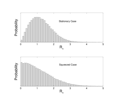
FIG. 1.: Histogram of amplitudes $R_{n}$ for the stationary (upper panel) and squeezed (lower panel) cases for a mode with $\sigma_{n}^{2}=1$, from a total of $10^{5}$ points.

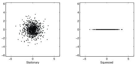
FIG. 2.: The distribution of the complex vectors of a mode with $\sigma_{n}^{2}=1$ in the stationary and in the squeezed case (from a total of $10^{3}$ points).

B Distinguishing between the two random processes in principle

The question that must be addressed is this: what experiment can we perform that will in practice be able to distinguish between these two different random processes, (6) and (8)? In other words, can we construct some observational statistic that will enable us to determine with high confidence which of these two random processes is present, given a single realization?

To appreciate this issue a bit more clearly, consider that both $h_{\rm stationary}$ and $h_{\rm squeezed}$ are solutions to the two-dimensional wave equation (5). This fact can help us to compare the properties of these two random processes. Roughly speaking, the standard process $h_{\rm stationary}$ is a sum of left and right moving waves with arbitrary amplitudes and phases:

$$h_{\rm stationary}(t,x) = \sum_{n=1}^{\infty}\bigg{\{}r_{n}\cos[n(t+x)+\phi_{n}]$$ (22)

$$+r_{-n}\cos[n(t-x)+\phi_{-n}]\bigg{\}}.$$

In contrast to this, the Grishchuk process $h_{\rm squeezed}$ is a sum of standing waves

$$h_{\rm squeezed}(t,x) = \sum_{n=1}^{\infty}{{\bar{r}}_{n}\over\sqrt{2}}\bigg{\{}\cos[n(t+x)+{\bar{\phi}}_{n}]$$ (24)

$$+\cos[n(t-x)-{\bar{\phi}}_{n}]\bigg{\}},$$

for which the left and right moving waves have equal amplitudes and correlated phases.

Now suppose that we ask the following question: could we distinguish between these two possible forms of $h(t,x)$ based on unrestricted observations? The answer is obviously “yes”. We would simply observe the evolution and see if there was a standing wave pattern or not: a standing-wave pattern would imply $h_{\rm squeezed}$, anything else would falsify inflation.

A slightly more difficult question is the following: suppose that instead we can only observe the function at a single point in space: $h(t,x=0)$. Again, could we distinguish between these possibilities? Once again, the answer is clearly yes. By observing the process $h(t,0)$ for $0\leq t<2\pi$ and Fourier transforming, we can recover the complex coefficients $R_{n}\exp[i\theta_{n}]$ in the expansion (16). If any of these coefficients have non-zero imaginary parts, then the process must be stationary rather than squeezed, by Eqs. (19).

However, our assumption of spatial periodicity (which ensures the periodicity in time) is just a computational device – essentially an infrared cutoff. We must at the end of our calculation let this cutoff go to infinity to obtain physical results. In this limit, the measurement discussed above corresponds to a measurement of the random process over an infinite time, since the proper-time duration of the measurement is $2\pi L$ which diverges as $L\to\infty$. So, the conclusion so far is that it would be possible to distinguish between the stationary and squeezed processes, provided that one had complete knowledge of the function $h(t,x=0)$ over the entire time history of the Universe.

C Distinguishing between the two random processes in practice

Consider now realistic measurements of the stochastic background. Such measurements will be subject to three key constraints:

• The function $h(t,x=0)$ can only be observed over a limited range of time $T_{s}\leq\tau\leq T_{s}+T_{\rm obs}$, where $\tau=Lt$ is proper time, the starting time $T_{s}$ is essentially the age of the Universe $T_{0}$, and the duration $T_{\rm obs}$ of the measurement is much smaller than $T_{0}$. In practice the longest possible observation times will be $T_{\rm obs}\approx 1\>{\rm year}\>\approx 3\times 10^{7}\>{\rm sec}$.

• The detectors available to us can not observe all of the modes, but just a (fairly narrow) range in frequency $f\in[f_{0},f_{0}+\Delta f]$ where typically $f_{0}\sim\Delta f\sim 100\>\rm Hz$ for ground based detectors, and $f_{0}\sim 10^{-4}\,{\rm Hz}$, $\Delta f\sim 10^{-2}\,{\rm Hz}$ for space based detectors.

• The detectors that measure $h(t,0)$ are intrinsically noisy, limiting the accuracy of our measurements.

We now show that the short observation time constraint ($T_{\rm obs}\ll T_{s}$ ) alone makes it impossible to distinguish between stationary and squeezed. In order to show this, we will derive the relation between the Universe modes and the observed modes that we actually measure. We will show that the latter are a weighted superposition of the former ones, and that the process of superposition makes it impossible to trace back the phase coherence of the squeezed case.

Our analysis in this section will be limited to observations made at a single point in space. This assumption is of course not realistic, as realistic measurements will involve cross-correlating between spatially separated detectors. We present a more complete analysis which relaxes this restriction in Sec. III below.

We start by making a convenient change in our representation of the stochastic background. So far, we have treated the stochastic background as a continuous function of $t$ – a random process $h(t,0)$ – whose frequency representation is discrete due to the assumed infrared cutoff (spatial periodicity). We now switch to a discrete representation of the stochastic background in the time domain, by modeling the background as a set of $N$ numbers

$$h_{j}=h(j\Delta t),$$ (25)

for $0\leq j\leq N-1$ where $N\Delta t=2\pi$. Thus, we have effectively imposed an ultraviolet cutoff. At the end of our calculation we can let $\Delta t\to 0$ and obtain a result that is independent of $\Delta t$ [cf. Eq. (B22) below]. The discrete Fourier transform (DFT) of the sequence (25) is given by the relation

$$\tilde{h}_{j}=\sum_{k=0}^{N-1}e^{2\pi\imath{jk\over N}}h_{k},$$ (26)

whose inverse is

$${h_{k}}={1\over N}\sum_{j=0}^{N-1}e^{-2\pi\imath{jk\over N}}\tilde{h}_{j}.$$ (27)

We will also assume that the statistical properties of the quantities ${\tilde{h}}_{j}$ are the same as those of the quantities $R_{n}\exp[i\theta_{n}]$ of Eq. (16) above, namely

$$\langle({\rm Re}\,{\tilde{h}}_{j})^{2}\rangle = (1+\varepsilon)\sigma_{j}^{2}$$ (28)

$$\mbox{}\langle({\rm Im}\,{\tilde{h}}_{j})^{2}\rangle = (1-\varepsilon)\sigma_{j}^{2},$$ (29)

where $\varepsilon=0$ in the stationary case and $\varepsilon=1$ in the squeezed case. Equation (29) will not be exactly true but will be true to an adequate approximation.

Lets now take our measurement to consist of the quantities

$$H_{A}=h_{s+A}$$ (30)

for $0\leq A\leq M-1$, where $s$ and $M$ are fixed integers with $0<s<N$ and $0<M\leq N-s$. Thus, the starting proper-time of the measurement is $T_{s}=sL\Delta t$ and the duration of the measurement is $T_{\rm obs}=ML\Delta t$. Henceforth capital Roman indices ($A$, $B$, $C$, $\ldots$) will be measurement indices that run over $0,1,\ldots,M-1$, while lower case Roman indices ($i,j,k,\ldots$) will run over $0,1,\ldots,N-1$. The DFT

$${\tilde{H}}_{A}=\sum_{B=0}^{M-1}e^{2\pi\imath{AB\over M}}H_{B}$$ (31)

of the quantities (30) define the amplitudes of what we will call the measured modes.

We can compute the relation between the measured mode amplitudes (31) and the Universe mode amplitudes (26) by inserting Eqs. (27) and (30) into Eq. (31), which gives

$$\tilde{H}_{A}=\sum_{p=0}^{N-1}W_{Ap}\tilde{h}_{p}.$$ (32)

Here the coefficients $W_{Ap}$ are given by

$$W_{Ap} = {1\over N}\,e^{-2\pi\imath{ps\over N}}\,\sum_{B=0}^{M-1}\,e^{2\pi\imath({A\over M}-{p\over N})B}$$ (33)

$$= \displaystyle{1\over N}\ e^{-2\pi\imath{ps\over N}}\,\left[\displaystyle{1-e^{-2\pi\imath{pM\over N}}\over 1-e^{2\pi\imath({A\over M}-{p\over N})}}\right].$$ (34)

Equations (32) and (34) say that the complex vectors $\tilde{H}_{A}$ (amplitudes of the observed modes) that define the DFT from the shorter time baseline (30) are a weighted sum of the vectors $\tilde{h}_{p}$ (amplitudes of the Universe modes) that define the DFT from the longer time baseline (25). The weights are complex numbers whose magnitudes depend only on the distance in frequency between $A$ and $p$. In order to make this statement clearer, let us take a closer look at $W_{Ap}$ and introduce a new index variable

$$A^{\prime}=A{M\over N}.$$ (35)

This variable can take values from $0$ to $M-1$, as does the index $A$, but is not an integer. It measures the position of the points $p$ on the $A$ axis. In terms of this new variable the weights take the form

$$W_{AA^{\prime}}=\displaystyle{1\over N}\ e^{-2\imath\pi A^{\prime}s/M}\ e^{\imath\pi(A-A^{\prime})(1-1/M)}\ {\sin\left[\pi(A-A^{\prime})\right]\over\sin\left[{\pi\over M}(A-A^{\prime})\right]}$$ (36)

Note that when $A^{\prime}$ is an integer, we have $W_{AA^{\prime}}=W_{A^{\prime}A}^{*}$, which is necessary since the random sequences $h_{j}$ and $H_{A}$ are real. Also we can write

$$W_{AA^{\prime}}={M\over N}f_{M}(|A-A^{\prime}|)e^{i\varphi_{AA^{\prime}}}$$ (37)

with

$$f_{M}(x)=\displaystyle{\sin{\pi x}\over M\sin{{\pi\over M}x}},$$ (38)

which shows that the absolute values of the weights depend only on the distance $(A-A^{\prime})$ between $A$ and $p$. Figure 3 shows the magnitudes $|W_{AA^{\prime}}|$ of the weights for the case $M=10$, $N=100$. This figure makes it clear that the Universe modes that contribute the most to a given observed mode, in the sum (32), are those which are nearest to it. It also shows that for any measured mode $A$, the amplitudes of the Universe modes to the right of $A$ (i.e. modes with $A^{\prime}>A$) are weighted in the same way as the modes to its left ($A^{\prime}<A$), which follows from $|W_{A\,A+\Delta A}|=|W_{A\,A-\Delta A}|$.

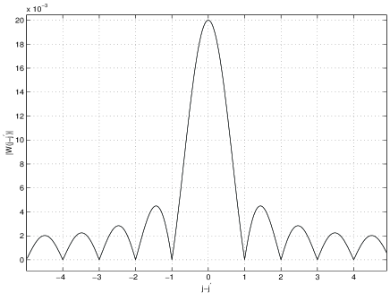
FIG. 3.: This plot shows the behavior of $|W_{AA^{\prime}}|$ as a function of $A-A^{\prime}$ for the case $M=10$, $N=500$. The maximum value is ${M\over N}={10\over 500}$.

The crucial property of the weighting factors $W_{AA^{\prime}}$ is that they contain oscillations on two different frequency scales. First, there is above-discussed oscillation in the magnitude $|W_{AA^{\prime}}|$ with characteristic frequency scale $\sim T_{\rm obs}^{-1}$. Second, there is in addition a variation in the phase of $W_{AA^{\prime}}$, encoded in the factor $\exp[-2\pi\imath A^{\prime}s/M]$ in Eq. (36), with characteristic frequency scale $\sim T_{s}^{-1}$.

We can now give the key argument. Consider a particular measured mode amplitude ${\tilde{H}}_{A}$, which corresponds to a physical frequency $f_{A}=A/(ML\Delta t)$. This mode amplitude results from a vectorial sum (32) of Universe mode amplitudes ${\tilde{h}}_{j}$. The Universe modes ${\tilde{h}}_{j=NA^{\prime}/M}$ which contribute significantly to ${\tilde{H}}_{A}$ all lie with a frequency interval around $f_{A}$ of width $\sim T_{\rm obs}^{-1}$, because of the oscillations in $|W_{AA^{\prime}}|$. Now, if the weighting factors $W_{AA^{\prime}}$ were all real in this frequency interval, then since in the squeezed case the Universe mode amplitudes ${\tilde{h}}_{j}$ are all real, then the resulting measured mode amplitude ${\tilde{H}}_{A}$ obtained from the sum (32) would also be real. Hence, the observed mode amplitude would share with the original Universe mode amplitudes that property that its phase is constrained to be $0$ or $\pi$, and so the squeezing would be easily observable.

Thus, we see that the crucial point is the extent to which the weighting factors can be treated as real in the frequency interval of width $\sim T_{\rm obs}^{-1}$ around the central frequency $f_{A}$. Consider first the short-measurement regime $T_{\rm obs}\ll T_{s}$. In this regime, the phase of $W_{AA^{\prime}}$ winds around between $0$ and $2\pi$ roughly $T_{s}/T_{\rm obs}\gg 1$ times in the frequency interval, due to the factor $\exp[-2\pi\imath A^{\prime}s/M]$ in Eq. (36), and so cannot be treated as real. In this case the observed mode ${\tilde{H}}_{A}$ has a phase that is very nearly uniformly distributed over $[0,2\pi)$; the vectorial sum (32) almost completely erases the peculiar phase behavior of the non-stationary process. This is in part due to the fact that the vectorial sum entangles phase and amplitude information and that the amplitudes of the Universe modes (although not the phases) are stochastic. In Appendix B below we demonstrate this by deriving the distributions of the phase and amplitude of the observed amplitude ${\tilde{H}}_{A}$.

So far, we have argued that the effect of the squeezing on the statistical properties of each observed mode ${\tilde{H}}_{A}$ is very small in the regime $T_{\rm obs}\ll T_{s}$. This gives the essential reason why the squeezing is not observable. However, we still need to close two loopholes in the argument. First, we have not yet shown that the effect of squeezing is unobservable, as we have not addressed the question of how accurately the statistical properties of each mode can be measured. In the case of the CMBR, for example, the anisotropies are smaller than the homogeneous background CMBR by a factor of $10^{5}$, yet those anisotropies are still observable and carry a great deal of information. We need to show that the intrinsic limitations in the possible accuracy of measurement of the statistical properties of each mode (“cosmic variance”) are larger than the effect of squeezing on each mode. Second, it is insufficient to perform an analysis that focuses on each individual measured mode ${\tilde{H}}_{A}$ one at a time, as the individual measured modes are not statistically independent, and we need to show that squeezing cannot be observed in any measurement that combines information from all the measured modes [20]. These two concerns are addressed and resolved in Appendix B, where we demonstrate that the effect of squeezing is indeed not observable.

For completeness, we now consider the long measurement regime $T_{\rm obs}\gg T_{s}$, although as explained in the Introduction this regime cannot be realized in practice. In this regime, the oscillation in the phase of $W_{AA^{\prime}}$ due to the factor $\exp[-2\pi\imath A^{\prime}s/M]$ in Eq. (36) is negligible. There is a phase oscillation due to the factor $\exp[\pi\imath(A-A^{\prime})(1-1/M)]$ in Eq. (36), which gives a total change of phase of order unity over the frequency interval. The resulting observed mode amplitude ${\tilde{H}}_{A}$ is thus not constrained to be real. It turns out that the probability distribution for its phase ${\rm Arg}{\tilde{H}}_{A}$ is exactly uniform in the case when the spectrum is white, i.e., when $\sigma_{j}=$ const. When the spectrum is colored, the detectability of the squeezing depends on how large $T_{s}$ is compared to a correlation time determined by the spectrum $\sigma_{j}$ (see Appendix B).

III Two-detector correlation experiments

A Introduction

In this section we extend the analysis of Sec. II of the detectability of the non-stationarity to incorporate a number of complicating effects, including the effect of having measurements at more than one point in space. We restrict attention in this section to the realistic case of short observations, $T_{\rm obs}\ll T_{s}$.

The standard method which will be used to detect a stochastic gravitational-wave background is based on correlating two widely-separated detectors. In the standard treatments of this technique, one considers a stochastic background which is stationary and Gaussian. In this case it is easy to show that the integrated two-detector correlation arising from the stochastic background is proportional to the integration time, whereas the terms arising from the (assumed uncorrelated) detector noise are proportional to the square root [16] of the integration time.

As stressed by Grishchuk, the stochastic background produced by an inflationary epoch in the early Universe is in a squeezed quantum state produced by the period of rapid expansion. The statistical properties of this state are Gaussian, but not stationary. Unfortunately the non-stationary behavior does not make the stochastic background produced by inflation easier to observe than a similar background which is stationary and Gaussian. We show this in Sec. III B below by deriving an expression for the correlation function for the detector strains at two separated sites. We show that, in contrast with the correlation function for a stationary Gaussian background (which depends only upon $t-t^{\prime}$), the squeezed nature of the inflationary background gives rise to an extra term in the correlation function. This extra term explicitly manifests the non-stationary nature of the squeezed state: it is not a function of $t-t^{\prime}$ alone. Thus Grishchuk is entirely correct that the squeezed quantum state has different properties than a stationary and Gaussian background. However we show that observing this extra non-stationary term requires a frequency resolution of order $10^{-17}$ Hz. Such incredible frequency resolution is only obtainable in a gedanken experiment lasting as long as the present-day age of the Universe.

The calculation in this Section makes frequent use of results from two references. The first reference examines the gravitational waves produced by an inflationary epoch in the early Universe [22], and calculates the correlation function of the temperature anisotropies that they induce in the CBR. The frequency range of the waves influencing the observable part of the CBR anisotropy is between $10^{-18}\>\text{Hz}$ and $10^{-16}\>\text{Hz}$ today. But the methods of Ref. [22] can also be applied (as we do here) to calculate the properties of the waves at much higher frequencies: the $10^{-3}\>\text{Hz}$ relevant to space-based or the $10^{2}\>\text{Hz}$ relevant to earth-based gravitational-wave detectors. The second reference that we make use of is a review article on how correlation techniques may be used to detect a stochastic background [6]. A reader wishing to follow our calculations in detail is advised to have copies of these two papers in hand.

The calculation done in this Section is for an explicit model of slow-roll inflation, in the limit that the resulting spectrum is “flat” and not tilted. After completing the explicit calculation of the correlation function, it is straightforward to show that in more general inflationary models, which produce a “tilted” spectrum, the same general conclusion holds: the non-stationary behavior can not be observed in any practical experiment.

B Calculation of the correlation function $C(t,t^{\prime})$

The most direct way to understand how the squeezing produced in an inflationary model affects the correlation between separated detectors is to examine the two-point correlation function for the gravitational wave strain $h$ at two detector sites. This is defined by:

$$C(t,t^{\prime})=\langle h_{1}(t)h_{2}(t^{\prime})\rangle$$ (39)

where the subscripts $1$ and $2$ refer to the detector sites, and $t$ and $t^{\prime}$ denote the time at these sites. The angle brackets can be given two possible (equivalent) meanings. They can denote the average over a statistical ensemble of many different inflationary Universes, each starting from somewhat different initial conditions, but made statistically similar by a long period of exponential inflation. Equivalently, they can denote the expectation value in a quantum state that is a good approximation to the present-day state of the Universe.

The detector strains are given in terms of the metric perturbations of a Friedman-Robertson-Walker (FRW) cosmological model. Denoting the space-time metric by

$$ds^{2}=a^{2}(\eta)\left(-d\eta^{2}+(\delta_{ab}+h_{ab})dx^{a}dx^{b}\right)$$ (40)

the strain at site $i$ is given by:

$$h_{i}(t)={1\over 2}h_{ab}(t,{\bf x}_{i})(\hat{X}_{i}^{a}\hat{X}_{i}^{b}-\hat{Y}_{i}^{a}\hat{Y}_{i}^{b})$$ (41)

where ${\bf x}_{i}$ is the spatial location of the $i$-th site and $\hat{X}_{i}^{a}$ and $\hat{Y}_{i}^{a}$ are unit-length spatial vectors (with respect to the metric $\delta_{ab}$) along the directions of the orthogonal detector arms at site $i$. Our model of the Universe is specified via the cosmological scale factor $a(\eta)$ given as a function of conformal time $\eta$ by Eq. (47). Note that we frequently use cosmological time $t$ rather than conformal time $\eta$ as a coordinate; they are related by $dt=a(\eta)d\eta$.

To compute the correlation function, we need an expression for the metric perturbation $h_{ab}$. This quantity is not deterministic. In classical calculations, it may be treated as a real stochastic random variable with certain statistical properties. For inflationary cosmological models, a slightly different approach is useful, in which $h_{ab}$ is replaced by the field operator $\bar{h}_{ab}$ of the linearized gravitational field. To see why this is both simple and useful, it is helpful to briefly review the fundamental mechanism through which inflationary models erase the effects of the conditions present before the inflation begins and give rise to a spatially flat and homogeneous Universe today.

In inflationary models, the Universe undergoes a period of (nearly) exponential expansion of the scale factor $a$. During this period, the energy-density of any matter or radiation is red-shifted away exponentially quickly. For massless particles, the energy of a particle is proportional to $a^{-1}$ and hence the energy-density in massless particles redshifts as $a^{-4}$. For massive particles, any kinetic energy is quickly red-shifted away, leaving only the rest-mass behind. This energy is diluted by the expansion of the spatial three-volume, so that the energy-density of massive particles redshifts away as $a^{-3}$. What is left behind after the period of exponential inflation is just the vacuum energy associated with the cosmological constant; it is the dominant form of energy at the end of an inflationary epoch.

The perturbations away from absolute uniformity in inflationary models are dominated by the effects of the zero-point vacuum fluctuations of the fields at the start of inflation [23]. Twenty five years ago Grishchuk showed that during the subsequent expansion of the Universe, the quantum zero-point fluctuations of the gravitational field modes are parametrically amplified [24]. This prediction has been subsequently confirmed in many different ways, and the process of parametric amplification, which applies to both scalar and tensor perturbations, is one explanation of how the early Universe can generate a spectrum of perturbations.

The above discussion, combined with Eqs. (39) and (41), implies that the correlation function today is well approximated by the vacuum expectation value

$$C(t,t^{\prime}) = {1\over 8}\langle 0|{\bar{h}}_{ab}(t,{\bf x}_{1}){\bar{h}}_{cd}(t^{\prime},{\bf x}_{2})+{\bar{h}}_{cd}(t^{\prime},{\bf x}_{2}){\bar{h}}_{ab}(t,{\bf x}_{1})|0\rangle$$ (43)

$$(\hat{X}_{1}^{a}\hat{X}_{1}^{b}-\hat{Y}_{1}^{a}\hat{Y}_{1}^{b})(\hat{X}_{2}^{c}\hat{X}_{2}^{d}-\hat{Y}_{2}^{c}\hat{Y}_{2}^{d}),$$

where $|0\rangle$ is the (unique Hadamard de Sitter-invariant) quantum vacuum state of the inflationary Universe [25], and $\bar{h}_{ab}$ is the Hermitian field operator of the linearized gravitational field.

The correlation function (43) can be calculated exactly, but since space and ground based detectors will only be sensitive to gravitational waves in the frequency range $f\in[10^{-3},10^{3}]$ Hz, a number of simplifying approximations can be made. We do this by approximating the field operator within this frequency range. In general, the field operator is given by Ref. [22] as

$$\bar{h}_{ab}(\eta,{\bf x}) = \int d^{3}k\>\bigg{(}e^{i{\bf k}\cdot{\bf x}}\big{[}e_{ab}({\bf k})\phi_{R}(\eta,k)\bar{a}_{R}({\bf k})$$ (45)

$$+e^{*}_{ab}({\bf k})\phi_{L}(\eta,k)\bar{a}_{L}({\bf k})\big{]}+{\rm h.c.}\bigg{)},$$

where ${\rm h.c.}$ means Hermitian conjugate. This is a sum over wavevectors (labeled by $\bf k$) of left- and right-circular polarization tensors $e_{ab}$ and $e^{*}_{ab}$ and wavefunctions $\phi_{L,R}(\eta,k)\exp(\imath\bf k\cdot\bf x)$. To approximate the field operator we need to relate present-day frequency $f$ to $k=|{\bf k}|=\sqrt{k_{a}k^{a}}$. Since $\bf k$ always appears in the form $\exp(\imath\bf k\cdot\bf x)$, from the form of the metric (40) one can see that the frequency $f$ today is related to $k$ by

$$f={k\over 2\pi a(\eta_{0})}.$$ (46)

We will now express this relationship between $f$ and $k$ in terms of the present-day Hubble expansion rate $H_{0}$, which will yield Eq. (52). This leads to relations (54) needed to approximate the field operator (45) and to evaluate the two-point correlation function (43) in the frequency range of interest.

The inflationary cosmological model is defined by the scale factor $a(\eta)$ in Eq. (4.1) of Ref. [22]:

$$a(\eta)=\left\{\begin{array}[]{lll}\big{(}2-{\eta\over{\eta_{1}}}\big{)}^{-1}a({\eta_{1}})&-\infty<\eta<{\eta_{1}}&{\rm de\ Sitter,}\\ &&\\ {\eta\over{\eta_{1}}}a({\eta_{1}})&{\eta_{1}}<\eta<{\eta_{2}}&{\rm radiation,}\\ &&\\ {1\over 4}\big{(}1+{\eta\over{\eta_{2}}}\big{)}^{2}{{\eta_{2}}\over{\eta_{1}}}a({\eta_{1}})&{\eta_{2}}<\eta&{\rm matter}.\end{array}\right.$$ (47)

This scale factor describes three epochs: a de Sitter inflationary phase, followed by a radiation-dominated and then a matter-dominated phase. Letting $t$ be the cosmological time defined by $dt=a(\eta)d\eta$, the Hubble constant today is given by:

$$H_{0} = \left({1\over a}{da\over dt}\right)_{\rm today}=\left({1\over a^{2}}{da\over d\eta}\right)_{\rm today}$$ (48)

$$= {2\over\eta_{0}+\eta_{2}}a^{-1}(\eta_{0}).$$ (49)

Here $\eta_{0}$ is the present-day value of the conformal time and $\eta_{2}$ is the value of the conformal time at the beginning of the matter-dominated phase of expansion. The redshift $Z_{\rm eq}$ at which the matter and radiation energy densities are equal is

$$1+Z_{\rm eq}={a(\eta_{0})\over a(\eta_{2})}={1\over 4}(\eta_{0}/\eta_{2}+1)^{2}\approx 10^{4}.$$ (50)

Hence $\eta_{0}$ is about two orders of magnitude greater than $\eta_{2}$ and the Hubble constant today (49) is well approximated by

$$H_{0}\approx{2\over\eta_{0}}a^{-1}(\eta_{0})\approx 10^{-18}\>\text{Hz}.$$ (51)

Having specified the cosmological model, one may now approximate the field operator $\bar{h}_{ab}$.

We will be making approximations valid for the range of frequencies that might be observed by earth- or space-based detectors. It follows from Eqs. (46) and (51) that $k$ is related to the present-day frequency $f$ by

$$k\approx{4\pi f\over\eta_{0}H_{0}}.$$ (52)

In the frequency range of interest, $k\eta_{0}\approx 4\pi f/H_{0}\gtrsim 10^{16}$ is much larger than unity: $k\eta_{0}>>1$. From examination of Eq. (50) this implies that one has $k\eta_{2}\gtrsim 10^{14}$ so $k\eta_{2}>>1$. Finally, from Eqs. (4.2) and (4.3) of Ref. [22], if the period of inflation creates sufficient cosmological expansion to solve the horizon and flatness problems, then

$${\eta_{1}\over\eta_{2}}={1+Z_{\rm eq}\over 1+Z_{\rm end}}\lesssim 10^{-23}.$$ (53)

Here $Z_{\rm end}\gtrsim 10^{27}$ is the redshift at the end of the inflationary epoch. Hence $k\eta_{1}\lesssim 10^{-9}$ is much smaller than unity: $k\eta_{1}<<1$. To summarize, we will approximate the field operator in the frequency regime where

$$k\eta_{0} >> 1,$$ (54)

$$k\eta_{1} << 1,\text{ and}$$ (55)

$$k\eta_{2} >> 1.$$ (56)

A physical interpretation of these constraints will be given shortly.

Any present-day detector correlation experiment will observe the correlation function $C(t,t^{\prime})$ at the present time: $t$ and $t^{\prime}$ are in the matter-dominated (present-day) epoch. From the definition of the correlation function (43) and of the field operator (45) this means that we need an expression for the mode function $\phi(\eta,k)$ in the present-day (matter-dominated) epoch, which is given by the final line of Eq. (4.17) of [22]:

$\displaystyle\phi(\eta,k)=\phi_{L,R}(\eta,k)=\alpha\>\phi^{(+)}_{\rm mat}(\eta,k)+\beta\>\phi^{(-)}_{\rm mat}(\eta,k).$The mode functions in the present-day matter-dominated phase are given by Eq. (4.7) of [22]

$$\phi^{(+)}_{\rm mat}(\eta,k) = \phi^{(-)^{*}}_{\rm mat}(\eta,k)$$ (57)

$$= -4i\sqrt{{8\over 3\pi}{\rho_{ds}\over\rho_{P}}}k^{3/2}\eta_{1}^{2}\eta_{2}{h_{1}^{(2)}(k(\eta+\eta_{2}))\over k(\eta+\eta_{2})},$$ (58)

in terms of a spherical Hankel function of the second kind $h_{1}^{(2)}$. The Planck density is denoted by $\rho_{P}={c^{7}\over\hbar G^{2}}$.

The Bogoliubov coefficients $\alpha$ and $\beta$ are given in terms of the corresponding coefficients for the transition between the de Sitter- and radiation-dominated phases and the transition between the radiation- and matter-dominated phases as

$$\pmatrix{\alpha&\beta\cr\beta^{*}&\alpha^{*}}=\pmatrix{\alpha&\beta\cr\beta^{*}&\alpha^{*}}_{\rm rad}\pmatrix{\alpha&\beta\cr\beta^{*}&\alpha^{*}}_{\rm mat}.$$ (59)

Since $k\eta_{1}<<1$ and $k\eta_{2}>>1$, one may make use of Eqs. (4.12) and (4.14) of Ref. [22] to obtain:

$$\alpha\approx-\beta^{*}\approx{{\rm e}^{\imath k(\eta_{1}+\eta_{2})}\over 2k^{2}\eta_{1}^{2}}.$$ (60)

Finally, making use of the definition of $\phi^{(+)}_{\rm mat}$ given in Eq. (57), one obtains:

$$\phi(\eta,k) \approx 4\imath k^{-5/2}\sqrt{{8\over 3\pi}{\rho_{ds}\over\rho_{P}}}\eta_{2}(\eta_{0}+\eta_{2})^{-2}\cos k(\eta-\eta_{1})$$ (61)

$$\approx 4\imath k^{-5/2}\sqrt{{8\over 3\pi}{\rho_{ds}\over\rho_{P}}}\eta_{2}\eta_{0}^{-2}\cos k\eta$$ (62)

where $\rho_{ds}$ is the constant energy density during the inflationary de Sitter phase of expansion and $\rho_{P}$ is the Planck energy density. In deriving this expression we have made two approximations. During any period of observation lasting only a few years $(\eta+\eta_{2})\approx(\eta_{0}+\eta_{2})$. Also

$\displaystyle h_{1}^{(2)}(x)=-{{\rm e}^{-ix}\over x}(1-{i\over x})\approx-{{\rm e}^{-ix}\over x}$since $x=k(\eta+\eta_{2})\approx k(\eta_{0}+\eta_{2})>>1$.

Note that the field operator (45) is invariant under the combined transformations

$${\bar{a}}_{R}({\bf k}) \to e^{-i\psi(k)}{\bar{a}}_{R}({\bf k}),$$ (63)

$$\mbox{}{\bar{a}}_{L}({\bf k}) \to e^{-i\psi(k)}{\bar{a}}_{L}({\bf k}),$$ (64)

$$\mbox{}\phi(k,\eta) \to e^{i\psi(k)}\phi(k,\eta),$$ (65)

where $\psi(k)$ is an arbitrary function of $k$. The de Sitter vacuum state is invariant under this transformation, since it is defined by ${\bar{a}}_{R}({\bf k})|0\rangle={\bar{a}}_{L}({\bf k})|0\rangle=0$. Hence without loss of generality we may multiply the mode function (62) by a $k$-dependent phase; the final physical results will not be affected by such a transformation. Changing this phase is analogous to multiplying the wavefunction of a quantum mechanical harmonic oscillator by a pure phase: it has no observable effects. In particular, changing the phase $\psi$ is not equivalent to changing in the argument of the $\cos$ appearing in Eq. (62).

The expressions for the Bogoliubov coefficients (60) and the mode functions (62) have a number of interesting properties:

• The quantity $|\beta|^{2}$ is the (very large) number of quanta created by the “external” large-scale expansion of the Universe (or equivalently, by the parametric amplification of zero-point fluctuations) [26]. This is how inflation gives rise to a potentially-observable stochastic background of gravitational waves today [25].

• The gravitons are created in particle-antiparticle pairs. Since the antiparticle of a graviton is just a graviton of opposite momentum and helicity, gravitons are always created in oppositely-moving pairs [27, 28].

• Since the amplitudes of these oppositely moving pairs of gravitons are exactly equal and their momenta are opposite [27, 28], they give rise to a pattern of standing waves.

• This pattern of standing waves is apparent in the form of the mode function $\phi$, whose complex phase is not a function of time (since $\phi$ is pure imaginary).

These are precisely the conclusions reached by Grishchuk following Eq. (7) of reference [11].

The argument $k(\eta-\eta_{1})$ of the cosine in Eq. (62) has a simple physical interpretation. The number of cycles $dN$ of a wave in the time interval $dt$ at time $t$ is $dN=f(t)dt=f(\eta)a(\eta)d\eta=kd\eta/2\pi$. This means that $k(\eta-\eta_{1})/2\pi$ is the number of cycles of oscillation (in time) that the wave with wavenumber $\bf k$ has undergone since the end of the de Sitter phase at time $\eta_{1}$. For frequencies observable by earth- and space-based detectors, the term $k\eta_{1}<<1$ and can be neglected. See also Appendix A below. Later in this Section, we will encounter terms of the form $k(\eta\pm\eta^{\prime})$.

Before completing the calculation of the two-point correlation function, it is useful to make a short digression. We will calculate the energy-density in gravitational waves using this formalism. The result illustrates precisely the effect predicted in Section II C: it is not possible to distinguish the the stationary and squeezed states in local short-time observations. The energy-density in gravitational waves is given by

$$\rho_{gw} = \int df{d\rho_{gw}\over df}$$ (66)

$$= \lim_{t\to t^{\prime}}{1\over 32\pi G}\langle 0|{d\over dt}{\bar{h}}_{ab}(\eta,{\bf x}){d\over dt^{\prime}}{\bar{h}}^{ab}(\eta^{\prime},{\bf x})|0\rangle$$ (67)

$$= \lim_{\eta\to\eta^{\prime}}{1\over 32\pi G}{1\over a(\eta)a(\eta^{\prime})}{d\over d\eta}{d\over d\eta^{\prime}}\langle 0|{\bar{h}}_{ab}(\eta,{\bf x}){\bar{h}}^{ab}(\eta^{\prime},{\bf x})|0\rangle.$$ (68)

The last term of the expression above, which is the two-point function of the field operator, may be derived from the plane-wave expansion of the field operator (45) and the canonical commutation relations given by Eq. (2.17) of [22]. Doing so yields

$$\langle 0|{\bar{h}}_{ab}(\eta,{\bf x}) {\bar{h}}_{cd}(\eta^{\prime},{\bf x^{\prime}})|0\rangle=\int d^{3}k~{}{\rm e}^{\imath{\bf k}\cdot({\bf x}-{\bf x}^{\prime})}\phi(\eta,k)\phi^{*}(\eta^{\prime},k)$$ (70)

$$\times\left[e_{ab}({\bf k})e^{*}_{cd}({\bf k})+e^{*}_{ab}({\bf k})e_{cd}({\bf k})\right],$$

since the vacuum state $|0\rangle$ is annihilated by the operators ${\bar{a}}_{R}$ and ${\bar{a}}_{L}$. Note that this quantity also appears in the definition of $C(t,t^{\prime})$ and will be referred to later in this section. Making use of the relationship between cosmological and conformal time $dt=a(\eta)d\eta$ and of the definitions (2.22-26) of [22], one obtains an expression for the energy-density in the stochastic gravitational wave background valid for the range of frequencies observable by earth- and space-based detectors:

$\displaystyle\rho_{gw}={64\over 3\pi}{\rho_{ds}\over\rho_{P}}{\eta_{2}^{2}\over\eta_{0}^{4}a(\eta_{0})^{2}}\int k^{-1}\cos^{2}k\eta~{}dk.$It is conventional to express this energy-density as a dimensionless spectral function $\Omega_{\rm gw}(f)$ which is the ratio of the energy-density in gravitational waves in a logarithmic frequency interval divided by the critical energy-density $\rho_{c}={3\over 8\pi}H_{0}^{2}$ required to close the Universe:

$$\Omega_{\rm gw}(f) = {f\over\rho_{c}}{d\rho_{gw}\over df}={32\over 9}{\rho_{ds}\over\rho_{P}}(1+Z_{eq})^{-1}\cos^{2}k\eta$$ (71)

$$\approx {32\over 9}{\rho_{ds}\over\rho_{P}}(1+Z_{eq})^{-1}\cos^{2}[2\pi f(t+2T_{0})].$$ (72)

Note that $\Omega_{\rm gw}(f)$ depends upon the time: if the statistical properties of the state were stationary, it would be time-independent. For a single mode, the energy-density is an oscillating function of time, exactly what we would expect for a standing wave, but without any spatial dependence. Roughly speaking, this is because, for every member of the statistical ensemble, there is another member, spatially displaced by an arbitrary amount.

It is useful to compare the result (72) with the result normally quoted for the spectrum $\Omega_{\rm gw}(f)$ produced in inflation (which is sometimes derived by assuming stationarity) [5]:

$$\left[\Omega_{\rm gw}(f)\right]_{\text{Stationary}} = {f\over\rho_{c}}{d\rho_{gw}\over df}$$ (73)

$$= {16\over 9}{\rho_{ds}\over\rho_{P}}(1+Z_{eq})^{-1}.$$ (74)

It is easy to see that in any practical experiment, one can not discriminate between these two possibilities: Eqs. (72) and (74). The reason is simple. In a practical experiment lasting (say) one year, the smallest frequency resolution $df$ that can be attained is of order $df\approx 1/\text{year}\approx 10^{-8}$ Hz. This means that the energy density (72) is resolvable in frequency bins not smaller than $df$. Hence the outcome of a (noise free) experiment would be a measure of $\rho_{gw}$ averaged over a range of $k$ for which $dk=4\pi df/\eta_{0}H_{0}$. Even over this tiny range of frequency $df$, the argument of the squared cosine passes through a range $d(k\eta)=4\pi df/H_{0}\sim 10^{10}$. The consequence is that in any practical experiment, the $\cos^{2}(k\eta)$ is averaged over approximately $10^{10}$ cycles, after which it is indistinguishable from $1/2$. Thus the stationary and non-stationary cases can not in practice be distinguished: the inflationary prediction of non-stationarity can not be falsified.

Let us now return to the main line of reasoning and continue the calculation of the two-point correlation function and see if a two-point correlation experiment may be able to distinguish between the stationary and non-stationary backgrounds. For this purpose it is helpful to compare the inflationary model to a fictitious model Universe in which the particles were not created in perfectly correlated pairs but were instead formed by a stationary random process which did not correlate particles moving in opposite directions. In this case the wavefunctions have a time-dependent phase and are given by

$$\left[\phi(\eta,k)\right]_{\text{Stationary}}\approx{1\over\sqrt{2}}~{}4\imath k^{-5/2}\sqrt{{8\over 3\pi}{\rho_{ds}\over\rho_{P}}}\eta_{2}\eta_{0}^{-2}{\rm e}^{\imath k\eta}.$$ (75)

These “modes” should be compared with the ones given in Eq. (62). They lead to same average energy density in gravitational waves as in the squeezed-state case.

The two-detector correlation function $C(t,t^{\prime})$ for the inflationary model can now be derived simply by substituting the two-point function of the field operator (70) into the correlation function (43):

$$C(t,t^{\prime})={8\pi\over 5}\left[2\pi a(\eta_{0})\right]^{3}$$ (76)

$$\times{\rm Re}\left[\int_{0}^{\infty}df~{}\gamma(f)f^{2}\phi[\eta(t),k(f)]\phi^{*}[\eta^{\prime}(t^{\prime}),k(f)]\right]$$ (77)

where the overlap reduction function $\gamma(f)$ is a real function determined entirely by the relative separation and orientation of the two detector sites and is defined by Eq. (3.30) of reference [6] (this function was originally defined and computed in reference [29]). The overlap function $\gamma(f)$ for the two LIGO sites is shown in Fig. 4. The function $\gamma(f)$ is unity for coincident and co-aligned detectors.

FIG. 4.: The overlap reduction function $\gamma(f)$ for the LIGO-Hanford and LIGO-Livingston sites. The left graph has a linear frequency scale, the right graph has a logarithmic scale.

Inserting the mode functions (62) yields

$$C(t,t^{\prime}) ={8\over 15\pi^{2}}(1+Z_{eq})^{-1}{\rho_{ds}\over\rho_{P}}H_{0}^{2}$$ (78)

$$\int df~{}\gamma(f) f^{-3}\big{[}\cos 2\pi f(t-t^{\prime})+\cos 2\pi f(t+t^{\prime}+4T_{0})\big{]},$$ (79)

where we have assumed that $t$ and $t^{\prime}$ are in the present epoch, replacing $k(\eta-\eta^{\prime})$ by $2\pi f(t-t^{\prime})$ and $k(\eta+\eta^{\prime})$ by $2\pi f(t+t^{\prime}+4T_{0})$. As mentioned earlier, the number of cycles of a wave during the infinitesimal time interval $dt$ at time $t$ is $dN=f(t)dt=kd\eta/2\pi$. Hence, provided that $\eta$ and $\eta^{\prime}$ are not too far apart (in the cosmological sense) then one has $k(\eta-\eta^{\prime})\approx 2\pi f(t-t^{\prime})$. This holds provided that $|t-t^{\prime}|<<H_{0}^{-1}$. Note that, while it is tempting to replace $k\eta$ with $2\pi ft$, it is incorrect. In fact, provided that the inflationary phase is not too long, one has (today) $k\eta\approx 2\pi f(t+2T_{0})$, where $T_{0}=2/3H_{0}$ is the present cosmological age. The “additional cycles” arise because as one goes towards the past, the frequency of the wave increases due to blueshifting, so, for example $k(\eta+\eta^{\prime})\approx 2\pi f(t+t^{\prime}+4T_{0})$.

In the stationary case, which lacks correlation between the amplitudes of the opposite-momentum modes, one would find that the correlation function is given by

$$C(t,t^{\prime}) = {8\over 15\pi^{2}}(1+Z_{eq})^{-1}{\rho_{ds}\over\rho_{P}}H_{0}^{2}$$ (81)

$$\int df~{}\gamma(f)f^{-3}\cos 2\pi f(t-t^{\prime}).$$

This is identical to the inflationary case, except that the non-stationary term depending upon $t+t^{\prime}$ is absent. These expressions are valid provided that $|t-T_{0}|$ and $|t^{\prime}-T_{0}|$ are both very small compared to $T_{0}$.

In a more complicated model of the early Universe, where the energy-density during the inflationary epoch was not exactly constant as here, but was instead a slowly varying function of time, one would obtain an almost-identical result. The only difference is that one would find an extra, slowly-varying power law factor of $f^{\alpha}$ in $\Omega_{\rm gw}(f)$, and in the integrand of $C(t,t^{\prime})$, where $\alpha$ is the so-called “tilt” of the spectrum. This slowly-varying factor would have no effect on our arguments or conclusions.

C Are the non-stationary terms observable?

It is now easy to answer the original question: could a correlation experiment carried out with two interferometric gravitational wave detectors distinguish between the non-stationary squeezed-state stochastic background produced by inflation, and a stationary background with the same average energy density? The answer is “no”. The reason is the same as that given following Eq. (74). Suppose that there were no significant detector noise to contend with, and that we were only trying to distinguish between the two possible correlation functions (78) and (81). In an experiment of realistic length (say, one year) the smallest range of frequencies that would be observable is a bandwidth $df=10^{-8}$ Hz. Consider now the extra integral term $\int df~{}\gamma(f)f^{-3}\cos 2\pi f(t+t^{\prime}+4T_{0})$ which distinguishes the two cases. The time $t+t^{\prime}+4T_{0}$ that appears in this integral is approximately six times the total age of the Universe, in other words, about $10^{18}$ seconds. Thus, even if the range of integration is restricted to $10^{-8}$ Hz, the cosine factor appearing in this integral undergoes more than $10^{9}$ cycles. Since all of the other factors in the integral are smoothly varying over the range of integration, the resulting integral vanishes, in comparison with the integral containing the stationary contribution $\cos 2\pi f(t-t^{\prime})$ .

The same conclusion is reached when one uses the results and notations of Ref. [11]. The strong dependence on frequency of the integrand appearing in Eq. (14) of Ref. [11] is due to the $\cos^{2}[2\pi\nu(t-t_{\nu})]$ factor, and not on the slowly decaying $\nu^{2\beta+1}$ factor. [The $2\pi\nu t$ of Ref. [11] corresponds to $k\eta$ in our notation and $2\pi\nu t_{\nu}$ to $k\eta_{1}$]. We have already shown that $2\pi\nu t_{\nu}=k\eta_{1}<<1$. However in the other term $t$ is the cosmological age of the Universe, and $2\pi\nu t=k\eta_{0}>10^{16}$ is ($2\pi$ times) the number of cycles that the wave has undergone since the beginning of the Universe. Thus one cannot approximate the integral by taking its value at the lower limit of frequency, which is precisely the approximation that appears to make the non-stationary nature of the process visible even in year-long experiments in Ref. [11].

Finally we note that even if it were magically possible to observe the gravitational wave correlation over a sufficiently narrow bandwidth for the second integral to contribute significantly, the best that one could possibly do with optimal filtering is to add a factor of 2 to the total correlation. This means that, even if the optimal filtering strategy for this non-stationary signal could be implemented, the most one would add to the total signal would be a factor of two. The total noise would remain the same. Hence, even if there were no problems related to the short observation time (compared to the age of the Universe) it would not be possible to claim that the signal-to-noise ratio grows faster as a function of integration time for the squeezed background than for the standard one.

A Gravitational wave predictions of inflationary models

In this Appendix we review the predictions [12, 14] of inflationary models for the statistical properties of relic gravitational waves. We write the spacetime metric as

$$ds^{2}=a(\eta)^{2}\left\{-d\eta^{2}+\left[\delta_{ab}+h_{ab}(\eta,{\bf x})\right]dx^{a}dx^{b}\right\},$$ (A1)

where $a,b$ run over spatial indices, $\eta$ is conformal time, and $a(\eta)$ is the scale factor. For the gravitational wave modes relevant to ground and space based detectors, it is a good approximation to take $a(\eta)$ to be constant at sufficiently late and sufficiently early times:

$$a(\eta)=\left\{\begin{array}[]{ll}a_{i}&\mbox{\ \ \ $\eta\leq\eta_{i}$,}\\ a_{f}&\mbox{\ \ \ $\eta>\eta_{f}$,}\\ \end{array}\right.$$ (A2)

for some $\eta_{i}$ and $\eta_{f}$. For simplicity and without loss of generality we will take $a_{f}=1$. We define $\alpha_{k}$, $\beta_{k}$ to be the Bogoliubov coefficients for the differential equation

$$\mu^{\prime\prime}(\eta)+\left(k^{2}-{a^{\prime\prime}\over a}\right)\mu(\eta)=0.$$ (A3)

In other words, $\alpha_{k}$ and $\beta_{k}$ are such that if $\mu(\eta)=\exp(ik\eta)$ for $\eta\leq\eta_{i}$, then $\mu(\eta)=\alpha_{k}\exp(ik\eta)+\beta_{k}\exp(-ik\eta)$ for $\eta\geq\eta_{f}$.

The metric perturbation $h_{ab}$ for $\eta>\eta_{f}$ can be expanded as

$$h_{ab}(\eta,{\bf x})=\int_{-\infty}^{\infty}dfe^{-2\pi if\eta}\int d^{2}\Omega_{n}\,\sum_{A}\,s_{A,{\bf n}}(f)\,e^{2\pi if{\bf n}\cdot{\bf x}}\,e_{ab}^{A,{\bf n}}.$$ (A4)

Here $\int d^{2}\Omega_{n}$ denotes the integral over solid angles parametrized by the unit vector ${\bf n}$, $A$ runs over the two polarization components, and the tensors ${\bf e}^{A,{\bf n}}$ are the usual transverse traceless polarization tensors, normalized according to $\delta^{ac}\delta^{bd}e_{ab}^{A,{\bf n}}e_{cd}^{B,{\bf n}}=2\delta_{AB}$. We specialize to a circular polarization basis for which ${\bf e}^{A,-{\bf n}}=\left({\bf e}^{A,{\bf n}}\right)^{*}$. The quantities $s_{A,{\bf n}}(f)$ are Gaussian random processes with $s_{A,{\bf n}}(-f)=s_{A,{\bf n}}(f)^{*}$ and whose statistical properties are given by [30, 31]

$$\langle s_{A,{\bf n}}(f) s_{B,{\bf m}}(f^{\prime})^{*}\rangle={2\over\pi}|k|\,|\beta_{k}|^{2}\ \delta_{AB}\ \delta(f-f^{\prime})\ \delta^{2}({\bf n},{\bf m})$$ (A6)

$$+{2\over\pi}|k|\,\alpha_{k}^{*}\beta_{k}\ \delta_{AB}\ \delta(f+f^{\prime})\ \delta^{2}({\bf n},-{\bf m}),$$

where $k=2\pi f$ and $\delta^{2}({\bf n},{\bf m})$ is the delta function on the unit sphere. If one drops the second term in Eq. (A6), one obtains a stationary, Gaussian stochastic background with

$$\Omega_{\rm gw}(f)={k^{4}\over\pi^{2}\rho_{\rm c}}\ |\beta_{k}|^{2}.$$ (A7)

Here $\Omega_{\rm gw}(f)$ is the usual energy density per logarithmic frequency in units of the closure energy density $\rho_{c}$. The second term in Eq. (A6) encapsulates the non-stationarity.

The stochastic background will be dominated by modes for which the number of quanta created per mode $|\beta_{k}|^{2}$ is large compared to unity, which for typical inflation models means all modes with frequencies $f$ in the range $10^{-18}\,{\rm Hz}\lesssim f\lesssim{\rm MHz}$. For such modes the ratio of the coefficients of the first and second terms in Eq. (A6) is very nearly a pure phase, since $|\alpha_{k}|^{2}-|\beta_{k}|^{2}=1$. So we can write

$$\langle s_{A,{\bf n}}(f) s_{B,{\bf m}}(f^{\prime})^{*}\rangle={\rho_{c}\Omega_{\rm gw}(|f|)\over 4\pi^{2}|f|^{3}}\delta_{AB}\ \bigg{[}\delta(f-f^{\prime})\ \delta^{2}({\bf n},{\bf m})$$ (A9)

$$+e^{i\chi(k)}\ \delta(f+f^{\prime})\ \delta^{2}({\bf n},-{\bf m})\bigg{]},$$

where as before $k=2\pi f$ and the phase $\chi(k)$ is given by $\exp[i\chi(k)]=\alpha_{k}^{*}/\beta_{k}^{*}$. Hence, each inflationary model is characterized, in the large squeezing limit, by two functions of frequency: the spectrum $\Omega_{\rm gw}(f)$ and the phase $\chi(k)$. Note that under changes $\eta\to\eta-\Delta\eta$ in the origin of conformal time, $\chi(k)$ transforms as $\chi(k)\to\chi(k)+2k\Delta\eta$. Also the phase $\chi(k)$ satisfies $\chi(-k)=-\chi(k)$.

In Sec. III above we show that in a specific inflationary model, $\chi(k)\approx 2k\eta_{1}$, where $\eta_{1}$ is a specific value of conformal time around the inflationary epoch, and that $k\eta_{1}\ll 1$ for modes that are relevant for ground and space based detectors. Thus we may take $\chi(k)\approx 0$. This conclusion is valid for all inflationary models. If one uses the method of calculation of Ref. [32] to approximately evaluate $\alpha_{k}$ and $\beta_{k}$, one finds that, up to additive corrections of order unity,

$$\chi(k)\approx 2k\,\eta_{k,E}$$ (A10)

where $\eta_{k,E}$ is the conformal time at which modes with wavenumber $k$ re-enter the horizon, at which point

$$k=a^{\prime}/a.$$ (A11)

For the relevant modes which re-enter during the radiation dominated era, $\eta_{k,E}$ is independent of the details of the inflationary dynamics, and from Eq. (A11) is given by $\eta_{k,E}=\eta_{0}+1/k$, where $\eta_{0}$ is the conformal time such that $a(\eta)\propto\eta-\eta_{0}$ during radiation domination (i.e. the extrapolated zero crossing of $a(\eta)$). Thus from Eq. (A10) we find that $\chi(k)\approx 2+2k\eta_{0}$. We can neglect the constant first term, and we can choose the origin of conformal time so that $\eta_{0}=0$, thus giving $\chi(k)=0$. This conclusion is used in Sec. II above, where we use a discretized version of Eq. (A9) with $\chi(k)$ set to zero.

B Detectability of squeezing in a simple model

In this Appendix, we analyze the detectability of the non-stationarity in the context of the simple model of Sec. II. Our starting points are Eq. (29), which describes the statistical properties of the Universe modes, and Eqs. (32) and (33), which describe the relationship between the Universe modes and the measured modes.

We can summarize the information in Eq. (29) in terms of a characteristic function:

$$\left<\exp\left[i\sum_{j=0}^{N-1}(v_{j}{\tilde{h}}_{j}+v_{j}^{*}{\tilde{h}}_{j}^{*})\right]\right>=\exp\left[-{1\over 2}\Theta(v_{j})\right],$$ (B1)

where

$$\Theta(v_{j})=\sum_{j=0}^{N-1}\sigma_{j}^{2}\left[4|v_{j}|^{2}+2\varepsilon\,(v_{j}^{2}+v_{j}^{*\,2})\right],$$ (B2)

and $v_{1},\ldots,v_{N}$ are arbitrary complex numbers. As before, $\varepsilon=0$ is the stationary case and $\varepsilon=1$ is the squeezed case. We can derive the corresponding characteristic function for the measured modes ${\tilde{H}}_{A}$ by using Eqs. (32) and (B1), which yields

$$\left<\exp\left[i\sum_{A=0}^{M-1}(s_{A}{\tilde{H}}_{A}+s_{A}^{*}{\tilde{H}}_{A}^{*})\right]\right>=\exp\left[-{1\over 2}\Theta(v_{j})\right],$$ (B3)

where now $s_{1},\ldots,s_{M}$ are arbitrary complex numbers and where on the RHS $v_{j}$ is given by

$$v_{j}=W_{Aj}s_{A}.$$ (B4)

Here and below it is assumed that repeated lower case indices $j,k,\ldots$ are summed over $0,1,\ldots,N-1$, and upper case indices $A,B,\ldots$ are summed over $0,1,\ldots M-1$ (see Sec. II C above). Now combining Eqs. (B2) and (B4) yields

$$\Theta = 4\,\Gamma_{AB}s_{A}s_{B}^{*}+2\varepsilon\left[\chi_{AB}s_{A}s_{B}+\chi_{AB}s_{A}^{*}s_{B}^{*}\right],$$ (B5)

where

$$\Gamma_{AB}=\sum_{k}\,\sigma_{k}^{2}\,W_{Ak}W_{Bk}^{*}$$ (B6)

is a Hermitian matrix, and

$$\chi_{AB}=\sum_{k}\,\sigma_{k}^{2}\,W_{Ak}W_{Bk}$$ (B7)

is a symmetric matrix.

The difference between the stationary and squeezed cases is due to the matrix $\chi_{AB}$. It follows from the formulas (B3) and (B5) that when $\chi_{AB}=0$, the joint probability distribution for the variables ${\tilde{H}}_{1},\ldots,{\tilde{H}}_{M}$ is exactly the same in the squeezed and stationary cases; in particular the phase of each ${\tilde{H}}_{A}$ is uniformly distributed over the circle.

We now show that for a purely white stochastic background with $\sigma_{j}=$ constant, the matrix $\chi_{AB}=0$ and thus the squeezing has no effect on the statistical properties of the measured modes ${\tilde{H}}_{A}$, irrespective of the values of $T_{s}$ and $T_{\rm obs}$. First, using the formula (33) for the weights $W_{Aj}$ we can obtain the formula for $\Gamma_{AB}$:

$$\Gamma_{AB} = {1\over N^{2}}\sum_{C,D}e^{2\pi\imath(AC-BD)/M}\sum_{j=0}^{N-1}\sigma_{j}^{2}$$ (B9)

$$\times\ e^{-2\pi\imath(C-D)j/N},$$

which can be approximately evaluated to yield

$$\Gamma_{AB}\approx{M\over N}\,\delta_{AB}\ \sigma^{2}_{j={N\over M}A}.$$ (B10)

For the matrix $\chi_{AB}$ we find from Eqs. (33) and (B7) the formula

$$\chi_{AB} = {1\over N^{2}}\sum_{C,D}e^{2\pi\imath(AC+BD)/M}\sum_{j=0}^{N-1}\sigma_{j}^{2}\ e^{-4\pi\imath js/N}$$ (B12)

$$\times e^{-2\pi\imath(C+D)j/N}.$$

Now in the case $\sigma_{j}=$ const of a white spectrum, the sum over $j$ in the formula (B12) can be written as

$$\sum_{j=0}^{N-1}\alpha^{j}={1-\alpha^{N}\over 1-\alpha},$$ (B13)

where

$$\alpha=\exp\left[-2\pi\imath(2js+C+D)/N\right].$$ (B14)

We can assume that $s>0$, which corresponds to $T_{s}>0$, since measurements today must have $T_{s}$ of order the age of the Universe [33]. Also we can assume that $s+2M<N$, which corresponds to $T_{s}+2T_{\rm obs}<L$, since we should take $L\to\infty$ at the end of our calculation anyway. It then follows from Eqs. (B13) and (B14) that $\chi_{AB}=0$.

Thus, the effect of the squeezing on the statistical properties of the measured modes ${\tilde{H}}_{A}$ depends on the spectrum $\sigma_{j}$ of the stochastic background. Let us now turn to the case when the spectrum is colored. In this case it turns out that the matrix $\chi_{AB}$ is small, and consequently the effects of the squeezing are small, whenever the observation starting time $T_{s}$ is large compared to a correlation time that characterizes the spectrum of the stochastic background. In other words, the effect of the squeezing on the statistical properties of the stochastic background is time dependent; the effect is strong near $t=0$, where the modes are all synchronized [33], but becomes weaker and weaker at later times.

To see this, it is convenient to transform back to a continuum representation of the stochastic background. The spectrum $S_{h}(f)$ of the background $h(t)$ is related to the quantities $\sigma_{j}$ by [34]

$$\sigma_{j}^{2}={1\over 2}N^{2}\Delta fS_{h}(j\Delta f),$$ (B15)

where $\Delta f=1/(2\pi L)$. We define the quantity

$${\hat{C}}_{h}(\tau)=\int_{0}^{\infty}df\ e^{-2\pi\imath f\tau}\ S_{h}(f).$$ (B16)

Then the real part of ${\hat{C}}_{h}(\tau)$ is the usual correlation function $\langle h(t)h(t+\tau)\rangle$ (in the stationary case). The discrete form of Eq. (B16) is

$${\hat{C}}_{h}(j\Delta\tau)={2\over N^{2}}\sum_{k=0}^{N-1}e^{-2\pi\imath{jk\over N}}\,S_{h}(k\Delta f),$$ (B17)

where $\Delta f=1/(2\pi L)$ and $\Delta\tau=2\pi L/N=L\Delta t$. Now by combining Eqs. (B15) and (B17) we can evaluate the sum over $j$ that appears in the formula (B12) for $\chi_{AB}$:

$$\sum_{j}\sigma_{j}^{2}e^{-2\pi\imath(2s+C+D)j/N}={1\over 2}N^{2}{\hat{C}}_{h}[2T_{s}+(C+D)\Delta\tau].$$ (B18)

The quantity (B18) will be small once $T_{s}$ is much larger than the correlation time $\tau_{*}$ of ${\hat{C}}_{h}$, that is, the time over which ${\hat{C}}_{h}(\tau)\sim{\hat{C}}_{h}(0)$. This correlation time $\tau_{*}$ will be roughly the reciprocal of the shortest frequency scale over which $S_{h}(f)$ has appreciable variation. The “high frequency” structure in the spectrum $S_{h}(f)$ will presumably be dominated by the “breaks” in the spectrum $S_{h}(f)$ corresponding to transitions from one cosmological epoch to another (eg inflation to radiation domination). However, the physical time for such transitions to take place cannot be shorter than a local Hubble time. Hence, the corresponding correlation time $\tau_{*}$ will always be much shorter than the present day age of the Universe $T_{0}$, and consequently always much smaller than $T_{s}$ for realistic measurements. Hence the matrix $\chi_{AB}$ and consequently the effect of the squeezing on observational data will be very small.

Turn, now, to the question of how accurately the matrix $\chi_{AB}$ can be measured, i.e., to the fundamental limitations on measurement accuracy imposed by “cosmic variance”. To address this question, we apply the analysis of Appendix C to deduce the conditions under which the squeezing is detectable. Note that this analysis allows for the possibility of combining the measurements of all the different mode amplitudes. Lets define the real random vector ${\bf x}=({\rm Re}{\tilde{H}}_{1},\ldots,{\rm Re}{\tilde{H}}_{M},{\rm Im}{\tilde{H}}_{1},\ldots,{\rm Im}{\tilde{H}}_{M})$. Then, from Eqs. (B3) and (B5), the analysis of Appendix C applies directly with

$${\bf\Sigma}_{1}=4\left[\begin{array}[]{cc}{\rm Re}\,{\bf\Gamma}&{\rm Im}\,{\bf\Gamma}\\ -{\rm Im}\,{\bf\Gamma}&{\rm Re}\,{\bf\Gamma}\end{array}\right]$$ (B19)

and

$${\bf\Sigma}_{2}-{\bf\Sigma}_{1}=4\left[\begin{array}[]{cc}{\rm Re}\,{\bf\chi}&-{\rm Im}\,{\bf\chi}\\ -{\rm Im}\,{\bf\chi}&-{\rm Re}\,{\bf\chi}\end{array}\right].$$ (B20)

It then follows from Eq. (C10) that the difference between the squeezed and stationary cases is only detectable in the regime where the quantity

$$\Lambda={\rm tr}\left[\left({\bf\chi}\cdot{\bf\Gamma}^{-1}\right)\ \left({\bf\chi}\cdot{\bf\Gamma}^{-1}\right)^{\dagger}\right]$$ (B21)

is large compared to unity. We can approximately evaluate the quantity $\Lambda$ by substituting Eqs. (B10), (B12), and (B18) into Eq. (B21). This yields, in the limit $L\to\infty$ and $\Delta t\to 0$,

$$\Lambda\sim\sum_{j=0}^{\infty}{\left|\int_{0}^{2T_{\rm obs}}d\tau\ e^{2\pi\imath j\tau/T_{\rm obs}}\ {\hat{C}}_{h}(T_{s}+\tau)\right|^{2}\over S_{h}(j/T_{\rm obs})^{2}}.$$ (B22)

We now analyze the implications of the final result (B22). First, it follows from the formula (B22) together with the definition (B16) that in the regime $T_{\rm obs}\ll T_{s}$, we always have $\Lambda\lesssim 1$, irrespective of the nature of the spectrum $S_{h}(f)$, which proves the claims made in the body of the paper. In the other regime where $T_{\rm obs}\sim T_{s}$, we can see that $\Lambda\ll 1$ once $T_{s}$ is much larger than the correlation time of $\tau_{*}$ of ${\hat{C}}_{h}$. As argued above, $\tau_{*}$ will be much smaller than the present day age of the Universe $T_{0}$. Hence, experiments today would have difficulty detecting the non-stationarity even if they last a time $\sim T_{0}$.

C Distinguishing between two different distributions of a Gaussian random vector

In this Appendix we address the following statistical issue, which arises in Sec. II C and in Appendix B above. Suppose that ${\bf x}=(x_{1},\ldots,x_{N})$ is a zero-mean, Gaussian random vector which satisfies either

$$\langle x_{i}x_{j}\rangle=\Sigma_{1\ ij}$$ (C1)

(case 1) or

$$\langle x_{i}x_{j}\rangle=\Sigma_{2\ ij}$$ (C2)

(case 2). Thus, there are two possible variance-covariance matrices, ${\bf\Sigma}_{1}$ and ${\bf\Sigma}_{2}$. In our application we will take case 2 to correspond to a squeezed stochastic background, and case 1 to a stationary stochastic background. Suppose now that we have one measurement of ${\bf x}$. How well can we distinguish between the two possibilities?

We now show that, when ${\bf\Sigma}_{1}-{\bf\Sigma}_{2}\ll{\bf\Sigma}_{1}$, and when case 2 actually applies, the two cases can be distinguished with high probability only in the regime where the quantity

$${1\over 2}{\rm tr}\,\left[\left({\bf\Sigma}_{2}\cdot{\bf\Sigma}_{1}^{-1}-{\bf 1}\right)^{2}\right]$$ (C3)

is large compared to unity, and not when this quantity is of order unity.

It is easiest to address the question using the Bayesian approach. Let the experimenter’s prior probability for case 2 be $p_{2}$. Then after the measurement her probability for case 2 will be revised to $p_{2}^{\prime}$, where

$${p_{2}^{\prime}\over 1-p_{2}^{\prime}}={p_{2}\over 1-p_{2}}\ e^{\Lambda},$$ (C4)

where

$$e^{\Lambda}={p({\bf x}|2)\over p({\bf x}|1)}$$ (C5)

and $p({\bf x}|1)$ is the probability that ${\bf x}$ is observed assuming case 1, etc. It is clear that the difference between cases 1 and 2 is detectable in the regime $\Lambda\gg 1$, but not in the regime $\Lambda\sim 1$.

Inserting Gaussian probability distributions into Eq. (C5) we find that

$$\Lambda={1\over 2}{\bf x}^{T}\cdot\left[{\bf\Sigma}_{1}^{-1}-{\bf\Sigma}_{2}^{-1}\right]\cdot{\bf x}+{1\over 2}\ln{\rm det}\,({\bf\Sigma}_{1}\cdot{\bf\Sigma}_{2}^{-1}).$$ (C6)

Lets now assume that case 2 actually applies, so that the expected value of $x_{i}x_{j}$ is given by Eq. (C2). Then, typical values of $\Lambda$ will be close to the expected value of the $\Lambda$ which is

$$\langle\Lambda\rangle=-{1\over 2}{\rm tr}\,\left[{\bf 1}-{\bf\Sigma}_{2}\cdot{\bf\Sigma}_{1}^{-1}\right]-{1\over 2}\ln{\rm det}\,({\bf\Sigma}_{2}\cdot{\bf\Sigma}_{1}^{-1}).$$ (C7)

Now suppose that the eigenvalues of ${\bf\Sigma}_{2}\cdot{\bf\Sigma}_{1}^{-1}$ are $1+\lambda_{j}$ for $1\leq j\leq N$. This yields that

$$\langle\Lambda\rangle={1\over 2}\sum_{j=1}^{N}\left[\lambda_{j}-\ln(1+\lambda_{j})\right].$$ (C8)

If each $|\lambda_{j}|$ is small compared to unity, then to a good approximation we have

$$\langle\Lambda\rangle \approx {1\over 4}\sum_{j=1}^{N}\ \lambda_{j}^{2}$$ (C9)

$$= {1\over 2}{\rm tr}\,\left[\left({\bf\Sigma}_{2}\cdot{\bf\Sigma}_{1}^{-1}-{\bf 1}\right)^{2}\right].$$ (C10)

In our application we use the formula (C10) which should be a good approximation to the exact formula (C7).

REFERENCES

- [1] Edward W. Kolb and Michael S. Turner, The Early Universe, Addison-Wesley: Redwood City, California (1990).
- [2] Linde, A. D., Particle Physics and Inflationary Cosmology, Harwood, Chur, Switzerland, 1990.
- [3] M. Turner, Cosmological Parameters, astro-ph/9904051, to be published in The Proceedings of Particle Physics and the Universe (Cosmo-98), edited by David O. Caldwell (AIP, Woodbury, NY).
- [4] R.A. Battye, Cosmic strings in a universe with non-critical matter density, astro-ph/9806115 to appear in Fundamental Parameters in Cosmology, Recontres de Moriond, Jan. 1998.
- [5] B. Allen, in Proceedings of the Les Houches School on Astrophysical Sources of Gravitational Waves, eds. J.A. Marck and J.P. Lasota, Cambridge, 373 (1997).
- [6] B. Allen and J.D. Romano, Detecting a stochastic background of gravitational radiation: signal processing strategies and sensitivities, (1997) gr-qc/9710117, to appear in Physical Review D (1999).
- [7] A. Abramovici et al., Science 256, 325 (1992).
- [8] B. Caron et al., in Gravitational Wave Experiments, edited by E. Coccia, G. Pizzella, and F. Ronga, (World Scientific, Singapore, 1995).
- [9] K. Danzmann et al., in Gravitational Wave Experiments, edited by E. Coccia, G. Pizzella, and F. Ronga, (World Scientific, Singapore, 1995).
- [10] A good general review of the LISA project is the Proceedings of the Second International LISA Symposium, Pasadena, July 1998 (ed. W. Folkner, American Institute of Physics).
- [11] L.P. Grishchuk, The detectability of relic (squeezed) gravitational waves by laser interferometers, gr-qc/9810055.
- [12] L.P. Grishchuk and Yu. V. Sidorov, Class. Quant. Grav. 6, L161 (1989).
- [13] L.P. Grishchuk, in Workshop on squeezed states and uncertainty relations, NASA Conf. Publ. 3135, 1992, p. 329; Class. Quant. Grav. 10, 2449 (1993).
- [14] D. Polarski, A. A. Starobinsky, Class. Quant. Grav. 13, 377 (1996) (also gr-qc/9504030). A similar discussion but in the context of scalar rather than tensor perturbations is given in Ref. [15].
- [15] A. Albrecht, P. Ferreira, M. Joyce, and T. Prokopec, Phys. Rev. D 50, 4807 (1994) (also astro-ph/9303001).
- [16] Reference [11] refers to the signal-to-noise ratio (SNR) growing as (or faster than) than the fourth-root of the observation time, because there, the signal is an amplitude. This is equivalent to our discussion, where the signal ( or some filtered version of it) is an amplitude-squared (a power) proportional to , growing as (or faster than) the square root of the observation time. See for example Eq. (3.33) of Ref [5] or Eq. (3.75) of Ref. [6].
- [17] A. Albrecht, Coherence and Sakharov Oscillations in the Microwave Sky, astro-ph/9612015.
- [18] M. Kamionkowski, A. Kosowsky, Phys. Rev. D 57, 685 (1998).
- [19] J. Lesgourgues, D. Polarski, S. Prunet, and A. A. Starobinsky, Detectability of the primordial origin of the gravitational wave background in the Universe, gr-qc/9906098, June 1999.
- [20] An example that illustrates the necessity of such an analysis is the hoped-for detection of coalescing compact binaries with LIGO, where the overall signal is detectable, but where nevertheless the signal in each individual time bin of the data is small compared to the noise in that bin.
- [21] Michael S. Turner, Phys. Rev. D55, 435 (1997).
- [22] B. Allen and S. Koranda, Phys. Rev. D50, 3713 (1994).
-
[23]
The reason for this is as follows.
The discussion of the previous paragraph applies only to modes of fields
for which geometric optics is valid. Modes which “leave the
horizon” during inflation
violate this assumption, and are parametrically amplified. Now those
modes which are inside the horizon today and which were subject to
parametric amplification (i.e., at some stage left
the horizon) had physical wavelengths at the
beginning of inflation in the range
where is the Hubble constant during inflation, is the number of efoldings during inflation, is the redshift of matter-radiation equality, and is the redshift of the end of inflation. From the parameter values in Sec. III B, we see that these wavelengths are so tiny that it is natural to assume that the corresponding modes all started in their vacuum states at the beginning of inflation. This is the assumption that is usually made. - [24] L. P. Grishchuk, Zh. Eksp. Teor. Fiz. 67, 825 (1974) [Engl. transl. in Sov. Phys. JETP 40, 409 (1975)].
- [25] See the discussion and references in B. Allen, Phys. Rev. D37 (1988) 2078.
- [26] N.D. Birrell and P.C.W. Davies, Quantum Fields in Curved Space (Cambridge University Press, Cambridge, England, 1982).
- [27] L. Parker, Phys Rev. 183, 1057 (1969), particularly the discussion following Eq. (50). This early paper incorrectly states that there is no particle production for a massless field - this was corrected in later work
- [28] L. Parker, Phys Rev D12, 1519 (1975), particularly the discussion between Eqs. (34) and (40).
- [29] E. Flanagan, Phys. Rev. D48, 2389 (1993).
- [30] Strictly speaking is a quantum mechanical operator; see Sec. III. However, the commutator is smaller than the quantity (A6) by a factor , which is negligible in the limit of large squeezing (ensured by the large number of efolds during inflation). Thus it is a good approximation to treat as classical random processes.
- [31] Note that the corresponding equation in footnote [21] of Ref. [29] has a typo; the should be corrected to . Also the RHS of Eq. (2.8) of Ref. [29] should be divided by .
- [32] L. P. Grishchuk and M. Solokhin, Phys. Rev. D 43, 2566 (1991). See in particular the equation before Eq. (18).
- [33] Observations that start at (which is of course unrealistic) can easily distinguish between the stationary and squeezed cases, since the initial time derivative is constrained to vanish in the squeezed case, by Eqs. (16) and (19).
-
[34]
This is most easily derived by using
Note also that the frequency is physical frequency and not coordinate frequency.