Structure Formation in Non-singular Higher Curvature Cosmology

Abstract

We propose novel structure formation scenarios based on a non-singular higher curvature cosmological model. The model is motivated by the $R^{2}$ coupling of a scalar field appearing in the string theory, and in our scenarios the universe has no beginning and no end. We give two examples with explicit parameter values which are consistent with present observations of the cosmological structure. In the first example, the origin of structures are generated as the adiabatic perturbation during the chaotic inflation, while in the second the isocurvature non-Gaussian perturbation from the superinflating era is responsible for the structure. In the second case it is possible to generate primordial supermassive blackholes whose scale is comparable to what is expected in the galactic nuclei.

KUCP137, gr-qc/9906046

]

I Introduction

Inflation is unarguably one of the essential ingredients of the modern cosmology. It gives a natural explanation to the flatness and homogeneity of the present universe, and the quantum fluctuation generated during the exponential expansion era explains the origin of the large scale structures which we observe today. The period of inflation, however, cannot continue from indefinite past[1], so the problem of the initial singularity remains unsolved.

One possible mechanism of resolving the initial singularity is the quantum tunneling scenario[2], which is well-motivated by the quantum mechanical picture of the early universe. There are, however, other possibilities of constructing non-singular cosmological solutions, obtained by introducing higher curvature terms which are ubiquitous in quantum gravity and string theory. Construction of non-singular cosmological models by resorting to generalized gravity theories deserves serious speculations since quantum gravitational effects are expected to dominate in the very early universe.

In this paper we shall concentrate on the higher curvature resolution of the initial singularity, and propose a non-singular cosmological scenario consistent with the current observations. If the initial singularity were to be removed, the curvature appearing in any effective action must stay finite in the course of the cosmological evolutions[3]. In our model the initial singularity is avoided by the dominance of the Gauss-Bonnet term coupled to a scalar field. A merit of this model is the absence of redundant degrees of freedom which may appear by introducing higher curvature terms. The exact form of the $R^{2}$ coupling has been calculated in the context of string theory with certain compactification to four-dimensions[4], and non-singular cosmological solutions based on this gravity theory are known. The basic picture we propose in this paper is that the avoidance of the initial singularity takes place before the ordinary scenario of chaotic inflation. We estimate the expected perturbation spectra in this scenario and discuss its implication to the current observations. We show that there are three different quantum fluctuation sources in our scenario: the isocurvature fluctuations with parameter-dependent spectral index, the adiabatic fluctuation of blue spectrum with index $n_{\psi}=10/3$, and the adiabatic perturbation of flat spectrum from the chaotic inflation. We shall see that the singularity avoidance in this model may leave its trace as a perturbation of order unity in the observationally interesting scale, which may end up now as the black holes at the center of the galaxies.

The rest of this paper is organized as follows: We briefly review the non-singular cosmological model proposed by Antoniadis, et.al.[5] in Sec. II. In Sec. III we present the outline of our non-singular cosmological scenario. The perturbation spectra in this model is discussed in Sec. IV, and the structure formation scenarios with explicit parameter values are discussed in Sec. V. In Sec. VI we conclude with some comments.

II Resolution of initial singularity by higher curvature

We start with an action of higher curvature gravity motivated by a string loop correction,

$${\cal S}=\int dx^{4}\sqrt{-g}\left\{\frac{1}{2}R-\frac{1}{2}(\nabla\varphi)^{2}-\frac{1}{8}\xi(\varphi)R_{GB}^{2}+{\cal L}_{matter}\right\},$$ (1)

where $R_{GB}^{2}=R_{\mu\nu\kappa\lambda}R^{\mu\nu\kappa\lambda}-4R_{\mu\nu}R^{\mu\nu}+R^{2}$. We assume the function $\xi(\varphi)$ to be the one appearing in the string loop corrections[4],

$$\xi(\varphi)=-\ln[2e^{\varphi}\eta^{4}(ie^{\varphi})],$$ (2)

which is an even function of $\varphi$, and $\eta$ is the Dedekind $\eta$ function. The field $\varphi$ is the modulus appearing along with the orbifold compactification. We neglect the contribution ${\cal L}_{matter}$ from other matter contents for a moment. The cosmological solutions from this action is studied in [5]. Variation of the action (1) using the flat Friedmann-Robertson-Walker metric $ds^{2}=-dt^{2}+a^{2}\delta_{ij}dx^{i}dx^{j},$ where $a$ is the scale factor, yields the equations of motion

$$\dot{\varphi}^{2}=6H^{2}(1-H\dot{\xi}),$$ (3)

$$(2\dot{H}+5H^{2})(1-H\dot{\xi})+H^{2}(1-\ddot{\xi})=0,$$ (4)

$$\ddot{\varphi}+3H\dot{\varphi}+3(\dot{H}+H^{2})H^{2}\xi_{,\varphi}=0,$$ (5)

where $H$ denotes the Hubble parameter. It can be shown that the system is invariant under $\varphi\leftrightarrow-\varphi$, and that the signs of $H$ and $\dot{\varphi}$ are conserved. In the following we assume for definiteness the initial $\varphi$ to be negative and $\dot{\varphi}>0$.

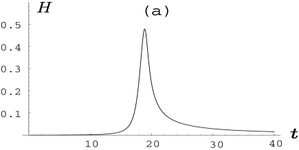
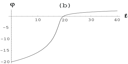
FIG. 1.: The cosmological solution obtained from the action (1). The universe makes a smooth transition from accelerating phase to Friedmann-like phase. After the transition the scalar field loses its kinetic energy and slows down.

Cosmologically interesting solution which leads to a Friedmann-like universe in late time is such that $H>0$. This solution describes the universe which starts from a Minkowski space with large enough $|\varphi|$ at $t=-\infty$, gradually accelerates its expansion and increases the moduli kinetic energy as

$$H\sim\frac{\omega_{1}}{|t|^{2}},\hskip 2.84526pt\varphi\sim\varphi_{p}-5\ln|t|,\hskip 2.84526pt\dot{\varphi}\sim\frac{5}{|t|},\hskip 2.84526pta\sim a_{p},$$ (6)

where $\omega_{1}$, $a_{p}$, and $\varphi_{p}$ are constants. The constraint equation (3) gives a relation $5e^{\varphi_{p}}=2\omega_{1}^{3}\pi$ between the initial values, so the initial degree of the freedom is only one, apart from the overall scaling of $a_{p}$. Note that, reflecting the special choice of the higher derivative terms (the Gauss-Bonnet combination), there are no redundant degrees of freedom which may make the phase space unphysically large. Subsequently, the Hubble parameter reaches its maximal value $H=H_{\max}$ at $\varphi\sim 0$, where moduli loses its kinetic energy and slows down. After the Hubble peak, the universe naturally goes into a Friedmann-like phase, where

$$H\sim\frac{1}{3t},\hskip 2.84526pt\varphi\sim\sqrt{\frac{2}{3}}\ln t,\hskip 2.84526pta\sim a_{f}t^{\frac{1}{3}}.$$ (7)

Here, $a_{f}$ is a constant. An example of the numerical solution is shown in Fig. 1. In this model, there is no horizon problem since there is no particle horizon. It is worth mentioning that this model is not plagued by a running scalar field, since the scalar field slows down in the Friedmann-like phase, which is similar to the Damour-Polyakov mechanism[6].

III Cosmological evolution

Realistic cosmological models need to explain the thermal equilibrium in the early universe and the generation of present cosmological structures. Following the usual inflationary scenario, we assume that the reheating is caused by the coherent oscillation of the inflaton at the end of the chaotic inflation which started shortly after the Hubble peak in the model described in the preceding section. This chaotic inflation is caused by the large fluctuation around the Hubble peak which kicks up the inflaton to sufficiently large expectation value.

As a component of the matter Lagrangian, we assume the inflaton Lagrangian of the form,

$${\cal L}_{inflaton}=-\frac{1}{2}(\nabla\chi)^{2}-V(\chi),$$ (8)

where for simplicity we only consider the potential

$$V(\chi)=\frac{1}{4}g\chi^{4}.$$ (9)

After the Hubble parameter reaches its peak, the inflaton expectation value becomes large due to the large fluctuation. The universe region with sufficiently large $\chi$ satisfies the slow-roll condition and inflates. A natural initial condition for the chaotic inflation is estimated as

$$M_{P}^{2}H_{I}^{2}\simeq\frac{1}{4}g\chi_{I}^{4}.$$ (10)

The subscript $I$ denotes the value at the beginning of the chaotic inflation, which is supposed to be shortly after the Hubble peak. Then the e-folding number of the chaotic inflation is determined by the initial value of the inflaton as

$$N\simeq\frac{\pi\chi_{I}^{2}}{M_{P}^{2}}.$$ (11)

In our scenario there are four distinct eras. The first is the superinflationary era, which we call SI for short, with increasing Hubble parameter and accelerating modulus field. The second is the chaotic inflationary era, denoted CI, where the Hubble parameter stays constant and the scale factor increases exponentially. At the end of this chaotic inflation the energy of the oscillating inflaton is converted into radiation, and the universe becomes radiation dominated (RD). As the radiation is redshifted away more quickly than the matter, in the course of time the universe will be matter dominated (MD).

IV Perturbation spectra

In our scenario, the inhomogeneity of the universe, which is expressed as the perturbation on the homogeneous universe, is generated as the quantum fluctuation inside the horizon. The quantum fluctuation is once red-shifted out of the horizon and classicalized in SI and CI eras, and reenters inside the horizon in RD and MD eras. Since this inhomogeneity is supposed to be the seeds of the large scale structure of the present universe, the spectrum of the fluctuation is crucial in predicting the large scale structure today and thus in discussing the plausibility of this scenario. In this section, we speculate on the quantum fluctuation spectra generated during the SI and CI eras.

A Adiabatic perturbation from superinflation

In order to describe the fluctuations we expand the metric and the modulus up to first order of perturbations:

$$ds^{2} = -(1+2\phi)dt^{2}+2aV_{|i}dtdx^{i}$$ (13)

$$+a^{2}\left\{(1-2\psi)\delta_{ij}+2E_{|ij}\right\}dx^{i}dx^{j},$$

$$\varphi = \varphi^{(0)}+\delta\varphi.$$ (14)

For the study of the fluctuations in SI era, it is convenient to use the uniform field gauge ($\delta\varphi=0$, $E=0$). In this gauge the perturbation of the Einstein equation reduces to one wave equation[7]

$$\ddot{\psi}+\frac{\dot{A}}{A}\dot{\psi}+B\frac{\nabla^{2}}{a^{2}}\psi=0,$$ (15)

where

$$A=\frac{a^{3}\alpha(5\alpha^{2}-2\alpha+1)}{(3\alpha-1)^{2}},$$ (16)

$$B=\frac{(\alpha-1)^{2}(3\Gamma-2)}{5\alpha^{2}-2\alpha+1}-1.$$ (17)

Here, $\alpha$ and $\Gamma$ are defined as $\alpha=1-H\dot{\xi}$ and $\Gamma=-2\dot{H}/3H^{2}$, respectively. As can be seen from (3), $\alpha$ is (proportional to) the fraction of the modulus kinetic energy to the geometrical kinetic energy. $\Gamma$ is the effective adiabatic index $\Gamma-1=-G^{i}{}_{i}/3G^{0}{}_{0}$, where $G^{\mu}{}_{\nu}$ is the background Einstein tensor. They behave as $\alpha\sim t^{2}$, $\Gamma\sim t$ in the past asymptotic region and $\alpha\sim 1$, $\Gamma\sim 2$ in the future asymptotic region (in the sense of (7)). Since the scale factor is almost constant in the past region, $a^{3}\alpha$ rapidly decreases as the universe evolves towards the Hubble peak. This leads to a decrease of the effective volume $A$ and the perturbation behaves as if the universe is collapsing. Note that the other variables $\phi$ and $V$ are written in term of $\psi$, as

$$\phi=\frac{2\alpha\dot{\psi}}{(1-3\alpha)H},$$ (18)

$$V=\frac{1}{a^{2}\alpha}\int a\alpha\left[(3\Gamma-5)\psi-\phi\right]dt.$$ (19)

In the ordinary inflationary universe scenario, the fluctuation is quantum mechanically generated inside the horizon and is classicalized as it is stretched to superhorizon. We assume the similar picture in SI era as well as in CI era. According to the conventional prescription, we regard $\psi$ as an Schrödinger operator and decompose it into mode functions

$$\hat{\psi}=\int d^{3}k(2\pi)^{-3/2}\left\{\hat{a}_{k}u_{k}(t)e^{ikx}+\hat{a}_{k}^{\dagger}u_{k}^{*}(t)e^{-ikx}\right\},$$ (20)

where $\hat{a}_{k}$ and $\hat{a}_{k}^{\dagger}$ are annihilation and creation operators satisfying the commutation relation $\left[\hat{a}_{k},\hat{a}_{q}^{\dagger}\right]=\delta^{3}(k-q).$ The mode functions $u_{k}$ and $u_{k}^{*}$ are determined so that $\hat{\psi}$ satisfies the equation (15). Using the past asymptotic solutions (6) in the superinflationary regime, the equation for $u_{k}$ becomes

$$\ddot{u}_{k}+\frac{2}{t}\dot{u}_{k}-\frac{4tk^{2}}{5\omega_{1}a_{p}^{2}}u_{k}=0.$$ (21)

The canonically normalized solution of this equation which reduces to a positive frequency mode in the short wavelength limit ($k\gg aH$) will be

$$u_{k}=\frac{N_{k}}{t}\left[\mbox{Bi}\left(\left(\frac{4k^{2}}{5\omega_{1}a_{p}^{2}}\right)^{1/3}t\right)+i\mbox{Ai}\left(\left(\frac{4k^{2}}{5\omega_{1}a_{p}^{2}}\right)^{1/3}t\right)\right],$$ (22)

where Ai and Bi are the Airy functions and $N_{k}$ is the normalization factor

$$N_{k}=\pi^{1/2}\left(\frac{k}{a_{p}}\right)^{-1/3}\left(\frac{3}{5a_{p}}\right)^{3/2}\left(\frac{5\omega_{1}^{7}}{4}\right)^{1/6}.$$ (23)

The long wavelength limit ($k\ll aH$) of this positive mode function represents the behavior of the perturbations outside the horizon. The power spectrum estimated shortly after the Hubble peak has the form

$$P_{\psi}=\frac{k^{3}}{2\pi^{2}}|\psi_{k}|^{2}\sim{\cal O}(10^{-1})\times\omega_{1}^{\frac{5}{3}}\left(\frac{k}{a_{p}}\right)^{\frac{7}{3}}\left(\frac{a_{p}}{a_{*}}\right)^{6},$$ (24)

where the asterisk denotes the values estimated at (or more precisely, just after) the Hubble peak. This is a steep blue spectrum with a spectral index $n_{\psi}=d\ln P_{\psi}/d\ln k+1=10/3$. It should be noted that this expression includes no independent variables, and is determined only by one background initial condition $\omega_{1}$. Thus the amplitude of the fluctuation is determined unambiguously once the background is fixed.

B Isocurvature perturbation from superinflation

Apart from the adiabatic fluctuation described above, there is another possible source of the fluctuation with significantly different spectrum in SI era. We consider a matter Lagrangian of an axionic field[9],

$${\cal L}_{matter}=-\frac{1}{2}e^{2\mu\varphi}(\nabla\sigma)^{2}.$$ (25)

We decompose the axion field into its background part and a small perturbation, $\sigma=\sigma^{(0)}+\delta\sigma$, and suppose $\sigma^{(0)}=0$ so that the background cosmological solution and the perturbation $\psi$ are unaffected by the introduction of this axionic field. The equation for $\delta\sigma$ is

$$\delta\ddot{\sigma}+(3H+2\mu\dot{\varphi})\delta\dot{\sigma}-\frac{\nabla^{2}}{a^{2}}\delta\sigma=0,$$ (26)

and the canonical quantization of $\delta\sigma$ using the past asymptotic background solution (6) yields the spectrum

$$P_{\delta\sigma}=\frac{1}{8\pi^{3}}\left(\frac{5}{2\omega_{1}^{3}\pi}\right)^{2\mu}\left(\frac{k}{a_{p}}\right)^{2-10\mu}2^{10\mu+1}\Gamma(5\mu+\frac{1}{2})^{2}.$$ (27)

The spectral index, $n_{\delta\sigma}=d\ln P_{\delta\sigma}/d\ln k+1=3-10\mu,$ depends on the coupling $\mu$. For $\mu=0.2$, this gives a scale invariant flat spectrum. It is noted that the statistics of this fluctuation is non-Gaussian.

C Perturbation from chaotic inflation

Finally, there is a perturbation of flat $n=1$ spectrum arising from the chaotic inflation. The amplitude of the density fluctuation at the horizon is estimated as

$$\zeta_{\lambda}\sim\left(\frac{H^{2}}{\dot{\phi}}\right)_{\lambda}\simeq 2\sqrt{\frac{2}{3}}g^{1/2}N_{\lambda}^{3/2}.$$ (28)

Here, $N_{\lambda}$ is the e-folding number of the chaotic inflation since the scale $\lambda$ under consideration exits the horizon, until the time of reheating. Similarly, $\zeta_{\lambda}$ is the value for the corresponding comoving fluctuation scale $\lambda$.

D Fluctuation spectrum in our scenario

To sum up what have been calculated, we have three sources of perturbations with different spectra:
1) Adiabatic perturbation of $n_{\psi}=10/3$ blue spectrum from superinflationary era,
2) Isocurvature perturbation of $n_{\delta\sigma}=3-10\mu$ spectrum from superinflationary era,
3) Adiabatic perturbation of $n_{\chi}=1$ flat spectrum from chaotic inflationary era.

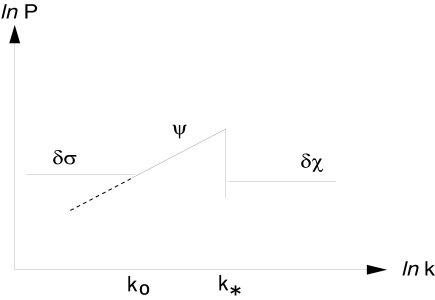
FIG. 2.: Perturbation spectra in our scenario. $\delta\sigma$ is the isocurvature perturbation and $\psi$ is the adiabatic perturbation generated in the superinflationary era. In this figure the perturbation $\delta\sigma$ is drawn as flat, but this can be tilted to red or blue, depending on the axion type coupling constant $\mu$ which is chosen accordingly. The wavenumber corresponding to the horizon scale at the Hubble peak is denoted by $k_{*}$. The other indicated wavenumber $k_{o}$ corresponds to the scale where the amplitude of $\psi$ becomes comparable to that of $\delta\sigma$.

There might exist other sources of perturbations, such as the isocurvature mode perturbation during CI era. However, we neglect them and assume these three perturbations dominate for different scales and determine the whole primordial density perturbations. Since the universe is always expanding, the perturbation generated in earlier time is expanded to larger scale at present. Fig. 2 shows the expected perturbation spectra in our model, where $\delta\sigma$ and $\psi$ is the isocurvature and adiabatic perturbations, respectively, in SI era and $\delta\chi$ is the adiabatic perturbation in CI era. The inclination of $\delta\sigma$ can be tilted in either blue or red direction depending on $\mu$. The figure shows the flat case where $\mu=0.2$.

V Structure formation history

Let us discuss the observational viability of our scenario. In this model there are two distinct scales in fluctuations. One is the scale corresponding to the horizon scale of the Hubble peak, which we denote by $\lambda_{*}$. The comoving wave number corresponding to this scale, $k_{*}=2\pi a/\lambda_{*}$, is shown in Fig. 2. The other scale, $\lambda_{o}$, is where the amplitude of the blue adiabatic perturbation ($\psi$) is comparable to that of the isocurvature perturbation ($\delta\sigma$). The corresponding comoving wave number $k_{o}=2\pi a/\lambda_{o}$ is also shown in Fig. 2. These scales are determined by the reheating temperature $T_{rh}$ and the initial inflaton value $\chi_{I}$, through the e-folding number during and after the chaotic inflation up to present. Here we discuss two examples with explicit parameter values.

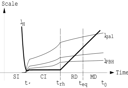
FIG. 3.: A schematic picture of the Hubble horizon scale $\ell_{H}$ and the perturbation scales in our scenario. Shortly after the Hubble peak the inflaton acquires a large expectation value owing to the large fluctuations, and the chaotic inflation starts. At the end of the chaotic inflation the universe is heated by the coherent oscillation of the inflaton. See Sec. VB for the explanations of the scales $\ell_{gal}$ and $\ell_{PBH}$.

A CI structure formation scenario

We first consider the case where the scale $\lambda_{*}$ is large enough compared to the horizon scale today, so that all of the observable structures are generated during the CI era. In this case our scenario is nothing but that of the ordinary chaotic inflation, though the history before the onset of the chaotic inflation is included in our picture. Since the evidence of the singularity avoidance (the physics around the Hubble peak) has been inflated away beyond the present horizon, this model is consistent with our current observations only if the chaotic inflation successfully takes place and generates appropriate amount of fluctuations. In order to predict the fluctuation amplitude of ${\cal O}(10^{-5})$, the coupling constant has to be $g\simeq{\cal O}(10^{-15})$. If we assume the constant Hubble parameter during the CI to be $10^{-7}M_{P}$, then the condition (10) implies $\chi_{I}\simeq 4.9M_{P}$. From (11), the e-folding number of the CI era will be $N\simeq 74$ and we can see that the present horizon scale ($\sim\mbox{Gpc}$) is generated within the CI era. Thus, with appropriate choice of parameters, the chaotic inflation naturally takes place and generates fluctuations with observationally acceptable amplitude.

B SI structure formation scenario

As another possible scenario of structure formation, we can consider the case where both $\lambda_{o}$ and $\lambda_{*}$ are inside the horizon today. In this case, what generates the observationally supported nearly flat spectrum which evolves to the present large scale structure, is the isocurvature perturbation[10] of SI era with appropriate choice of $\mu$ . Then the outstanding pointed spectrum of the $\psi$ perturbation and the flat spectrum of $\delta\chi$ perturbation, as is shown in Fig. 3, come inside the present horizon. This may fall into the scale of observational interest. We choose, for example, the parameters as

$$H_{*}=0.1M_{P},\hskip 5.0pt\mu=0.12,\hskip 5.0ptg=10^{-12},\hskip 5.0pt\chi_{I}=4.6M_{P},$$ (29)

$$\hskip 5.0ptT_{rh}=10^{12}~{}\mbox{GeV},\mbox{~{}and~{}}H_{CI}=H_{I}=10^{-5}M_{P}.$$ (30)

Here, $H_{CI}$ is the energy scale of the chaotic inflation, which follows from the condition (10). Using (11), the e-folding number of the chaotic inflation is estimated as $N\sim 67$. Taking account of the reheating temperature of $10^{12}$ GeV and rather high energy scale $10^{-5}M_{P}$ during CI era, the large scale fluctuation of the universe which we observe today as CMB corresponds to the scale which exits the horizon during SI era. From $\mu=0.12$, the isocurvature perturbation during the superinflationary era has a blue tilted spectrum with $n_{\delta\sigma}=1.8$. The amplitude of the fluctuation for the present horizon scale is, from (27) with $\omega_{1}\simeq 0.1$ and $a_{*}/a_{p}\simeq 5$, estimated as $P_{\delta\sigma}^{1/2}\sim 10^{-3}$.

The fluctuation generated during the chaotic inflation comes to scales smaller than kpc today. If the amplitude of this small scale perturbation is too large, it will produce primordial blackholes. The primordial blackholes of masses smaller than $10^{15}$ g will Hawking-evaporate within the age of the universe, and if the radiation emitted through the evaporation is too strong, it will spoil the observationally supported nucleosynthesis scenario. Thus the amplitude of this small scale perturbation is constrained by the amount of the primordial blackholes. Assuming the spherical collapse model with Gaussian perturbation, the primordial blackhole mass fraction at the time of their formation is estimated in terms of the perturbation amplitude $\delta(M)$ for the mass scale $M$ as[11],

$$\beta(M)\simeq\delta(M)\exp\left(-\frac{1}{18\delta^{2}(M)}\right).$$ (31)

The strongest constraint for the amount of the small blackholes is $\beta/(1-\beta){}^{\displaystyle<}_{\displaystyle\sim}10^{-26}$[12]. Using our choice of the parameters (30), the amplitude of the perturbation generated during CI era, from (28), is $\delta\sim 10^{-4}$. Substituting this into (31), we can see that the small primordial blackholes are not overproduced.

The adiabatic perturbation of $n_{\psi}=10/3$, whose maximal amplitude is determined by (24), will produce certain amount of primordial blackholes on its horizon reenter. The mass of these blackholes is determined, according to the standard scenario of primordial blackhole formation, by the Hubble horizon scale at the time of reenter. In our scenario the sharp peak of the fluctuation spectrum exits the horizon at $t_{*}$, inflated by the chaotic inflation and reenters the horizon during the radiation dominated era of the universe. For our parameters (30), the scale of the perturbation peak enters the horizon where $H\sim 10^{-2}\mbox{sec}{}^{-1}$. Then the mass of the typical primordial blackholes generated by the $n_{\psi}=10/3$ spectrum is $M\sim 10^{7}M_{\odot}$. The amount of these blackholes can be estimated by using (31). We have $\delta\simeq P_{\psi}^{1/2}\simeq 0.05$ for our parameters, so $\beta\simeq 10^{-10}$ at the time of horizon reenter. Translating this into the present fraction of the blackholes with respect to the whole energy density of the universe, we have $\Omega_{BH}\sim 10^{-6}$. Since the spectrum of the adiabatic perturbation in SI era is steeply blue, its contribution to the perturbation amplitude in larger scales is negligible.

Recent observations suggest the existence of supermassive blackholes of masses $10^{7}\sim 10^{9}M_{\odot}$ at the galactic center. The amount of these blackhole is estimated using the radiation from the quasar, which is emitted along with the accretion of matter onto the blackholes[13]. The mass density of dead quasars is estimated as $\rho_{\bullet}=u/\epsilon c^{2}\simeq 2.2\times 10^{5}(0.1/\epsilon)M_{\odot}/\mbox{Mpc}^{3}$, which follows from the observed radiation density of quasars, $u\sim 1.3\times 10^{-15}\mbox{erg}/\mbox{cm}^{3}$. In the expression of $\rho_{\bullet}$, $\epsilon$ is the efficiency of the radiation process. Assuming that the mass density of dead quasars are comparable to that of blackholes, this indicates $\Omega_{BH}\sim 10^{-6}$. Thus, our model with parameter values (30) predicts both mass and density of the blackholes which are typically found in galactic centers.

VI Discussions

We have described a structure formation scenario based on a higher curvature non-singular cosmological model, and discussed two examples with explicit parameter values. Our rough estimates show that, with appropriate choice of parameters, this model can produce observationally acceptable amount of perturbation amplitude in large scales, and even primordial blackholes in interesting mass scales.

We have just assumed that the chaotic inflation, due to the large fluctuation, takes place after the Hubble peak, and we have not discussed the physics of the onset of the chaotic inflation in detail. Of course there is a room to discuss other possibilities by including other fields, etc., but this is beyond the scope of this paper. Here, we comment on one possible alternative scenario based on the study of the perturbation behavior. Our background cosmological solution depends on the initial condition with only one degree of freedom. In stead of $\omega_{1}$ in the discussion above, here we specify the background by $H_{*}$, the maximum Hubble parameter. For universes with small $H_{*}$, $B$ of (17) remains negative throughout the evolution of the universe. For $H_{*}$ larger than unity in our unit, there appears shortly after the Hubble peak a period where $B$ becomes positive so the perturbation becomes unstable in short length[8]. Since our unit is roughly Planckian, the Hubble parameter of the threshold of the instability is Planck scale. If this instability is physical, the perturbation inside the horizon will grow exponentially in time and the region inside the horizon will collapse to form Planckian scale primordial black holes. Since small scale blackholes evaporate almost instantly, the universe will be heated by the Hawking evaporation of these Planckian scale blackholes. Assuming that most of the energy density is converted to radiation during the unstable period, the reheating temperature of this scenario would be estimated as $H^{2}\sim\frac{1}{2}\dot{\varphi}^{2}\sim N_{eff}T_{rh}^{4}$, indicating the reheating temperature around the Planckian temperature. Here, $N_{eff}$ is the number of particle species at the reheating epoch. If this reheating takes place, we have to consider a thermal inflation rather than the chaotic inflation in the following scenario. This inflation is necessary in order to dilute unwanted relics coming out of the evaporating blackholes. This scenario, however, might be somewhat speculative, and considering that the action of our starting point (1) is obtained by the loop correction in the string theory, a sensible interpretation would be that the effective theory breaks down for $H{}^{\displaystyle>}_{\displaystyle\sim}{\cal O}(1)$ and that this instability is unphysical.

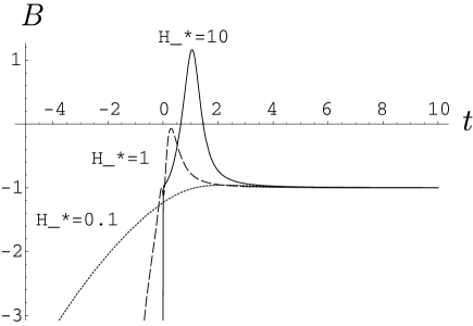
FIG. 4.: The time evolution of B (17) for different background solutions which are specified by different values of $H_{*}$. Note that these are calculated on the numerical solutions of (3-5), and no further assumptions such as the continuation to the CI era are taken into account. As can be seen from (15), positive B means the existence of the instability for the scales smaller than the Hubble horizon.

A Formulae of cosmological perturbations

The equations of motion derived from the effective action (1) can be written as the following Einstein equation:

$$G^{\mu}{}_{\nu}=T_{\varphi}{}^{\mu}{}_{\nu}+T_{GB}{}^{\mu}{}_{\nu}+T_{matter}{}^{\mu}{}_{\nu},$$ (A1)

where

$$G^{\mu}{}_{\nu} = R^{\mu}{}_{\nu}-\frac{1}{2}R\delta^{\mu}{}_{\nu},$$ (A2)

$$T_{\varphi}{}^{\mu}{}_{\nu} = \varphi^{;\mu}\varphi_{;\nu}-\frac{1}{2}\varphi^{;\alpha}\varphi_{;\alpha}\delta^{\mu}{}_{\nu},$$ (A3)

$$T_{GB}{}^{\mu}{}_{\nu} = (R^{\mu}{}_{\alpha\nu\beta}-R_{\alpha\beta}\delta^{\mu}{}_{\nu}+R_{\alpha\nu}\delta^{\mu}{}_{\beta})\xi^{;\alpha\beta}$$ (A5)

$$+G^{\mu}{}_{\alpha}\xi^{;\alpha}{}_{;\nu}-G^{\mu}{}_{\nu}\xi^{;\alpha}{}_{;\alpha},$$

$$T^{matter}_{\mu\nu} = \frac{1}{2\sqrt{-g}}\frac{\delta{\cal L}_{matter}}{\delta g^{\mu\nu}}.$$ (A6)

The non-vanishing components of $T_{GB}{}^{\mu}{}_{\nu}$ are

$$T_{GB}{}^{0}{}_{0} = {}-3H^{3}\dot{\xi},$$ (A7)

$$T_{GB}{}^{i}{}_{j} = {}-\left[H^{2}\ddot{\xi}+2(\dot{H}+H^{2})H\dot{\xi}\right]\delta^{i}{}_{j}.$$ (A8)

Expanding $T_{GB}{}^{\mu}{}_{\nu}$ up to first order in perturbation gives

$$\delta T_{GB}{}^{0}{}_{0} = \frac{\nabla^{2}}{a^{2}}\left[H^{2}\delta\xi+3aH^{2}\dot{\xi}(V-a\dot{E})-2H\dot{\xi}\psi\right]$$ (A10)

$$+12H^{3}\dot{\xi}\phi+9H^{2}\dot{\xi}\dot{\psi}-3H^{3}\dot{\delta\xi},$$

$$\delta T_{GB}{}^{0}{}_{i} = \frac{\nabla_{i}}{a}\left[H^{2}\dot{\delta\xi}-H^{3}\delta\xi-3H^{2}\dot{\xi}\phi-2H\dot{\xi}\dot{\psi}\right],$$ (A11)

$$\delta T_{GB}{}^{i}{}_{j} = \frac{\nabla^{i}\nabla_{j}-\delta^{i}_{j}\nabla^{2}}{a^{2}}\left[\ddot{\xi}\psi-H\dot{\xi}\phi-\frac{1}{a}\left\{a^{2}H\dot{\xi}(V-a\dot{E})\right\}\dot{}\right.$$ (A15)

$$-\left.(\dot{H}+H^{2})\delta\xi\right]+\left[2H\ddot{\psi}+2(\dot{H}+3H^{2}+H\ddot{\xi})\dot{\psi}\right.$$

$$+\left.3H^{2}\dot{\phi}+4H\left\{2\dot{\xi}(\dot{H}+H^{2})+H\ddot{\xi}\right\}\phi-H^{2}\ddot{\delta\xi}\right.$$

$$-\left.2(H^{3}+H\dot{H})\dot{\delta\xi}\right]\delta^{i}{}_{j}.$$

In the uniform field gauge, the equations of motion for the perturbations (neglecting $T_{matter}^{\mu\nu}$) become:

$$3(3\alpha-1)H\dot{\psi}-6H^{3}\dot{\xi}\phi=2\alpha\frac{\nabla^{2}}{a^{2}}\psi-(3\alpha-1)H\frac{\nabla^{2}}{a^{2}}V,$$ (A16)

$$(3\alpha-1)H\phi+2\alpha\dot{\psi}=0,$$ (A17)

$$\alpha\phi-(3\Gamma-5)\alpha\psi+\frac{1}{a}(a^{2}\alpha V)\dot{}=0,$$ (A18)

$$\ddot{\psi}+3H\dot{\psi}+H(1-\frac{3}{2}H\dot{\xi})\dot{\phi}$$ (A19)

$$\mbox{\hskip 56.9055pt}=(H\dot{\xi}\dot{\psi})\dot{}+(H\ddot{\xi}+2H^{2}\dot{\xi}+2\dot{H}\dot{\xi})H\phi.$$ (A20)

These four equations reduce to the wave equation (15).

REFERENCES

- [1] A. Vilenkin, Phys. Rev. D 46, 2355 (1992).
- [2] A. Vilenkin, Phys. Lett. 117B 25 (1982), Phys. Rev. D 27 2848 (1983); J. B. Hartle and S. W. Hawking, Phys. Rev. D 28, 2960 (1983).
- [3] V. F. Mukhanov, and R. H. Brandenberger, Phys. Rev. Lett. 68, 1969 (1992); R. Brandenberger, V. Mukhanov, and A. Sornborger, Phys. Rev. D 48, 1629 (1993).
- [4] I. Antoniadis, E. Gava and K. S. Narain, Nucl. Phys. B 383, 93 (1992);
- [5] I. Antoniadis, J. Rizos and K. Tamvakis, Nucl. Phys. B 415, 497 (1994); J. Rizos and K. Tamvakis, Phys. Lett. B 326, 57 (1994); R. Easther and K. Maeda, Phys. Rev. D 54, 7252 (1996); P. Kanti, J. Rizos, K. Tamvakis, Phys.Rev. D 59, 083512 (1999). D.
- [6] T. Damour and A. M. Polyakov, Nucl. Phys. B 423, 532 (1994), Gen. Relativ. Grav.t. 26, 1171 (1994); T. Damour and A. Vilenkin, Phys. Rev. D 53, 2981 (1996).
- [7] J. Hwang and H. Noh, “Conserved cosmological structures in the one-loop superstring effective action”, to be published.
- [8] S. Kawai and J. Soda, Phys.Lett. B 460 41 (1999).
- [9] E. J. Copeland, J. E. Lidsey and D. Wands, Nucl.Phys. B 506, 407 (1997), Phys. Lett. B 443, 97 (1998); E. J. Copeland, R. Easther, and D. Wands, Phys. Rev. D 56, 874 (1997).
- [10] G. Efstathiou and J. R. Bond, Mon. Not. R. Astron. Soc. 218, 103 (1986).
- [11] B. J. Carr, Astrophys. J. 201, 1 (1975). (1994).
- [12] I. D. Novikov, A. G. Polnarev, A. A. Starobinski, Ya. B. Zel’dovich, Astron. Astrophys. 80, 104 (1979); B. J. Carr and J. E. Lidsey, Phys. Rev. D 48, 543 (1993); B. J. Carr, J. H. Gilbert and J. E. Lidsey, Phys. Rev. D 50, 4853 (1994); J. Yokoyama, Phys. Rev. D 58 107502 (1998).
- [13] Chokshi and Turner, MNRAS 259 421 (1992); Soltan, MNRAS 200 115 (1982).