Energy Absorption by the Dilaton Field around a Rotating Black Hole in a Binary System

Abstract

In this paper we analyze a binary system consisting of a star and a rotating black hole. The electromagnetic radiation emitted by the star interacts with the background of the black hole and stimulates the production of dilaton waves. We then estimate the energy transferred from the electromagnetic radiation of the star to the dilaton field as a function of the frequency. The resulting picture is a testable signature of the existence of dilaton fields as predicted by string theory in an astrophysical context.

I Introduction

The theory of strings and membranes is a very attractive candidate for the quantum theory of gravity, however, few results have been derived which can be tested at present. In this approach, our Universe is supposed to be described by the low energy effective action of string theory. The latter can be written in terms of the fields associated with the massless excitations of extended objects, among which there is a scalar field (the dilaton) (see, e.g., Ref. [1]). In a series of papers [2, 3, 4, 5, 6, 7, 8, 9] we have explored the viewpoint that quantum black holes are massive excitations of extended objects and hence are elementary particles. Our goal is thus to obtain expressions which can be compared to experimentally measurable quantities in order to test the idea that quantum black holes are extended objects. In all likelihood the scalar component of gravity, provided it does not acquire a mass from quantum corrections [1], will have a coupling to electromagnetic waves which is as weak as that of the tensor component. Therefore the best place to look for the effect of the long range dilaton on electromagnetic waves is in the neighborhood of a black hole, which we consider to be composed of quantum black holes.

In Ref.[10], starting from the low energy effective action describing the Einstein-Maxwell theory interacting with a dilaton $\phi$ in four dimensions $(G=1)$ [11],

$$S={1\over 16\,\pi}\,\int d^{4}x\,\sqrt{-g}\,\left[R-{1\over 2}\,(\nabla\phi)^{2}-e^{-a\,\phi}\,F^{2}\right]\ ,$$ (1)

we obtained the static solutions of the field equations for a Kerr-Newman dilaton (KND) black hole rotating with arbitrary angular momentum by expanding the fields in terms of the charge-to-mass ratio of the black hole. In [12, 13] we used these solutions, which appear as a background in the linear wave equations, to investigate the effects of the background dilaton on the propagation of various spin waves in the vicinity of a rotating charged black hole. In particular, we showed that the different wave modes disentangle at a given order in the charge-to-mass expansion and this allowed us to study the electromagnetic waves analytically up to second order in the charge-to-mass ratio.

The point of view we take in the present paper is more phenomenological in that we focus on the search for observable effects. We want to model a binary system which is composed of a rotating black hole and a star and estimate the perturbation that would be induced on the electromagnetic spectrum of the star, as detected by a distant observer, by the existence of a scalar component of gravity. This does not require the presence of a static dilaton field, nor does the black hole itself need to be electrically charged. All that is needed is a background electromagnetic field whose source could be, e.g., in the accreting disk which we consider as part of the black hole component of the binary system.

In particular, we shall be interested in the case when the plane containing the system is roughly parallel to the direction of observation since then we expect stronger contributions. This configuration implies that when the star is in front of the black hole, the background of the black hole negligibly affects the radiation coming from the star. On the other hand, when the star is going behind the black hole, the radiation emitted by the star will travel across a region where the static electromagnetic field is stronger. The leading order effect is then the interaction between electromagnetic waves and the electromagnetic background which produces dilaton waves, thus carrying away a certain amount of energy. This energy can be transferred from dilaton modes back in the form of electromagnetic radiation or to gravitational waves, both cases being next order in the dilaton coupling constant and in the charge-to-mass ratio in our approximation scheme [12, 13]. Therefore we shall assume that the dilaton waves retain most of their energy and simply result in a permanent loss from observation. We shall then study the dilaton wave equation and estimate the energy lost by the radiation of the star so that, by comparing the spectra corresponding to the two different relative positions of the star and the black hole, one can infer (or disprove) the existence of scalar gravitational excitations.

We begin in Section II with a detailed description of the system under study, the governing equations and the approximations we will assume in order to manage the equations analytically. In Section III we obtain expressions for the dilaton waves generated by the radiation emitted by the star. Finally, in Section IV we estimate the energy flux at large distance and in Section V discuss our results. For the notation and the complete description of the background of the rotating black hole we refer to [10]; for the derivation of linear perturbations the main reference is [12].

II The binary system

We consider a binary system made of a star and a rotating black hole. If the black hole is electrically charged, then from string theory one expects a non-trivial background dilaton field [10]. However, as we mentioned in the Introduction, the charge does not need to be located in the black hole singularity itself. In fact, the metric we shall be using to describe the black hole (as well as any other black hole metric) works well for the exterior of any rotating charged distribution of matter. Given any charge distribution in the matter just outside the horizon, one could then approximate the true metric everywhere by pasting together regions where the metric is given by Eq. (2) below with different values for its parameters. For the sake of simplicity, in the following we shall consider only one set of parameters for all points in the region of interest.

We shall also assume that the presence of the star does not affect the geometry of space-time significantly in the region near the outer horizon of the black hole (denoted by $r_{+}$) where the static electromagnetic field is presumably stronger. This means that either the mass of the star is much smaller than the black hole ADM mass $M$ or that the star is distant enough from the black hole. In both cases we approximate the background metric in the region of interest by [10]

$$ds^{2}=-\Psi\,(dt-\omega\,d\varphi)^{2}+{\Delta\,\sin^{2}\theta\over\Psi}\,(d\varphi)^{2}+\rho^{2}\,\left[{(dr)^{2}\over\Delta}+(d\theta)^{2}\right]\ ,$$ (2)

in which $x^{0}=t$, $x^{1}=r$, $x^{2}=\theta$, $x^{3}=\varphi$ are Boyer-Lindquist coordinates centered on the black hole. The explicit expressions of the functions $\Psi=\Psi(r,\theta)$, $\omega=\omega(r,\theta)$ and $\Delta=\Delta(r)$ in terms of the mass $M$, charge $Q$ and angular momentum $J=\alpha\,M$ of the hole coincide (at order $Q^{2}/M^{2}$) with the Kerr-Newman (KN) metric [12, 14]

$$\Delta = r^{2}-2\,M\,r+\alpha^{2}+Q^{2}$$ (3)

$$\rho^{2} = r^{2}+\alpha^{2}\,\cos^{2}\theta$$ (4)

$$\Psi = -(\Delta-\alpha^{2}\,\sin^{2}\theta)/\rho^{2}$$ (5)

$$\omega = -\alpha\,\sin^{2}\theta\,[1+\Psi^{-1}]\ .$$ (6)

Another basic observation is that, although the system is approximately axisymmetric, if the star revolves along a circular orbit around the black hole, the pattern of the radiation emitted by the star does not share this symmetry, which renders the analysis extremely involved. In fact, following standard Refs. [14, 15] the perturbations on the background (2) have been studied by performing a decomposition into normal modes with angular and radial parts according to this symmetry [12, 13]. Hence, a flux of radiation emitted by the star, which is approximately spherical with respect to the star, should first be decomposed into normal modes on the black hole background, then propagated in the region near the black hole and finally reconstructed at the observation point (far away from the black hole).

In order to speed up the analysis and estimate the order of magnitude of the leading effects, we then focus on a particular configuration of the binary system (Fig. 1). As mentioned in the Introduction, we are interested in orbits of the star which lie roughly along the line of sight of the observer in order to produce occultations. The simplest case is thus to take the orbit of the star, $r_{s}=r_{s}(t)$, in the equatorial plane $\theta=\pi/2$ and assume that it also contains the point of observation $O$. The star must also be sufficiently away from the stationary limit, that is $r_{s}>r_{e}\equiv M+\sqrt{M^{2}-Q^{2}-\alpha^{2}\,\cos^{2}\theta}>r_{+}\equiv M+\sqrt{M^{2}-Q^{2}-\alpha^{2}}$ (for $\theta=\pi/2$), so that it does not affect the background geometry appreciably. Further, the region where the interaction among the various fields is relevant is assumed for convenience to be bounded by the radius $R\sim r_{e}$. Indeed, the parameter $R$ is not related to any basic physical process, rather it is introduced for the purpose of taking into account the finite precision of the measuring devices. The use of such a fictitious parameter follows from the fact that, because of the dependence of the background fields on the distance from the hole, the intensity of the waves produced by the interactions among the various fields falls off as a positive power of $1/r$, where $r$ is the position at which the interaction takes place [12, 13]. As such, $R$ will be kept unspecified and can be taken to infinity or determined at the end by comparing the magnitude of the computed effects with the precision of the measuring apparatus. This will be further discussed in section IV.

Regardless of the actual shape of the orbit of the star we shall consider the following two cases:

i) the star is at a point $A$ between the observer $O$ and the black hole;

ii) the star is at $A^{\prime}$, being occultated by the black hole.

In i) the relevant electromagnetic radiation emitted by the star travels along the line $AO$ and will be approximated by outgoing modes $\phi_{i}^{out}(r)$ ($i=1,2,3$) of the Maxwell equations to leading order in the large $r$ expansion (see next section for the notation and definitions). This is a good approximation since the line $AO$ also contains the black hole, so that deviations from axial symmetry are soft, and $r\geq r_{s}$ is large. Also, since $r$ is presumably bigger than $R$ we assume the electromagnetic radiation propagates freely to the observer (on a Kerr background [12, 14, 15]).

In ii) the path $A^{\prime}O$ breaks the axial symmetry. We then approximate $A^{\prime}O$ with a new path $A^{\prime}CC^{\prime}A^{\prime\prime}O$ and, at first, neglect the contribution from the arc $CC^{\prime}$, so that the electromagnetic radiation always travels along radial lines with respect to the black hole and the normal modes studied in [12] can be used (more accurate estimates of the loss occurring along $CC^{\prime}$ can be obtained from the analysis carried on in section III B 2). In particular, along $A^{\prime}C$ we consider free ingoing modes $\phi_{i}^{in}$ and along $C^{\prime}O$ free outgoing modes $\phi_{i}^{out}$ on the Kerr background. Since the portion of the trajectory between $D$ and $D^{\prime}$ lies inside $R$, this is where the electromagnetic radiation generates other kinds of waves, thus dissipating energy.

A fundamental difficulty in dealing with waves in the axisymmetric space-time of a charged black hole is that electromagnetic, dilaton and gravitational linear waves do not decouple. However, as we mentioned in the Introduction, we have shown in Refs. [12, 13] that it is indeed possible to disentangle the various waves by expanding in the ratio $Q/M$. In this way one finds that each linear wave mode of a given kind at a given order satisfies an equation which contains only the background and wave modes determined at lower orders. This allows one to compute recursively every order in the $Q/M$ expansion (at least in principle, since we know the background only up to order $Q^{3}/M^{3}$) and this will be implemented in the following section for the case at hand.

As a final remark, we warn the reader that, since we consider just one light path at a time, the gravitational lensing of the light coming from the star is not accounted for. The latter is an important relativistic effect which is expected to lead to an increase of the luminosity of the occulting star [16]. Therefore, a detailed balance between the loss of energy we shall compute and the gravitational focusing requires the same analysis to be repeated for all possible light paths emanating from the star and ending in $O$ and their contributions to be summed. Of course, this program is very difficult to carry out analytically and we leave it for future developments.

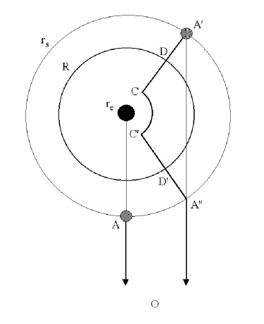
FIG. 1.: The binary system with the light paths as described in the text.

III Linear perturbations of the KND solution

Our input will be given by the electromagnetic waves coming from the star and by examining all wave equations in Ref. [12] one easily realizes that the leading effect in the $Q/M$ expansion is the interaction of ingoing (along $DC$) and outgoing (along $C^{\prime}D^{\prime}$) electromagnetic waves $\phi_{i}^{(1,0)}$ with the (static) electromagnetic background which produces dilatonic waves $\phi_{in/out}^{(1,1)}(r)$. Then, the first step is to compute the solutions of Maxwell’s wave equations at lowest order in $Q/M$ and use these solutions as sources for the dilaton waves. Since we are aiming at computing ratios between the amplitude of the radiation emitted by the star and the amplitude of the dilaton waves generated by the former, we shall not need to take into account the proper normalization of the solutions.

In order to make the present paper self-consistent we now proceed to summarize the notation and review the relevant wave equations for the electromagnetic and dilaton field,

$$\left\{\begin{array}[]{l}\nabla^{i}(e^{-a\,\phi}\,F_{ij})=0\\ \nabla_{[k}F_{ij]}=0\;,\\ \end{array}\right.\ \ {\rm(Maxwell)}$$ (9)

(10)

$$\nabla^{2}\phi=-a\,e^{-a\,\phi}\,F^{2}\ \ \ \ {\rm(dilaton)}\ ,$$ (11)

where $\nabla$ is the covariant derivative with respect to the metric (2).

We will use the standard Newman-Penrose null tetrad vectors [17] for the KN metric [14]

$$l^{i} = {1\over\Delta}\,\left(r^{2}+\alpha^{2},+\Delta,0,\alpha\right)$$ (12)

$$n^{i} = {1\over 2\,\rho^{2}}\,\left(r^{2}+\alpha^{2},-\Delta,0,\alpha\right)$$ (13)

$$m^{i} = {1\over\sqrt{2}\,\bar{\rho}}\,\left(i\,\alpha\,\sin\theta,0,1,i\,\csc\theta\right)\ ,$$ (14)

where $\bar{\rho}\equiv r+i\,\alpha\,\cos\theta$ and $\bar{\rho}^{*}\equiv r-i\,\alpha\,\cos\theta$. Then the spin coefficients are represented by the following Greek letters

$$\kappa=\sigma=\lambda=\nu=\epsilon=0$$ (15)

$$\tilde{\rho}=-{1\over\bar{\rho}^{*}}\ ,\ \ \ \beta={\cot\theta\over 2\,\sqrt{2}\,\bar{\rho}}\ ,\ \ \ \pi={i\,\alpha\,\sin\theta\over\sqrt{2}\,(\bar{\rho}^{*})^{2}}\ ,\ \ \ \tau=-{i\,\alpha\,\sin\theta\over\sqrt{2}\,\rho^{2}}$$ (16)

$$\mu=-{\Delta\over 2\,\rho^{2}\,\bar{\rho}^{*}}\ ,\ \ \ \gamma=\mu+{r-M\over 2\,\rho^{2}}\ ,\ \ \ \tilde{\alpha}=\pi-\beta^{*}\ .$$ (17)

The Maxwell field can be described by three complex quantities,

$$\phi_{0} = F_{ij}\,l^{i}\,m^{j}$$ (18)

$$\phi_{1} = {1\over 2}\,F_{ij}\,(l^{i}\,n^{j}+m^{i}\,m^{*j})$$ (19)

$$\phi_{2} = F_{ij}\,m^{*i}\,n^{j}\ ,$$ (20)

which contain all the information about the six components of the electric and magnetic fields.

We double expand every relevant field in $Q$ and the wave parameter $g$,

$$\phi(t,r,\theta,\varphi)=\sum\limits_{n=0}^{\infty}\,Q^{n}\,\left[\phi^{(0,n)}(r,\theta)+g\,e^{i\,\bar{\omega}\,t+i\,m\,\varphi}\,\phi^{(1,n)}(r,\theta)\right]$$ (21)

$$\phi_{i}(t,r,\theta,\varphi)=\sum\limits_{n=0}^{\infty}\,Q^{n}\,\left[\phi^{(0,n)}_{i}(r,\theta)+g\,e^{i\,\bar{\omega}\,t+i\,m\,\varphi}\,\phi^{(1,n)}_{i}(r,\theta)\right]\ ,\ \ \ i=0,1,2\ .$$ (22)

Each function of $r$ and $\theta$ at order $(1,n)$ implicitly carries an extra integer index, $m$, and the continuous dependence on the frequency $\bar{\omega}$ (both can be positive or negative). The static metric at order zero in the ratio $Q/M$ is given by Eq. (2) with $\Delta$ replaced by $\Delta_{0}=r^{2}-2\,M\,r+\alpha^{2}$. The Maxwell scalars $\phi_{0}^{(0,0)}=\phi_{0}^{(0,1)}=\phi_{2}^{(0,0)}=\phi_{2}^{(0,1)}=\phi_{1}^{(0,0)}=0$ and

$$\phi_{1}^{(0,1)}=-{i\over 2\,(\bar{\rho}^{*})^{2}}\ .$$ (23)

At order $(1,0)$ one obtains the decoupled and separable wave equations in the Kerr background.

In order to write down explicitly Eqs. (11) one needs the directional derivatives along the four null vectors (14) when acting on the wave modes displayed above. Those can be written

$$l^{i}\,\partial_{i} = {\cal D}_{0}$$ (24)

$$n^{i}\,\partial_{i} = -{\Delta\over 2\,\rho^{2}}\,{\cal D}_{0}^{\dagger}$$ (25)

$$m^{i}\,\partial_{i} = {1\over\sqrt{2}\,\bar{\rho}}\,{\cal L}_{0}^{\dagger}$$ (26)

$${m^{*}}^{i}\,\partial_{i} = {1\over\sqrt{2}\,\bar{\rho}^{*}}\,{\cal L}_{0}\ ,$$ (27)

where

$${\cal D}_{n} = \partial_{r}+i\,{K\over\Delta}+2\,n\,{r-M\over\Delta}$$ (28)

$${\cal D}_{n}^{\dagger} = \partial_{r}-i\,{K\over\Delta}+2\,n\,{r-M\over\Delta}$$ (29)

$${\cal L}_{n} = \partial_{\theta}+\tilde{Q}+n\,\cot\theta$$ (30)

$${\cal L}_{n}^{\dagger} = \partial_{\theta}-\tilde{Q}+n\,\cot\theta\ ,$$ (31)

with $n$ an integer such that $n\geq 0$ and $K\equiv(r^{2}+\alpha^{2})\,\bar{\omega}+\alpha\,m$, $\tilde{Q}\equiv\alpha\,\bar{\omega}\,\sin\theta+m\,\csc\theta$.

A Dilaton equation

The equation for the dilaton field at order $(1,0)$ is the Klein-Gordon equation which describes free dilaton waves on the Kerr background. What we need is instead the wave equation at order $(1,1)$,

$$\left[\Delta_{0}\,{\cal D}_{1}\,{\cal D}_{0}^{\dagger}+{\cal L}_{0}^{\dagger}\,{\cal L}_{1}+2\,i\,\bar{\omega}\,\bar{\rho}\right]\Phi=-2\,\sqrt{2}\,a\,\left(\bar{\rho}\,\phi_{1}^{(0,1)}\,\Phi_{1}-\bar{\rho}^{*}\,\phi_{1}^{(0,1)\,*}\,\Phi_{1}^{*}\right)\ ,$$ (32)

where $\phi_{1}^{(0,1)}$ has been given in Eq. (23), $\Phi\equiv\phi^{(1,1)}$ and $\Phi_{1}\equiv\sqrt{2}\,\bar{\rho}^{*}\,\phi_{1}^{(1,0)}$ appearing in the current on the RHS is one of the free Maxwell scalar waves in the Kerr background and represents the flux of radiation emitted by the star. It is important to notice that, due to the form of the current, ingoing (outgoing) Maxwell waves would generate both ingoing and outgoing dilaton waves in the same process.

In the following subsections we compute $\Phi_{1}$ and the corresponding $\Phi$ which we shall use in section IV to estimate the energy absorbed by dilaton waves from the radiation of the star.

B Maxwell waves

As we have just shown we only need the Maxwell waves at order $(1,0)$, thus it is convenient to introduce $\Phi_{0}\equiv\phi_{0}^{(1,0)}$ and $\Phi_{2}\equiv 2\,(\bar{\rho}^{*})^{2}\,\phi_{2}^{(1,0)}$ for which one can obtain separate equations using Eqs.(3.1) and (3.8)

$$\left[\Delta_{0}\,{\cal D}_{0}\,{\cal D}_{0}^{\dagger}+{\cal L}_{0}^{\dagger}\,{\cal L}_{1}-2\,i\,\bar{\omega}\,\bar{\rho}\right]\Delta_{0}\,\Phi_{0}=0$$ (33)

$$\left[\Delta_{0}\,{\cal D}_{0}^{\dagger}\,{\cal D}_{0}+{\cal L}_{0}\,{\cal L}_{1}^{\dagger}+2\,i\,\bar{\omega}\,\bar{\rho}\right]\Phi_{2}=0\ ,$$ (34)

whose solution can be factorized as

$$\Delta_{0}\,\Phi_{0}=P_{0}(r)\,S_{0}(\theta)\ ,\ \ \ P_{0}=\Delta_{0}\,R_{0}$$ (35)

$$\Phi_{2}=P_{2}(r)\,S_{2}(\theta)\ ,\ \ \ P_{2}=R_{2}\ .$$ (36)

For any integers $1\leq l$ and $|m|\leq 2\,l+1$ one has

$$S^{m}_{1+s,l}(\theta,\bar{\omega})\,e^{i\,m\,\varphi}=Y^{m}_{s=\pm 1,l}(\theta,\varphi;\bar{\omega})\ ,$$ (37)

where the $Y(\bar{\omega})$ are spin-weighted spheroidal harmonics [18] which form a complete, orthonormal set of functions for every (half) integer value of $s$. They reduce to the spin-weighted spherical harmonics,

$$Y^{m}_{sl}(\theta,\varphi)=S^{m}_{sl}(\theta)\,e^{i\,m\,\varphi}\ ,$$ (38)

in the limit $\bar{\omega}=0$ and to the usual spherical harmonics when one has also $s=0$.

Upon defining $Z\equiv\Delta^{s/2}_{0}\,\sqrt{r^{2}+\alpha^{2}}\,R_{1-s}$, the radial equation can be reduced to the standard form [15]

$$Z_{,r_{*}r_{*}}+\left[{K^{2}-2\,i\,s\,\,(r-M)\,K+\Delta_{0}\,(4\,i\,r\,s\,\bar{\omega}-E)\over(r^{2}+\alpha^{2})^{2}}-G^{2}-G_{,r_{*}}\right]\,Z=0\ ,$$ (39)

where $dr_{*}\equiv\Delta^{-1}_{0}\,(r^{2}+\alpha^{2})\,dr$ is the standard tortoise coordinate and

$$G=s\,{r-M\over r^{2}+\alpha^{2}}+{r\,\Delta_{0}\over(r^{2}+\alpha^{2})^{2}}\ .$$ (40)

The quantity $E$ is the separation constant between radial and angular equations. This can be obtained together with similarly approximate expressions for $S_{0}$ and $S_{2}$ upon expanding the angular equation,

$${1\over\sin\theta}\,{d\over d\theta}\left[\sin\theta\,{dS^{m}_{1+s,l}\over d\theta}\right]+$$ (41)

$$\left[\alpha\,\bar{\omega}\,\cos\theta\,\left(\alpha\,\bar{\omega}\,\cos\theta-2\,s\right)-{m\over\sin^{2}\theta}\,\left(m+2\,s\,\cos\theta\right)-\cot^{2}\theta+s-\alpha^{2}\,\bar{\omega}^{2}+2\,\alpha\,\bar{\omega}\,m+E\right]\,S^{m}_{1+s,l}=0\ ,$$ (42)

for $\alpha\,\bar{\omega}$ small [19]. In particular, to next to leading order, one has

$$S^{m}_{1+s,l}\simeq S_{1+s}^{(0)}+S_{1+s}^{(1)}\,\alpha\,\bar{\omega}\ ,$$ (43)

where $S_{1+s}^{(0)}$ and $S_{1+s}^{(1)}$ are coefficients which depend on $m$ and $l$, and

$$E\simeq l\,(l+1)-{2\,m\,\alpha\,\bar{\omega}\over l\,(l+1)}\ .$$ (44)

Analytic solutions of Eq. (39) for all values of $r>r_{+}$ are presently available only in the form of infinite series of hypergeometric or Coulomb functions (see [20] and Refs. therein). It is however relatively easy to find asymptotic forms for the radial function far away from the hole and near the horizon.

1 Large $r$ expansion

In the large $r$ expansion ($r\gg r_{+}$), the leading terms are given by [15]

$$\begin{array}[]{ll}P_{0}=A_{0}^{out}\,\displaystyle{e^{-i\,\bar{\omega}\,r_{*}}\over r}&\\ &{\rm(outgoing\ \ modes)}\\ P_{2}=2\,A_{2}^{out}\,r\,e^{-i\,\bar{\omega}\,r_{*}}&\end{array}$$ (48)

$$\begin{array}[]{ll}P_{0}=A_{0}^{in}\,r\,e^{+i\,\bar{\omega}\,r_{*}}&\\ &{\rm(ingoing\ \ modes)}\\ P_{2}=2\,A_{2}^{in}\,\displaystyle{e^{+i\,\bar{\omega}\,r_{*}}\over r}&\end{array}$$ (52)

where $r_{*}\simeq r$ and $A_{1+s}^{in/out}$ are constants whose precise value is not important in light of the remark in the opening paragraph of this Section.

These asymptotic modes are of interest for our problem only if the typical radius of interaction between the light and background electromagnetic field $R\gg r_{+}$, that is, if one can manage to set up a device which measures any change in luminosity with very high accuracy. On the other hand, present day telescopes are not able to look close to the horizon and the above approximation might be worth pursuing as well.

2 Near horizon expansion

Near the horizon the static electromagnetic field is stronger and the current in the RHS of Eq. (32) becomes more effective.

In the small $x\equiv r-r_{+}$ expansion physically sound boundary conditions yield the result that only ingoing modes survive at leading order, and the leading contributions are given by [15]

$$\begin{array}[]{ll}P_{0}=A_{0}^{in}\,e^{i\,k\,r_{*}}&\\ &{\rm(ingoing\ \ modes)}\\ P_{2}=2\,A_{2}^{in}\,\Delta_{0}\,e^{i\,k\,r_{*}}\ ,&\end{array}$$ (56)

where $k=\bar{\omega}-m\,\alpha/2\,M\,r_{+}$ and $A_{s+1}^{in}$ are again constants. The value $\bar{\omega}_{+}\equiv\alpha/2\,M\,r_{+}$ is the threshold for the onset of super-radiance and

$$\Delta_{0}\simeq 2\,x\,\sqrt{M^{2}-\alpha^{2}}\ .$$ (57)

We observe that, in terms of the function $Z$ appearing in Eq. (39), the solutions displayed above are of order $x^{-s/2}$. Since we expect the region near $r_{+}$ to contribute the most relevant effects, we proceed to find an approximation to the next to leading order in $x$, that is ${\cal O}(x^{-s/2+1})$. In particular, one has

$$r_{*}\simeq{M\,r_{+}\over\sqrt{M^{2}-\alpha^{2}}}\,\ln{x\over\sqrt{M^{2}-\alpha^{2}}}\ ,$$ (58)

and, upon expanding all terms in Eq. (39) around $x=0$ one obtains

$$Z_{,r_{*}r_{*}}+\left[A+B\,e^{{\sqrt{M^{2}-\alpha^{2}}\over M\,r_{+}}\,r_{*}}\right]\,Z=0\ ,$$ (59)

with

$$A = \left[(\bar{\omega}-m\,\bar{\omega}_{+})-i\,s\,{\sqrt{M^{2}-\alpha^{2}}\over 2\,M\,r_{+}}\right]^{2}$$ (60)

$${\rm Re}\,B = {\sqrt{M^{2}-\alpha^{2}}\over M^{2}\,r_{+}}\,\left[\alpha\,m\,(\bar{\omega}-m\,\bar{\omega}_{+})-{\sqrt{M^{2}-\alpha^{2}}\over 2\,r_{+}}\,\left(E+s\,(1+s)+(1-s^{2})\,{\sqrt{M^{2}-\alpha^{2}}\over M}\right)\right]$$ (61)

$$= {\sqrt{M^{2}-\alpha^{2}}\over M^{2}\,r_{+}}\,\left[\alpha\,m\,(\bar{\omega}-m\,\bar{\omega}_{+})-{\sqrt{M^{2}-\alpha^{2}}\over 2\,r_{+}}\,\left(E+s+1\right)\right]$$ (62)

$${\rm Im}\,B = s\,{\sqrt{M^{2}-\alpha^{2}}\over M^{2}\,r_{+}}\,\left[(\bar{\omega}-m\,\bar{\omega}_{+})\,\left(2\,\sqrt{M^{2}-\alpha^{2}}-M\right)+\bar{\omega}\,\sqrt{M^{2}-\alpha^{2}}\right]\ .$$ (63)

The change of variable

$$z = 2\,M\,r_{+}\,\sqrt{B\over M^{2}-\alpha^{2}}\,e^{{\sqrt{M^{2}-\alpha^{2}}\over 2\,M\,r_{+}}\,r_{*}}$$ (64)

$$= 2\,M\,r_{+}\,{\sqrt{B\,x}\over(M^{2}-\alpha^{2})^{3/4}}\ ,$$ (65)

reduces Eq. (59) to the standard differential equation for Bessel’s functions [21] of order

$$\nu=s\,\left[s+i\,{2\,M\,r_{+}\over\sqrt{M^{2}-\alpha^{2}}}\,(\bar{\omega}-m\,\bar{\omega}_{+})\right]\ .$$ (66)

The proper solutions are then selected by the requirement that the leading behavior given by Eq. (56) is recovered, that is $Z_{s=+1}\sim\Delta_{0}^{-1/2}$ and $Z_{s=-1}\sim\Delta_{0}^{1/2}$. This yields

$$Z_{s=+1}\simeq Y_{\nu}(z)={J_{\nu}(z)\,\cos(\nu\,\pi)-J_{-\nu}(z)\over\sin(\nu\,\pi)}$$ (67)

$$Z_{s=-1}\simeq J_{\nu}(z)=\left({z\over 2}\right)\,\sum_{k=0}\,{\left(-z^{2}/4\right)^{k}\over k!\,\Gamma(\nu+k+1)}\ ,$$ (68)

where the equalities are understood to hold only up to order $x^{-s/2+1}$ and the expression for $s=+1$ is meant to be replaced by its limit for $\nu$ zero or integer.

If we write $Z=Z^{(0)}+Z^{(1)}$ with $Z^{(0)}$ given in Eqs. (56), up to next to leading order ($k=0,1$ in the series above) for $s=+1$ one has

$$Z_{s=+1}={Z_{s=+1}^{(0)}\over\sin(\nu\,\pi)}\,\left[1-\left({z^{2}\over 4}\right)\,{1\over\Gamma(2-\nu)}\right]\ ,$$ (69)

and for $s=-1$

$$Z_{s=-1}=Z_{s=-1}^{(0)}\,\left[1-\left({z^{2}\over 4}\right)\,{1\over\Gamma(\nu+2)}\right]\ .$$ (70)

The case of $\bar{\omega}=m\,\bar{\omega}_{+}$ is particularly simple, since then $\nu=1$ and

$$Z_{s=+1}=-Y_{1}(z)$$ (71)

$$Z_{s=-1}=J_{1}(z)\ .$$ (72)

Also $B$ simplifies to

$$B={M^{2}-\alpha^{2}\over 2\,M^{2}\,r_{+}^{2}}\,\left[1+s+E+2\,i\,s\,\bar{\omega}\,r_{+}\right]\ .$$ (73)

3 Completing the solution

Once one has found $\Phi_{0}$ and $\Phi_{2}$, the solution can be completed by computing $\Phi_{1}$ according to [14]

$$\Phi_{1}={1\over 2\,\bar{\rho}^{*}}\,\left[\left(g_{+1}\,{\cal L}_{1}\,S_{0}-g_{-1}\,{\cal L}^{\dagger}_{1}\,S_{2}\right)-i\,\alpha\,\left(f_{-1}\,{\cal D}_{0}\,P_{2}-f_{+1}\,{\cal D}^{\dagger}_{0}\,P_{0}\right)\right]\ ,$$ (74)

where

$$g_{+1}={1\over C}\,\left[r\,{\cal D}_{0}-1\right]\,P_{2}$$ (75)

$$g_{-1}={1\over C}\,\left[r\,{\cal D}_{0}^{\dagger}-1\right]\,P_{0}$$ (76)

$$f_{+1}={1\over C}\,\left[\cos\theta\,{\cal L}^{\dagger}_{1}+\sin\theta\right]\,S_{2}$$ (77)

$$f_{-1}={1\over C}\,\left[\cos\theta\,{\cal L}_{1}+\sin\theta\right]\,S_{0}\ .$$ (78)

The constant $C=\sqrt{E^{2}-4\,\beta^{2}\bar{\omega}^{2}}$ and $\beta^{2}=\alpha\,(\alpha+m/\bar{\omega})$.

For the asymptotic radial functions in Eq. (48) one obtains

$$\Phi_{1}^{out}=i\,\left[{\bar{\omega}\over C}\,{\cal L}_{1}^{\dagger}S_{2}\,A_{0}^{out}+\alpha\,\left({m\over C}\,{\cal L}_{1}S_{0}-f_{-1}\right)\,A_{2}^{out}\right]\,{e^{-i\,\bar{\omega}\,r_{*}}\over r}\ .$$ (79)

The coefficient multiplying $A_{2}^{out}$ is subleading in the small $\alpha\,\bar{\omega}$ approximation, therefore in the next Section we shall approximate $\Phi_{1}^{out}\sim A_{2}^{out}$. The ingoing modes in the same asymptotic regime are obtained by making use of Eq. (52),

$$\Phi^{in}_{1}={i\over 2}\,\left[\alpha\,\left({m\over C}\,{\cal L}_{1}^{\dagger}S_{2}+f_{+1}\right)\,A_{0}^{in}+{4\,\bar{\omega}\over C}\,{\cal L}_{1}S_{0}\,A_{2}^{in}\right]\,{e^{+i\,\bar{\omega}\,r_{*}}\over r}\ .$$ (80)

Now it is the coefficient of $A_{2}^{in}$ which is subleading, thus giving $\Phi^{in}_{1}\sim A_{0}^{in}$. Near the horizon, from Eq. (56), one has

$$\Phi^{in}_{1}={m\,\alpha^{2}\over 2\,\bar{\rho}^{*}\,\Delta_{0}}\,f_{+1}\,A_{0}^{in}\,e^{i\,k\,r_{*}}\ .$$ (81)

These are the quantities which contribute to the currents in Eq. (32). We note in passing that they all vanish for $\omega\to 0$ because of the behavior of the angular functions at small $\alpha\,\bar{\omega}$.

C Dilaton waves

Now we have all the ingredients to compute the dilaton waves according to Eq. (32).

1 Large $r$ expansion

In the large $r$ regime, we assume

$$\Phi^{out/in}=A_{\phi}^{out/in}\,S_{\phi}^{out/in}\,{e^{\mp i\,\bar{\omega}\,r_{*}}\over r^{n_{out/in}}}\ .$$ (82)

On substituting $\Phi_{1}^{out}$ from Eq. (79) into the dilaton equation (32) one obtains

$$\left\{\begin{array}[]{l}n_{out/in}=3\\ S_{\phi}^{out/in}={1\over C}\,\left[(m-\cos\theta)\,{\cal L}_{1}-\sin\theta\right]\,S_{0}=s^{(1)}_{out}\,\alpha\,\bar{\omega}+{\cal O}(\alpha^{2}\,\bar{\omega}^{2})\\ A_{\phi}^{out}=-{3\over 4}\,A_{\phi}^{in}=-i{\sqrt{2}\over 6}\,{a\,\alpha^{2}\over\alpha\,\bar{\omega}}\,A_{2}^{out}\ ,\end{array}\right.$$ (86)

for the outgoing and ingoing dilaton.

Analogously, from $\Phi_{1}^{in}$ in Eq. (80) one finds that the angular behavior changes while both the power of $1/r$ and the amplitudes $A_{\phi}^{out/in}$ are still given by the expressions above with $A_{2}^{out}$ replaced by $A_{0}^{in}$,

$$\left\{\begin{array}[]{l}n_{out/in}=3\\ S_{\phi}^{out/in}={1\over C}\,\left[(m+\cos\theta)\,{\cal L}_{1}^{\dagger}+\sin\theta\right]\,S_{2}=s^{(1)}_{in}\,\alpha\,\bar{\omega}+{\cal O}(\alpha^{2}\,\bar{\omega}^{2})\\ A_{\phi}^{out}=-{3\over 4}\,A_{\phi}^{in}=-i{\sqrt{2}\over 3}\,{a\,\alpha^{2}\over\alpha\,\bar{\omega}}\,A_{0}^{out}\ .\end{array}\right.$$ (90)

In the above, the coefficients $s^{(1)}$ can be determined from the expressions for $S_{1+s}$ given in Eq. (43) along with higher order terms in the small $\alpha\,\bar{\omega}$ approximation.

2 Near horizon expansion

For $r\sim r_{+}$ we assume

$$\Phi^{out/in}=A_{\phi}^{out/in}\,S_{\phi}^{out/in}\,\Delta^{n_{out/in}}\,e^{\mp i\,k\,r_{*}}\ .$$ (91)

On substituting $\Phi_{1}^{in}$ from Eq. (81) into the dilaton equation (32) and expanding for small $r-r_{+}$ one obtains

$$\left\{\begin{array}[]{l}n_{out/in}=0\\ S_{\phi}^{out/in}={1\over C}\,\left[\cos\theta\,{\cal L}_{1}^{\dagger}+\sin\theta\right]\,S_{2}=s^{(1)}_{out/in}\,\alpha\,\bar{\omega}+{\cal O}(\alpha^{2}\,\bar{\omega}^{2})\\ A_{\phi}^{out/in}={\sqrt{2}\over 16}\,{a\,\alpha^{2}\over\alpha\,\bar{\omega}}\,{A_{0}^{in}\over M\,r_{+}^{3}}\ .\end{array}\right.$$ (95)

In order to get a better estimate, one can compute $\Phi_{1}^{in}$ from the knowledge of the electromagnetic modes in Eqs. (69) and (70) which yields higher order terms in $r-r_{+}$.

IV Energy transfer

Now that we have the amplitudes for the dilaton waves produced by the radiation emitted by the star we can compute the energy loss. In order to do that we have to determine the energy carried away by dilaton waves stimulated at a given position (local effect) and integrate over the position of the interaction (global effect), to wit along the paths described in section II.

The expression for the dilaton waves obtained in the previous section are rather involved, especially if one wants to take into account the precise angular behavior. For simplicity we assume that the star revolves at $\theta=\pi/2$, as mentioned in section II, and then expanding around that angle. One can further simplify the task by focusing on the dependence of the energy loss with respect to the frequency of the electromagnetic radiation emitted by the star.

We recall that the flux of energy carried by a given wave mode is related to the energy-momentum tensor $T_{ij}$ by [14, 15]

$$\left.{dE\over dt\,d\Omega}\right|_{\infty}=r^{2}\,T^{r}_{\ t}\ ,$$ (96)

for $r\to+\infty$ and by [14]

$$\left.{dE\over dt\,d\Omega}\right|_{+}={2\,M\,r_{+}\,\bar{\omega}\over\bar{\omega}-\bar{\omega}_{+}}\,T_{ij}\,\tilde{l}^{i}\,\tilde{l}^{j}\ ,$$ (97)

for $r\sim r_{+}$, where

$$\tilde{l}^{i}={\Delta\over 4\,M\,r_{+}}\,l^{i}$$ (98)

and the $l^{i}$ are the components of the null vector defined in Eq. (14). Also, for the electromagnetic field one has

$$T_{ij} = \left[|\phi_{0}|^{2}\,n_{i}\,n_{j}+|\phi_{2}|^{2}\,l_{i}\,l_{j}+2\,|\phi_{1}|^{2}\,\left(l_{(i}\,n_{j)}+m_{(i}\,m^{*}_{j)}\right)\right.$$ (100)

$$\left.-4\,\phi_{0}^{*}\,\phi_{1}\,n_{(i}\,m_{j)}-4\,\phi_{1}^{*}\,\phi_{2}\,l_{(i}\,m_{j)}+2\,\phi_{0}^{*}\,\phi_{2}\,m_{i}\,m_{j}\right]+{\rm c.c.}\ ,$$

and for the dilaton

$$\left|T_{ij}\right|={Q^{2}\over 2}\,\left|\partial_{i}\Phi\,\partial_{j}\Phi\right|\ ,$$ (101)

where $Q$ is the charge generating the background Maxwell field.

A Large $r$ expansion

From Eqs. (86) and (90) one obtains an energy flux (96) carried by the dilaton waves generated at large distance from the horizon given by

$$dE_{\phi}^{out/in}(out)\sim\left(\alpha\,\bar{\omega}\,\,A_{2}^{out}\right)^{2}\,{Q^{2}\over r^{4}}$$ (102)

$$dE_{\phi}^{out/in}(in)\sim\left(\alpha\,\bar{\omega}\,\,A_{0}^{in}\right)^{2}\,{Q^{2}\over r^{4}}\ .$$ (103)

The (omitted) coefficients of proportionality depend on the background parameters and $l$ and $m$ (and the dilaton coupling $a$) but not on the frequency of the original electromagnetic wave. To leading order in $1/r$ one also has

$$\left.T^{r}_{\ t}\right|_{\infty}=\left\{\begin{array}[]{ll}\displaystyle{1\over 2\,\pi}\,{|\Phi_{2}|^{2}\over 4\,r^{4}}&\ \ \ \ ({\rm outgoing\ modes})\\ &\\ -\displaystyle{1\over 8\,\pi}\,|\Phi_{0}|^{2}&\ \ \ \ ({\rm ingoing\ modes})\ ,\end{array}\right.$$ (107)

from which one can compute the ratio between $dE_{\phi}$ and the energy flux $dE^{out/in}$ of the original electromagnetic wave at a given position (local effect),

$$\Gamma(r\to\infty)\equiv{dE_{\phi}^{out/in}\over dE^{out/in}}\ .$$ (108)

One finds that $\Gamma$ is in fact an increasing function of the frequency and tends to a constant, non-zero value for zero frequency (see Fig. 2). If $\alpha\sim M$, then for a solar mass black hole the plot in Fig. 2 contains frequencies $\bar{\omega}<100$ KHz.

For $r\sim R$ and $\Gamma$ of the order of the precision which can be attained with existing instruments, since $\Gamma\sim R^{-4}$, one obtains an estimate of the spatial resolution needed to test such local effects. It might, however, be more interesting to consider the global effect on a given frequency mode and integrate the flux in Eq. (103) along the path followed by the wave (see Fig. 1),

$$E_{\phi}^{in/out}\sim\int_{r_{m}}^{R}dE_{\phi}^{in/out}\sim{1\over r_{m}^{3}}-{1\over R^{3}}\ .$$ (109)

Taking for $r_{m}\sim 10\,M$ and $R\to\infty$ yields $\Gamma\sim 1/M^{3}$ with a dependence on the frequency as displayed in Fig. 2.

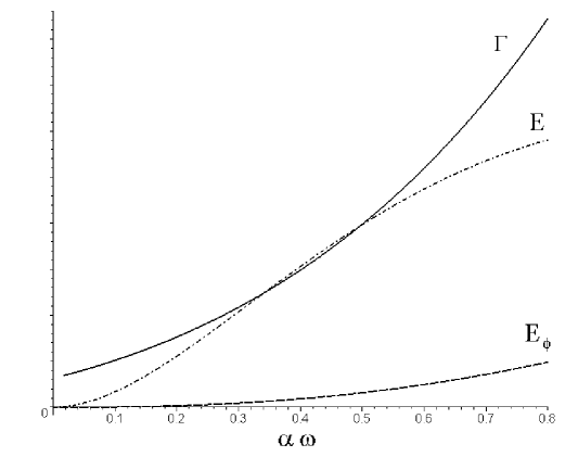
FIG. 2.: Qualitative behaviour of the energy flux $E_{\phi}$ carried by the dilaton waves generated at large distance by electromagnetic waves of energy $E$ for small values of $\alpha\,\bar{\omega}$ and $l=4$, $m=2$; $\Gamma$ is the ratio $(E_{\phi}/E)$. The vertical scale is arbitrary.

B Near horizon expansion

Near the horizon the energy flux (97) becomes singular on the threshold of super-radiance, therefore we shall only consider non-super-radiant modes. Since we also work in the small frequency approximation for the angular part of the wave modes, the expressions we obtain in this Section hold for

$${m\,\alpha\over 2\,M\,r_{+}}<\bar{\omega}<{1\over\alpha}\ .$$ (110)

For the dilaton waves in Eq. (95) one has

$$\left|T_{ij}\,\tilde{l}^{i}\,\tilde{l}^{j}\right|\simeq{1\over 2}\,\left(7\,\bar{\omega}^{2}-{11\,m\,\alpha\,\bar{\omega}\over 4\,M\,r_{+}}+{9\,m^{2}\,\alpha^{2}\over 8\,M^{2}\,r_{+}^{2}}\right)\,|\Phi^{out/in}|^{2}\ .$$ (111)

The energy flux for the impinging electromagnetic wave is

$$\left.{dE\over dt\,d\Omega}\right|_{+}={\bar{\omega}\over 8\,M\,r_{+}\,(\bar{\omega}-\bar{\omega}_{+})}\,{\Delta^{2}\over 2\,\pi}\,|\Phi_{0}|^{2}\ .$$ (112)

Hence the (local) ratio

$$\Gamma(r\sim r_{+})\equiv{dE_{\phi}^{out/in}\over dE^{in}}\ ,$$ (113)

follows as displayed in Fig. 3 where it appears that $\Gamma$ begins to increase as it approaches the super-radiant threshold.

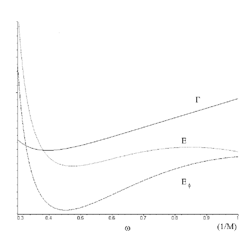
FIG. 3.: Qualitative behaviour of the energy flux $E_{\phi}$ carried by the dilaton waves generated near the horizon by electromagnetic waves of energy $E$ and frequency $\bar{\omega}$ (in units of $1/M$), $\alpha\sim M/2$ and $l=4$, $m=2$; $\Gamma$ is the ratio $(E_{\phi}/E)$. The vertical scale is arbitrary.

V Conclusion

In this paper we have analyzed the energy lost by the electromagnetic radiation emitted by a star to dilatonic waves on the background of a companion black hole. The expansion first introduced in [10] has once again been used to obtain separate expressions for the Maxwell scalars to first order in the charge-to-mass ratio $Q/M$. Our results apply to black holes with arbitrary angular momentum. We have obtained expressions for the amplitudes for the dilatonic waves generated by the incoming electromagnetic waves for large radial distances and near the horizon.

Explicit expressions for the angular part of the wave functions were obtained in the small $\alpha\,\omega$ limit by solving the recursion relations for the coefficients in the expansion of the spin-weighted spherical harmonics in terms of Jacobi polynomials. For the radial part of the wave functions we used the asymptotic expressions given in [15] at large distance. Near the horizon we improved the relation obtained in [15] by solving the radial wave equation to next to leading order in the distance from the horizon. The complete wave functions are products of the radial and angular parts at a fixed frequency. Thus the expressions we have obtained display the rate of energy loss as a function of the frequency of the incident electromagnetic radiation.

The results we have obtained for the energy loss to the dilatonic component of the gravitational field are qualitative because we have considered a simplified model of the true physical system. We assume, for example, that the observer is in the ecliptic plane and we ignore certain relativistic effects. However these results may prove to be a useful guide to future observers and should be taken into account when a detailed balance of all the effects occurring in the vicinity of a black hole is made and compared with the measurements. Such an analysis is a possible way of phenomenologically supporting or disproving the existence of a scalar (long range) component of gravity.

REFERENCES

[1]
J. Polchinski, String theory, Vol. 1 and 2,
Cambridge University Press, Cambridge (1998).
[2]
B. Harms and Y. Leblanc, Phys. Rev. D 46, 2334 (1992);
D 47, 2438 (1993).
[3]
B. Harms and Y. Leblanc, Ann. Phys. 244, 262 (1995);
244, 272 (1995).
[4]
P.H. Cox, B. Harms and Y. Leblanc, Europhys. Letts.
26, 321 (1994).
[5]
B. Harms and Y. Leblanc, Europhys. Letts. 27, 557 (1994).
[6]
B. Harms and Y. Leblanc, Ann. Phys. 242, 265 (1995).
[7]
B. Harms and Y. Leblanc,
Proceedings of the Texas/PASCOS Conference, 92.
Relativistic Astrophysics and Particle Cosmology,
eds. C.W. Ackerlof and M.A. Srednicki,
Annals of the New York Academy of Sciences 688, 454 (1993).
[8]
B. Harms and Y. Leblanc,
Supersymmetry and Unification of Fundamental Interactions,
ed. Pran Nath, World Scientific (1994) p.337.
[9]
B. Harms and Y. Leblanc,
Banff/CAP Workshop on Thermal Field Theory,
eds. F.C. Khanna, R. Kobes, G. Kunstatter and H. Umezawa,
World Scientific (1994), p.387.
[10]
R. Casadio, B. Harms, Y. Leblanc and P.H. Cox, Phys. Rev. D
55, 814 (1997).
[11]
We choose to work in the so called Einstein frame where
the Planck length (i.e., Newton’s constant) is a constant.
Other options are obtained by conformally rescaling the metric
and lead to a change in the value of the ADM mass, corresponding
to the fact that conformal mappings are canonical transformations
and change the canonical energy.
Comparison with the case of the string frame has been
investigated in detail in
R. Casadio and B. Harms, Charged dilatonic black holes:
string frame vs Einstein frame, gr-qc/9808026.
[12]
R. Casadio, B. Harms, Y. Leblanc and P.H. Cox, Phys. Rev. D 56
4948 (1997).
[13]
R. Casadio and B. Harms, Phys. Rev. D 58, 044015 (1998).
[14]
S. Chandrasekhar,
The Mathematical Theory of Black Holes,
Oxford University Press, Oxford (1983).
[15]
S.A. Teukolsky, Astroph. J. 185, 635 (1973).
[16]
C. T. Cunningham and J. M. Bardeen, Astroph. J. 183, 237
(1973);
G. Bao and E. Østgaard, Astroph. J. 443, 54 (1995).
[17]
E. Newman and R. Penrose, J. Math. Phys. 6, 566 (1964).
[18]
C. Flammer, Spheriodal Wave Functions,
Stanford University Press, Stanford (1957).
[19]
E. D. Fackerell and R. G. Crossman, J. Math. Phys. 18,
1849 (1977).
[20]
S. Mano, H. Suzuki and E. Takasugi, Prog. Theor. Phys. 95,
1079 (1996).
[21]
M. Abramowitz and I. Stegun, Handbook of Mathematical Functions,
Dover, N. Y. (1972).