gr-qc/9906024

Abstract

Local solutions of the static, spherically symmetric Einstein–Yang–Mills (EYM) equations with $SU(2)$ gauge group are studied on the basis of dynamical systems methods. This approach enables us to classify EYM solutions in the origin neighborhood, to prove the existence of solutions with the oscillating metric as well as the existence of local solutions for all known formal power series expansions, to study the extendibility of solutions, and to find two new local singular solutions.

PACS: 05.45.-a, 04.20.Ex, 04.60.m

 

^∗e-mail: zotov@eas.npi.msu.su

I INTRODUCTION

The discovery of a discrete family of asymptotically flat particle-like solutions for the static, spherically symmetric Einstein–Yang–Mills (EYM) equations with $SU(2)$ gauge group, made by Bartnik and McKinnon in 1988 [1], evoked considerable interest in these equations and their various generalizations. The intensity of investigations performed in this field is shown by the latest review [2], which summarizes a decade’s work and contains more than three hundred references to publications on the subject. However, there are still some problems which remain unsolved. One of the most interesting of these is probably the task to prove the existence of the metric oscillations in the origin, $r=0$, neighborhood, which were found numerically during the study of the EYM black holes interior structure [3]. The initial purpose of the present work was to solve this problem. Some other open questions can be found in [4].

Let us note that there are at least two approaches to the analysis of local solutions of nonlinear ordinary differential equations. One of them, namely, the asymptotic theory of differential equations, in some cases makes a possibility to obtain a complete classification of solutions in a singular point neighborhood. However, the right hand side of the studied equation must as a rule satisfy some rather specific conditions (see, e.g., [5]). Another way, known as the theory of dynamical systems, or the qualitative theory of differential equations, is less restrictive in this sense, though it also does not always lead to a comprehensive description of the solutions behavior (see, e.g., [6]). Nevertheless, there are a number of problems in astrophysics and cosmology, which were solved basing on this approach (see [7, 8] and references therein).

In this paper, dynamical systems methods are used for the analysis of the EYM solutions asymptotic behavior. This enables us to prove the existence of the above mentioned solutions with the oscillating metric, as well as the existence of local solutions for all known formal power series expansions, and to find two new local solutions. Moreover, a classification of local solutions in the vicinity of the origin is obtained. In particular, it is shown that there exists a neighborhood of $r=0$ such that the metric function has a fixed sign in it. Specifically, if the limiting value of the gauge function equals $\pm 1$, then all real solutions belong to the Schwarzschild and Bartnik–McKinnon type. In other cases, the solution behavior depends on the metric function sign. Namely, if the metric function is positive, then all solutions possess the behavior of the Reissner–Nordström type. If, on the contrary, the metric function is negative, then almost all solutions are such that the metric function oscillates with its amplitude growing unboundedly as $r\to 0$, but the gauge function is monotonous (though its derivative also oscillates with the unboundedly growing amplitude). Only particular solutions in this case exhibit asymptotic behavior of the “anti–Reissner–Nordström” type. This result also gives the negative answer to the question stated in [4], whether $r=0$ is a limit point for zeros of the metric function.

We have also considered the asymptotic behavior of solutions in the far field, $r\gg 1$, and in the vicinity of the points where the metric function tends to zero. This analysis leads to a discovery of two new local singular solutions and allows us to obtain some conclusions concerning the extendibility of solutions and their limiting behavior as the number of the gauge function nodes tends to infinity.

A detailed discussion of the physical interpretation of the EYM equations solutions can be found in [2].

II THE EQUATIONS

Recall that the space-time metric for the static, spherically symmetric EYM equations can be written as

$$ds^{2}=\sigma^{2}N\,dt^{2}-N^{-1}\,dr^{2}-r^{2}\left(d\vartheta^{2}+\sin^{2}\vartheta\,d\varphi^{2}\right),$$

where $N$ and $\sigma$ depend on $r$, and the Yang–Mills gauge field reads as

$$A=(T_{2}\,d\vartheta-T_{1}\sin\vartheta\,d\varphi)\,w+T_{3}\cos\vartheta\,d\varphi,$$

where $T_{i}=\frac{1}{2}\,\tau_{i}$ are the $SU(2)$ group generators and $\tau_{i}$ are the Pauli matrices, $i=1,2,3$ (see, e.g., [2]).

The EYM equations in this framework take the form of two ordinary differential equations for the metric function $N$ and the gauge function $w$:

$$\begin{split}&r^{3}N^{\prime}+\bigl{(}1+2{w^{\prime}}^{2}\bigr{)}r^{2}N+\left(1-w^{2}\right)^{2}-r^{2}=0,\\ &r^{3}Nw^{\prime\prime}-\left[\left(1-w^{2}\right)^{2}-r^{2}+r^{2}N\right]w^{\prime}+(1-w^{2})rw=0,\end{split}$$ (1)

and a decoupled equation for $\sigma$:

$$\frac{\sigma^{\prime}}{\sigma}=\frac{2{w^{\prime}}^{2}}{r}.$$

Since (1) do not involve $\sigma$, one can use these to obtain $N$ and $w$, and then solve the equation for $\sigma$. Thus we restrict our considerations to Eqs. (1). We also remark that (1) are invariant under the transformation $r\to-r$; thus, in what follows we discuss only the region $r\geq 0$.

For the purposes of studying the EYM solutions at finite $r$, it is convincing to rewrite (1) in terms of $w$ and $u=r^{2}N$. They become

$$\begin{split}&ru^{\prime}-\bigl{(}1-2{w^{\prime}}^{2}\bigr{)}u+\left(1-w^{2}\right)^{2}-r^{2}=0,\\[2.0pt] &ruw^{\prime\prime}-\left[u+\left(1-w^{2}\right)^{2}-r^{2}\right]w^{\prime}+\left(1-w^{2}\right)rw=0.\end{split}$$ (2)

Recall that the only known explicit solutions of (2) are the Schwarzschild solution

$$w\equiv\pm 1,\quad u=a\,r+r^{2},$$ (3)

and the Reissner–Nordström solution

$$w\equiv 0,\quad u=1+b\,r+r^{2},$$ (4)

where $a$ and $b$ are arbitrary constants.

In order to apply the theory of dynamical systems to the analysis of the EYM equations (2), it is necessary to write them as an autonomous system of first-order differential equations. Thus we introduce the function $v=w^{\prime}$ and an independent variable $t$ defined by $dr=ru\,dt$. After making these changes, we obtain the dynamical system

$$\begin{split}\dot{r}&=ru,\\ \dot{u}&=\left[\left(1-2v^{2}\right)u-\left(1-w^{2}\right)^{2}+r^{2}\right]u,\\ \dot{v}&=\left[u+\left(1-w^{2}\right)^{2}-r^{2}\right]v-\left(1-w^{2}\right)rw,\\ \dot{w}&=ruv.\end{split}$$ (5)

Notice that this system has solutions for $r\equiv 0$ and $u\equiv 0$, which do not take place for (2).

The first step to start analyzing (5) is to determine the critical points. It is easy to verify that the dynamical system (5) has the following critical sets:

$$\begin{array}[]{ll}\mathit{ARN}^{\pm}\colon&(0,-(1-w^{2})^{2},\pm 1,w),\\ \mathit{RN}\colon&(0,(1-w^{2})^{2},0,w),\\ \mathit{SBM}^{\pm}\colon&(0,0,v,\pm 1),\\ W\colon&(0,0,0,w),\\ \mathit{RH}\colon&(r,0,(1-w^{2})rw/[(1-w^{2})^{2}-r^{2}],w),\\ \mathit{DH}^{\pm}\colon&(\pm 1,0,v,0).\end{array}$$

All the critical sets belong to the hyperplanes $r=0$ and/or $u=0$, in which the conditions of the existence–uniqueness theorem do not hold for (2).

In what follows we shall not give a global phase portrait for (5), but we shall mainly concentrate on the results that have direct consequence for the EYM equations (2).

III PRELIMINARY INVESTIGATION OF THE
ORIGIN NEIGHBORHOOD

Let us consider the projection of (5) into the hyperplane $r=0$. This immediately leads to $w\equiv w_{0}=\mathrm{const}$. Thus the dynamical system (5) reduces to

$$\begin{split}\dot{u}&=-\alpha^{2}u+\left(1-2v^{2}\right)u^{2},\\ \dot{v}&=\alpha^{2}v+uv,\end{split}$$ (6)

where $\alpha=1-w_{0}^{2}$. Notice that (6) is invariant under the transformation $v\to-v$. Hence, the phase portrait will be symmetric with respect to the $u$-axis.

Since (6) contains a free parameter $\alpha$, it is convincing to split the analysis into two steps. Let us begin with $\alpha=0$. In this case, (6) reads as

$$\begin{split}&\dot{u}=\left(1-2v^{2}\right)u^{2},\\ &\dot{v}=uv.\end{split}$$ (7)

One can easily solve this system. First, the critical points, which are the projection of the sets $\mathit{SBM}^{\pm}$ and $W$, give $u\equiv 0$, $v\equiv\mathrm{const}$. Next,

$$C_{2}-C_{1}t=\frac{1}{v}\,e^{v^{2}}-2\int_{0}^{v}e^{\tilde{v}^{2}}\,d\tilde{v}=\frac{1}{v}\,e^{v^{2}}+i\sqrt{\pi}\,\operatorname{erf}(iv),\quad\text{and}\quad u=C_{1}v\,e^{-v^{2}},$$

where $C_{1}$ and $C_{2}$ are arbitrary constants, and $v\neq 0$. Finally, for $v\equiv 0$ one has $u=(C-t)^{-1}$, where $C$ is an arbitrary constant, $t\neq C$. We remark that if $u<0$, then the nontrivial solutions tend to zero as $t\to+\infty$. In the opposite case, they tend to zero as $t\to-\infty$. In particular, it follows that if $\lim_{r\to 0}w(r)=\pm 1$ for a solution of (2), then $\lim_{r\to 0}w^{\prime}(r)=0$.

The phase portrait of (7) is shown in Fig. 1.

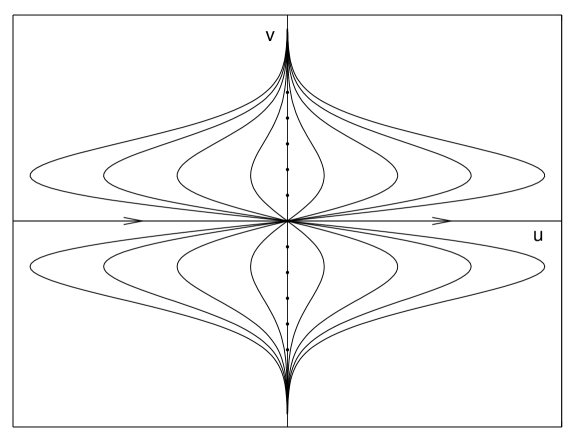
Figure 1: Phase portrait of the dynamical system (7).

Now let us study (6) for $\alpha\neq 0$ (i.e., for $w_{0}\neq\pm 1$). In this case, the system (6) has the following critical points: $Z$: $(0,0)$, $A^{\pm}$: $(-\alpha^{2},\pm 1)$, and $R$: $(\alpha^{2},0)$.

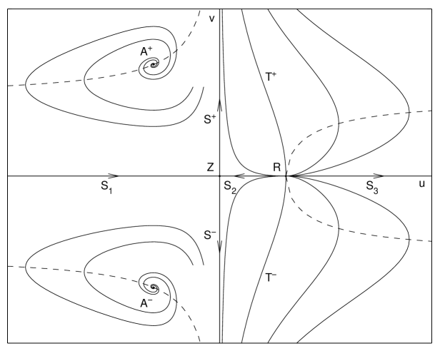
Figure 2: Phase portrait of the dynamical system (6) in the vicinity of the finite critical points for $\alpha\neq 0$. Dashed lines represent the curves $u^{\prime}(v)=0$.

The point $Z$ is the projection of $W$. The eigenvalues of $Z$ are $\lambda_{u}=-\alpha^{2}$ and $\lambda_{v}=\alpha^{2}$. Thus, $Z$ is a saddle. It has four separatrices, which can be easily obtained explicitly. The repelling separatrices, denote them by $S^{\pm}$ in accordance with the sign of $v$, are tangent to the eigenvector $\zeta_{v}=(0,1)$. They can be written as

$$u\equiv 0,\quad v=C_{v}\,e^{\alpha^{2}t}.$$ (8)

Here and forth the letter $C$, with an alphabetical subscript ($C_{u}$, $C_{v}$, etc.), denotes a nonzero constant.

The attracting separatrices are tangent to the eigenvector $\zeta_{u}=(1,0)$. They take the form

$$u=\frac{\alpha^{2}}{1+C_{u}\,e^{\alpha^{2}t}},\quad v\equiv 0.$$ (9)

One of these separatrices, denote it by $S_{1}$, belongs to the half-plane $u<0$. For $S_{1}$, $C_{u}<0$ and $t>-\alpha^{-2}\ln\lvert C_{u}\rvert$. Another separatrix, $S_{2}$, lies in the half-plane $u>0$. It has $C_{u}>0$ and joins $Z$ to $R$ (see Fig. 2).

The point $R$ is the projection of the critical curve $\mathit{RN}$. The eigenvalues of $R$ are $\lambda_{u}=\alpha^{2}$ and $\lambda_{v}=2\alpha^{2}$. Thus, it is an unstable node. Almost all trajectories that approach $R$ as $t\to-\infty$, are tangent to the eigenvector $\zeta_{u}=(1,0)$. The corresponding separatrices have the form (9). One of them, namely, $S_{2}$ joins $R$ to $Z$. Another one, $S_{3}$, is defined for $C_{u}<0$ and $t<-\alpha^{-2}\ln\lvert C_{u}\rvert$.

There are also two separatrices, denote them by $T^{\pm}$, which are tangent to the eigenvector $\zeta_{v}=(0,1)$. Let us show that they have the form

$$u=\alpha^{2}\left(1-\tfrac{2}{3}v^{2}\right)+o(v^{2})$$ (10)

as $v\to 0$. To see this, define $u_{v}=(u-\alpha^{2})v^{-1}$. Now the dynamical system (6) reads as

$$\begin{split}\dot{u}_{v}&=-\alpha^{2}\left(u_{v}+2\alpha^{2}v\right)-2\left(2\alpha^{2}+u_{v}v\right)u_{v}v^{2},\\ \dot{v}&=2\alpha^{2}v+u_{v}v^{2}.\end{split}$$

For $v=0$, this system has a saddle $(0,0)$ with the eigenvalues $\lambda_{u_{v}}=-\alpha^{2}$, $\lambda_{v}=2\alpha^{2}$ and the eigenvectors $\zeta_{u_{v}}=(1,0)$, $\zeta_{v}=\left(-\tfrac{2}{3}\alpha^{2},1\right)$. The separatrices that are tangent to the eigenvector $\zeta_{u_{v}}$, belong to the line $v=0$. Hence, there are no corresponding trajectories of (6). Conversely, the eigenvector $\zeta_{v}$ determines the outgoing separatrices, which take the form $u_{v}=-\tfrac{2}{3}\alpha^{2}v+o(v)$ as $v\to 0$. This yields (10).

Note that the same technique can be used to find the higher order terms in (10). This is also valid for the asymptotic solutions presented below.

Finally, the points $A^{\pm}$ represent projections of the critical curves $\mathit{ARN}^{\pm}$. The eigenvalues of $A^{\pm}$ are $\lambda_{u,v}=\frac{1}{2}\alpha^{2}(1\pm i\sqrt{15})$. Thus, these critical points are repelling foci. It is important to note here that for all the trajectories that spiral away from $A^{\pm}$, the metric function $u$ is strictly negative because of the separatrices $S^{\pm}$, and $v$ preserves its sign due to the separatrix $S_{1}$ (or, the same, because of the above mentioned invariance of (6) under the transformation $v\to-v$). Since there are no other finite critical points in the half-plane $u<0$, the trajectories that spiral away from the points $A^{\pm}$, do not have limit cycles. We remark that this can also be easily proved if we define the Dulac function for (6) by $(u^{2}v)^{-1}$. Hence, $u$ and $v$ exhibit oscillations with the amplitude growing infinitely as $t\to+\infty$.

Fig. 2 shows the phase portrait of (6) near the points $A^{\pm}$, $Z$, and $R$. Notice that this portrait is drastically different from that one shown in Fig. 1. Thus, $\alpha$ is a bifurcation parameter for the dynamical system (6).

In order to obtain the global phase portrait of (6), one has to study the behavior of its trajectories at infinity. Using the standard transform to the projective coordinates, one can find out that the system (6) has four critical points at the $(u,v)$ phase plane boundary, namely, $U^{\pm}$: $(u=\pm\infty,v=0)$ and $V^{\pm}$: $(u=0,v=\pm\infty)$. The points $U^{\pm}$ are saddles, and $V^{\pm}$ are saddle-nodes. The separatrices $S_{3}$ and $S_{1}$ are the only trajectories, which approach the points $U^{\pm}$ from the finite region of the phase plane. The points $V^{\pm}$, besides the separatrices $S^{\pm}$, have ingoing trajectories, which emanate from $R$. These trajectories have the form $u=\tfrac{1}{2}\alpha^{2}\,v^{-2}+o(v^{-2})$ as $v\to\infty$. The boundary of the phase plane contains two separatrices that join $U^{+}$ to $V^{\pm}$ and two separatrices that go from $V^{\pm}$ to $U^{-}$.

IV THE ORIGIN NEIGHBORHOOD

A The critical curves $\mathit{ARN}^{\pm}$

Let us turn to the analysis of the dynamical system (5) near the critical curves $\mathit{ARN}^{\pm}$: $(0,-(1-w^{2})^{2},\pm 1,w)$ for $w\neq\pm 1$. The excluded points also belong to the lines $\mathit{SBM}^{\pm}$ and will be studied below. Notice that the curves $\mathit{ARN}^{\pm}$ (with the points $w=\pm 1$ excluded) lie in the region $u<0$. Hence, in a neighborhood of these curves, $t$ growing to infinity corresponds to decreasing $r$ in the EYM equations (2).

The eigenvalues of $\mathit{ARN}^{\pm}$ are $\lambda_{r}=-(1-w^{2})^{2}$, $\lambda_{u,v}=\tfrac{1}{2}(1-w^{2})^{2}(1\pm i\sqrt{15})$, and $\lambda_{w}=0$. It should be recalled at this point that an $n$-dimensional critical set necessarily has $n$ zero eigenvalues (see, e.g., [7]). Thus, the zero eigenvalue $\lambda_{w}$ corresponds to the fact that $\mathit{ARN}^{\pm}$ are one-dimensional sets of critical points. Since other eigenvalues have nonzero real part, $\mathit{ARN}^{\pm}$ are hyperbolic sets.

The eigenvalues $\lambda_{u,v}$ determine three-dimensional unstable manifolds $M^{\pm}$ of the curves $\mathit{ARN}^{\pm}$, respectively. Since $\lambda_{u,v}$ are complex, the trajectories that lie on $M^{\pm}$, describe oscillatory behavior of $u$ and $v$. The found above trajectories that spiral away from the points $A^{\pm}$, are the projection of the trajectories that lie on $M^{\pm}$, in the plane $(r=0,w=w_{0}\neq\pm 1)$. The separatrices $S^{\pm}$ and $S_{1}$ do also have the obvious counterparts for (5):

$$r\equiv 0,\quad u\equiv 0,\quad v=C_{v}\,e^{\alpha^{2}t},\quad w\equiv w_{0},$$ (11)

and

$$r\equiv 0,\quad u=\frac{\alpha^{2}}{1+C_{u}\,e^{\alpha^{2}t}},\quad v\equiv 0,\quad w\equiv w_{0},$$ (12)

respectively, where $w_{0}=\mathrm{const}\neq\pm 1$, and $C_{u}<0$. These two-dimensional separatrices preserve the signs of $u$ and $v$ for the trajectories on $M^{\pm}$.

Recall that the trajectories that spiral away from $A^{\pm}$ do not have limit cycles. Evidently, the same is valid for the trajectories on $M^{\pm}$.

Next, due to the negative eigenvalue $\lambda_{r}$, each of the curves $\mathit{ARN}^{\pm}$ has two-dimensional stable separatrices, which are tangent to the eigenvectors

$$\zeta_{r}^{\pm}=\left(1,\pm 4(1-w^{2})w,\frac{w}{1-w^{2}},\pm 1\right),$$

where the upper sign applies for $\mathit{ARN}^{+}$ and the lower one for $\mathit{ARN}^{-}$. It is easy to see that these separatrices correspond to a one-parameter family of the EYM solutions that exist in the origin neighborhood. Thus, we conclude with

Proposition 1.

Let $\mathcal{U}^{-}$ be a set of solutions for the EYM equations (2) such that they are defined in some neighborhood of $r=0$, $u(r)<0$ in this neighborhood, and $\lim_{r\to 0}w(r)=w_{0}<\infty$, $w_{0}\neq\pm 1$. Then $\mathcal{U}^{-}$ is nonempty. Moreover, almost all solutions of (2) that belong to $\mathcal{U}^{-}$, are monotonous for the gauge function $w$ and oscillating for the metric function $u$. These solutions have the following properties:

1. The amplitude of the metric function oscillations grows unboundedly as $r\to 0$.

2. The values of the metric function at the points of maximum form a sequence, which monotonically converges to zero as $r\to 0$.

3. The derivative of the gauge function also oscillates with the amplitude growing unboundedly as $r\to 0$, and gets closer to zero on each cycle of the oscillations, but its sign remains unchanged.

Besides these solutions, $\mathcal{U}^{-}$ also contains a one-parameter family of local solutions of the “anti–Reissner–Nordström” type:

$$\begin{split}u&=-(1-w_{0}^{2})^{2}\pm 4(1-w_{0}^{2})w_{0}r+o(r),\\ w&=w_{0}\pm r+\frac{w_{0}}{2(1-w_{0}^{2})}\,r^{2}+o(r^{2})\end{split}$$ (13)

as $r\to 0$, where $w_{0}\neq\pm 1$.

Formal expansions of the form (13) and some corresponding numerical solutions were found in [3]. This paper was also the first to present the oscillating solutions. Some of their properties were analyzed in [9].

B The critical curve $\mathit{RN}$

Now let us study (5) in the vicinity of the curve $\mathit{RN}$: $(0,(1-w^{2})^{2},0,w)$ for $w\neq\pm 1$. Similar to the above, the excluded points also belong to the critical sets $\mathit{SBM}^{\pm}$ (and $W$) and will be studied below. Notice that $\mathit{RN}$ (with the points $w=\pm 1$ excluded) lies in the region $u>0$. Hence, in a neighborhood of $\mathit{RN}$, $t$ growing to infinity corresponds to increasing $r$ in the EYM equations (2).

The eigenvalues of $\mathit{RN}$ are $\lambda_{r}=\lambda_{u}=(1-w^{2})^{2}$, $\lambda_{v}=2(1-w^{2})^{2}$, and $\lambda_{w}=0$. Therefore, all trajectories of (5) in the vicinity of $\mathit{RN}$ belong to an unstable four-dimensional manifold; they correspond to a three-parameter family of EYM solutions.

The eigenvalue $\lambda_{v}$ determines two-dimensional separatrices, which are tangent to the eigenvector $\zeta_{v}=(0,0,1,0)$ and take the form

$$r\equiv 0,\quad w\equiv\mathrm{const}\neq\pm 1,\quad u=\alpha^{2}\left(1-\tfrac{2}{3}v^{2}\right)+o(v^{2})\quad\text{as }v\to 0.$$

The separatrices $T^{\pm}$ found above, represent their projection in the plane $(r=0,w=w_{0}\neq\pm 1)$. The EYM equations (2) do not have any corresponding solution. Conversely, the eigenvectors $\zeta_{r}=(1,0,w/(1-w^{2}),0)$ and $\zeta_{u}=(0,1,0,0)$ determine trajectories, which correspond to the EYM solutions

$$\begin{split}u&=(1-w_{0}^{2})^{2}+u_{1}r+o(r),\\ w&=w_{0}+\frac{w_{0}}{2(1-w_{0}^{2})}\,r^{2}+o(r^{2})\end{split}$$ (14)

as $r\to 0$, where $w_{0}\neq\pm 1$ and $u_{1}$ are arbitrary constants, and the higher order terms contain one more parameter.

Let us show how one can choose the third parameter in (14). The procedure will be similar to that one used for obtaining (10). Namely, consider (5) in the local coordinates

$$r,\quad u_{r}=\frac{u-(1-w^{2})^{2}}{r},\quad v_{r}=\frac{v}{r},\quad w.$$

Then the corresponding dynamical system, which we omit for brevity, has the critical surface $(0,u_{r},w/(1-w^{2}),w)$. (The other critical sets either have $w=\pm 1$ or do not belong to the hyperplane $r=0$.) The eigenvalues of this surface are $\lambda_{r}=\lambda_{v_{r}}=(1-w^{2})^{2}$ and $\lambda_{u_{r}}=\lambda_{w}=0$. It follows that all trajectories in a neighborhood of this surface belong to an unstable four-dimensional manifold. The nonzero eigenvalues have the eigenvectors $\zeta_{r}=(1,1+2w^{2},0,0)$ and $\zeta_{v_{r}}=(0,0,1,0)$. Thus, all the trajectories assume the form

$$u_{r}=u_{1}+(1+2w_{0}^{2})\,r+o(r),\quad v_{r}=\frac{w_{0}}{1-w_{0}^{2}}+v_{1}r+o(r),\quad w=w_{0}+o(r)$$

as $r\to 0$, where $w_{0}\neq\pm 1$, $u_{1}$, and $v_{1}$ are arbitrary constants. Changing back to the initial variables and taking into account the above discussion, one has

Proposition 2.

Let $\mathcal{U}^{+}$ be a set of solutions for the EYM equations (2) such that they are defined in some neighborhood of $r=0$, $u(r)>0$ in this neighborhood, and $\lim_{r\to 0}w(r)=w_{0}<\infty$, $w_{0}\neq\pm 1$. Then $\mathcal{U}^{+}$ is nonempty. Moreover, all solutions of (2) that belong to $\mathcal{U}^{+}$, form a three-parameter family of local solutions of the Reissner–Nordström type:

$$\begin{split}u&=(1-w_{0}^{2})^{2}+u_{1}r+r^{2}+o(r^{2}),\\ w&=w_{0}+\frac{w_{0}}{2(1-w_{0}^{2})}\,r^{2}+w_{3}r^{3}+o(r^{3})\end{split}$$ (15)

as $r\to 0$, where $w_{0}$, $u_{1}$ and $w_{3}$ are arbitrary constants, $w_{0}\neq\pm 1$.

A formal power series expansion (15) was presented in [10]. Some black hole solutions with this asymptotic were first found numerically in [3]. The local existence proof for these solutions was given in [11]. We remark that here we follow the terminology, introduced in [3], which is slightly different from that one used in [11] and [4].

C The critical lines $\mathit{SBM}^{\pm}$

The lines $\mathit{SBM}^{\pm}$: $(0,0,v,\pm 1)$ are degenerate critical sets, since the eigenvalues $\lambda_{r}$, $\lambda_{u}$, and $\lambda_{w}$ are equal to zero. In order to study the behavior of trajectories of (5) in a neighborhood of these lines, we use the standard technique [7].

First, define $\bar{w}$ by $w=\bar{w}\pm 1$, where the upper sign applies for $\mathit{SBM}^{+}$ and the lower one for $\mathit{SBM}^{-}$. Now the lines $\mathit{SBM}^{\pm}$ are transformed to the $v$-axis. Next, introduce the local coordinates

$$r_{u}=\frac{r}{u},\quad u,\quad v,\quad w_{u}=\frac{\bar{w}}{u},$$ (16)

in which the dynamical system (5) reads as

$$\begin{split}\dot{r}_{u}&=(2v^{2}+K)\,r_{u},\\ \dot{u}&=(1-2v^{2}-K)\,u,\\ \dot{v}&=(1+K)\,v+(1\pm uw_{u})(2\pm uw_{u})r_{u}uw_{u},\\ \dot{w}_{u}&=-(1-2v^{2}-K)\,w_{u}+r_{u}v,\\ \end{split}$$ (17)

where $K=[(2\pm uw_{u})^{2}w_{u}^{2}-r_{u}^{2}]u$, and an overdot stands for derivatives with respect to $\tau$ defined by $d\tau=u\,dt$ (thus, $\tau=\ln r+\mathrm{const}$).

The system (17) has one critical set in the hyperplane $u=0$, namely, the $r_{u}$-axis, which is an unstable hyperbolic line. The corresponding eigenvalues are $\lambda_{r_{u}}=0$, $\lambda_{u}=\lambda_{v}=1$, and $\lambda_{w_{u}}=-1$. The two-dimensional ingoing separatrices

$$r_{u}\equiv\mathrm{const}{},\quad u\equiv 0,\quad v\equiv 0,\quad w_{u}=C_{w}\,e^{-\tau},$$

which are tangent to the eigenvector $\zeta_{w_{u}}=(0,0,0,1)$, belong to the hyperplane $u=0$. Hence, they do not correspond to any trajectories of (5). In their turn, the eigenvalues $\lambda_{u}$ and $\lambda_{v}$, which have the eigenvectors $\zeta_{u}=(-r_{u}^{3},1,0,0)$ and $\zeta_{v}=(0,0,2,r_{u})$, determine the outgoing three-dimensional separatrices

$$r_{u}=r_{0}-r_{0}^{3}\,u+o(u),\quad v=2v_{1}\,u+o(u),\quad w_{u}=r_{0}v_{1}\,u+o(u)$$

as $u\to 0$, where $r_{0}$ and $v_{1}$ are arbitrary constants. This implies

Proposition 3.

All solutions of the EYM equations (2) such that $\lim_{r\to 0}w(r)=\pm 1$, belong to a two-parameter family of local solutions of the Schwarzschild type:

$$\begin{split}u&=u_{1}r+r^{2}+o(r^{2}),\\ w&=\pm 1+w_{2}r^{2}+o(r^{2})\end{split}$$ (18)

as $r\to 0$, where $u_{1}$ and $w_{2}$ are arbitrary constants.

In particular, these local solutions describe the behavior of the Bartnik–McKinnon particle-like solutions [1] (for $u_{1}=0$) and the black hole solutions of the Schwarzschild type [3] in the vicinity of the origin.

It is interesting to note that the separatrices that are tangent to the eigenvector $\zeta_{u}$, can be written as

$$u=\frac{1+u_{1}r_{u}}{r_{u}^{2}},\quad v\equiv 0,\quad w_{u}\equiv 0,$$

where $u_{1}$ is an arbitrary constant, and $r_{u}\neq 0$. Obviously, these separatrices correspond to the Schwarzschild solution (3).

We also remark that the coordinates (16) enable us to resolve the degeneracy of the $v$-axis along the $u$-direction. Analysis of the $r$- and $w$-directions leads to the same conclusion for the EYM equations as stated in Proposition 3.

It is necessary to underline here that we discuss only real EYM solutions, though the EYM equations also possess complex solutions. For example, a study of (5) in the local coordinates $(r,u/r^{2},v,\bar{w}/r)$, leads to a discovery of complex EYM solutions of the form

$$\begin{split}&u=-\left(1+4w_{1}^{2}\right)\left(r^{2}+w_{0}w_{1}r^{3}\right)+o(r^{3}),\\ \vskip 3.0pt plus 1.0pt minus 1.0pt&w=w_{0}+w_{1}r-\tfrac{1}{8}w_{0}r^{2}+o(r^{2})\end{split}$$

as $r\to 0$, where $w_{0}=\pm 1$ and $w_{1}=\pm(\sqrt{3}\pm i\sqrt{5})/4$. These solutions do not have free parameters.

D The critical line $W$

The eigenvalues of the critical line $W$: $(0,0,0,w)$ are $\lambda_{r}=0$, $\lambda_{u}=-(1-w^{2})^{2}$, $\lambda_{v}=(1-w^{2})^{2}$, and $\lambda_{w}=0$. Hence, $W$ is degenerate for any $w$. The eigenvalues $\lambda_{u}$ and $\lambda_{v}$ are nonzero and have different signs whenever $w\neq\pm 1$. In this case, $W$ is an unstable critical set with the outgoing two-dimensional separatrices (11) and the ingoing two-dimensional separatrices (12). Investigation of (5) in the vicinity of $W$ gives the same result for the EYM equations as already stated in Proposition 3. By this reason we omit the discussion.

Thus, we have obtained a description of the EYM solutions that have finite values of the gauge function $w$ in the origin neighborhood. It follows from our considerations that for all these solutions $\lim_{r\to 0}w(r)=w_{0}<\infty$. A standard analysis of the dynamical system (5) in the projective coordinates $(rz,uz,vz,z=1/w)$ reveals that Eqs. (2) do not have solutions such that $\lim_{r\to 0}w(r)=\infty$. Hence, the results of this section can be summarized in the following classification of the EYM solutions, defined in the vicinity of the origin.

Theorem.

All real solutions of the EYM equations (2), defined in a neighborhood of $r=0$, belong to one of the following disjoint classes:

1. $w_{0}=\pm 1$. In this case, all solutions are of the Schwarzschild and Bartnik–McKinnon type (18).

2. $w_{0}\neq\pm 1$, and the metric function $u$ is negative in some neighborhood of $r=0$. In this case, almost all solutions are such that the metric function oscillates with the unboundedly growing amplitude as $r\to 0$, but the gauge function is monotonous (though its derivative also oscillates with the amplitude growing infinitely). Only particular solutions in this case exhibit asymptotic behavior of the “anti–Reissner–Nordström” type (13).

3. $w_{0}\neq\pm 1$, and the metric function $u$ is positive in some neighborhood of $r=0$. In this case, all solutions belong to the Reissner–Nordström type (15).

We remark that this classification scheme explains why almost all interior black hole solutions, found numerically in [3], exhibit oscillatory behavior of the metric.

V CRITICAL SETS FOR $r\neq 0$

A The critical surface $\mathit{RH}$

Now let us discuss the remaining critical sets of (5). The surface $\mathit{RH}$: $(r,0,(1-w^{2})rw/[(1-w^{2})^{2}-r^{2}],w)$ is an unstable hyperbolic set. The eigenvalues of $\mathit{RH}$ are $\lambda_{r}=0$, $\lambda_{u}=-[(1-w^{2})^{2}-r^{2}]$, $\lambda_{v}=(1-w^{2})^{2}-r^{2}$, and $\lambda_{w}=0$. The three-dimensional separatrices that are tangent to the eigenvector $\zeta_{v}=(0,0,1,0)$ read as

$$r\equiv r_{0}=\mathrm{const}{},\quad u\equiv 0,\quad v=\frac{\gamma}{\beta}+C_{v}\,e^{\beta t},\quad w\equiv w_{0}=\mathrm{const}{},$$

where $\beta=(1-w_{0}^{2})^{2}-r_{0}^{2}\neq 0$ and $\gamma=(1-w_{0}^{2})r_{0}w_{0}$. Obviously, they do not correspond to any EYM solution. In their turn, the three-dimensional separatrices that are tangent to the eigenvector

$$\zeta_{u}=\left(1,-\frac{G}{r},\frac{\{2F^{4}-[F^{3}+(1-3w^{2})r^{2}]r^{2}\}Fw}{2G^{3}},\frac{Frw}{G}\right),$$

where $F=1-w^{2}$ and $G=F^{2}-r^{2}$, correspond to a two-parameter family of local EYM solutions. It is convenient to fix one of these parameters and to write down these solutions as follows.

Proposition 4.

For any fixed $r_{h}>0$, the EYM equations (2) possess a one-parameter family of local solutions of the form

$$\begin{split}u&=-\frac{(1-w_{h}^{2})^{2}-r_{h}^{2}}{r_{h}}\,s+o(s),\\[5.69054pt] w&=w_{h}+\frac{(1-w_{h}^{2})r_{h}w_{h}}{(1-w_{h}^{2})^{2}-r_{h}^{2}}\,s\\[5.69054pt] &\quad\,+\frac{(1-w_{h}^{2})\{2(1-w_{h}^{2})^{4}-[(1-w_{h}^{2})^{3}+(1-3w_{h}^{2})r_{h}^{2}]r_{h}^{2}\}w_{h}}{4[(1-w_{h}^{2})^{2}-r_{h}^{2}]^{3}}\,s^{2}+o(s^{2})\\[5.69054pt] \end{split}$$ (19)

as $s=r-r_{h}\to 0$, where $w_{h}$ is a constant, satisfying $\lvert 1-w_{h}^{2}\rvert\neq r_{h}$.

The local solutions (19) represent the EYM solutions in the vicinity of a regular horizon. For the black hole solutions, this is either an event horizon (if $r_{h}>\lvert 1-w_{h}^{2}\rvert$), or an interior Cauchy horizon (if $r_{h}<\lvert 1-w_{h}^{2}\rvert$). The first existence proof for these local solutions was given in [12]. Some black hole solutions with an interior horizon were found numerically in [3].

Note that $\mathit{RH}$ transforms to the line $W$ for $r=0$.

B The critical lines $\mathit{DH}^{\pm}$

The lines $\mathit{DH}^{\pm}$: $(\pm 1,0,v,0)$ are degenerate. All their eigenvalues are equal to zero. Since the EYM equations (2) are invariant under the transformation $r\to-r$, we shall study (5) only in the vicinity of the line $\mathit{DH}^{+}$.

It is convenient to use the local coordinates

$$\bar{r}=r-1,\quad u_{r}=\frac{u}{\bar{r}^{2}},\quad v,\quad w_{r}=\frac{w}{\bar{r}},$$

in which the dynamical system (5) reads as

$$\begin{split}\dot{\bar{r}}&=(1+\bar{r})\,\bar{r}u_{r},\\ \dot{u}_{r}&=\left[2-\left(2+\bar{r}+2\bar{r}v^{2}\right)u_{r}+\left(1+2w_{r}^{2}\right)\bar{r}-\bar{r}^{3}w_{r}^{4}\right]u_{r},\\ \dot{v}&=-2v-w_{r}-\left(v+w_{r}-u_{r}v+2vw_{r}^{2}\right)\bar{r}+\bar{r}^{2}w_{r}^{3}+(1+vw_{r})\bar{r}^{3}w_{r}^{3},\\ \dot{w}_{r}&=(1+\bar{r})(v-w_{r})\,u_{r},\end{split}$$ (20)

where an overdot stands for derivatives with respect to $\tau$ defined by $d\tau=\bar{r}\,dt$.

There are two critical sets of (20) in the hyperplane $\bar{r}=0$, namely, the point $D$: $(0,1,0,0)$ and the line $L$: $(0,0,-\frac{1}{2}w_{r},w_{r})$. The eigenvalues of $D$ are $\lambda_{\bar{r}}=1$, $\lambda_{u_{r}}=-2$, and $\lambda_{v,w_{r}}=-\tfrac{1}{2}(3\pm i\sqrt{3})$. Thus, $D$ is a saddle. The outgoing one-dimensional separatrices

$$\bar{r}=-\frac{1}{1+C_{r}\,e^{-\tau}},\quad u_{r}\equiv 1,\quad v\equiv 0,\quad w_{r}\equiv 0,$$

which are tangent to the eigenvector $\zeta_{\bar{r}}=(1,0,0,0)$, correspond to the extreme Reissner–Nordström solution

$$w\equiv 0,\quad u=(1-r)^{2}.$$ (21)

Besides this, in the vicinity of $D$ there exists a stable three-dimensional manifold. In order to figure out whether this manifold belongs to the hyperplane $\bar{r}=0$, one may study a projection of (20) into $\bar{r}=\mathrm{const}$. It occurs that the critical point $(1,0,0)$ exists for any $\bar{r}$ and has the eigenvalues $\lambda_{u_{r}}=-2-\bar{r}$ and $\lambda_{v,w_{r}}=-\frac{1}{2}\,(3+\bar{r})\pm i\sqrt{(3+\bar{r})(1+3\bar{r})}$. Hence, for any $\bar{r}>-1/3$ all the eigenvalues have negative real part, and $\lambda_{v}$ and $\lambda_{w_{r}}$ are complex conjugate. Thus, the stable three-dimensional manifold does not belong to the hyperplane $\bar{r}=0$, and the trajectories on this manifold correspond to a two-parameter family of local EYM solutions.

It is interesting to note that the projection of (20) into the plane $(\bar{r}=0,u_{r}=1)$ gives a system of two linear differential equations

$$\begin{split}\dot{v}&=-2v-w_{r},\\ \dot{w}_{r}&=v-w_{r},\end{split}$$ (22)

which can be easily solved:

$$\begin{split}v&=\left[C_{1}\cos\left(\tfrac{\sqrt{3}}{2}\tau\right)-\tfrac{\sqrt{3}}{3}(C_{1}+2C_{2})\sin\left(\tfrac{\sqrt{3}}{2}\tau\right)\right]\,\exp\left(-\tfrac{3}{2}\tau\right),\\ w_{r}&=\left[C_{2}\cos\left(\tfrac{\sqrt{3}}{2}\tau\right)+\tfrac{\sqrt{3}}{3}(2C_{1}+C_{2})\sin\left(\tfrac{\sqrt{3}}{2}\tau\right)\right]\,\exp\left(-\tfrac{3}{2}\tau\right),\end{split}$$

where $C_{1}$ and $C_{2}$ are the constants of integration. Thus, the projection of (20) into $(\bar{r}=0,u_{r}=1)$ represents linear oscillations of $v$ and $w_{r}$ with infinitely many zeros.

It is easy to see that $\bar{r}\to 0$ corresponds to $\tau\to-\infty$, so that $w^{\prime}$ diverges as $r\to 1$. Conversely, $r$ goes away from $1$ as $\tau\to+\infty$, and these solutions tend to the extreme Reissner–Nordström solution. Thus, we have

Proposition 5.

There exists a neighborhood of $r=1$, in which the EYM equations (2) have a two-parameter family of local solutions with the gauge function oscillating with infinitely many zeros, and the metric function tending to zero.

These solutions can be treated as a description of the limiting behavior of the EYM solutions in the vicinity of $r=1$ as the number of the gauge function nodes tends to infinity. The limiting behavior of the EYM solutions was first studied in [13, 14, 15]. Solutions that exhibit oscillations of $w$ were first discussed in [16]. But, in addition to the results of [16], we see that the gauge function may have infinitely many zeros not only to the left of $r=1$, but also to the right.

Finally, the line $L$ has the eigenvalues $\lambda_{\bar{r}}=0$, $\lambda_{u_{r}}=2$, $\lambda_{v}=-2$, and $\lambda_{w_{r}}=0$. Thus, $L$ is a degenerate set. The eigenvectors $\zeta_{u_{r}}=(0,1,\frac{3}{16}w_{r},-\frac{3}{4}w_{r})$ and $\zeta_{v}=(0,0,1,0)$ determine two-dimensional separatrices, which lie in the hyperplane $\bar{r}=0$. Thus, they do not correspond to any EYM solution. Further investigation of the line $L$ did not reveal any trajectories of (5) that have corresponding EYM solutions different from the discussed above.

VI SOLUTIONS WITH A SINGULAR HORIZON

A typical EYM solution cannot be continued to the far field, since it has a singular horizon, i.e., a point, at which the metric function tends to zero, the gauge functions stays finite, but its derivative diverges [17, 12]. This fact was first noticed in [13], and a power series expansion, describing the behavior of the EYM solutions in the vicinity of a singular horizon was given. Let us show how one can obtain singular EYM solutions basing on dynamical systems methods. This will also lead us to a discovery of two new local solutions.

Let us rewrite the dynamical system (5) as

$$\begin{split}\dot{r}&=ruz^{2},\\ \dot{u}&=-\left[\left(2-z^{2}\right)u+\left(1-w^{2}\right)^{2}z^{2}-r^{2}z^{2}\right]u,\\ \dot{z}&=-\left[u+\left(1-w^{2}\right)^{2}-r^{2}-\left(1-w^{2}\right)rzw\right]z^{3},\\ \dot{w}&=ruz,\end{split}$$ (23)

where $z=1/v$, and an overdot stands for derivatives with respect to $\tau$ defined by $dt=z^{2}\,d\tau$.

For $z=0$, the critical points of (23) form a degenerate plane $(r,0,0,w)$. In order to study (23) in the vicinity of this plane, we introduce the local coordinates $(r,u_{z}=u/z^{2},z,w)$, in which (23) can be written as

$$\begin{split}\dot{r}&=ru_{z}z^{2},\\ \dot{u}_{z}&=-\left[\left(2-3z^{2}\right)u_{z}-\left(1-w^{2}\right)^{2}+r^{2}+2\left(1-w^{2}\right)rzw\right]u_{z},\\ \dot{z}&=-\left[u_{z}z^{2}+\left(1-w^{2}\right)^{2}-r^{2}-\left(1-w^{2}\right)rzw\right]z,\\ \dot{w}&=ru_{z}z,\end{split}$$ (24)

where an overdot stands for derivatives with respect to $t$.

The system (24) has two critical sets in the hyperplane $z=0$, namely, the plane $RW_{1}$: $(r,0,0,w)$ and the surface $\mathit{SH}$: $(r,[(1-w^{2})^{2}-r^{2}]/2,0,w)$, which are nondegenerate whenever

$$r\neq\lvert 1-w^{2}\rvert.$$ (25)

The eigenvalues of $RW_{1}$ are $\lambda_{r}=0$, $\lambda_{u_{z}}=(1-w^{2})^{2}-r^{2}$, $\lambda_{z}=-\lambda_{u_{z}}$, and $\lambda_{w}=0$. Thus, $RW_{1}$ is an unstable hyperbolic set. One can easily see that if (25) holds, then the eigenvectors $\zeta_{u_{z}}=(0,1,0,0)$ and $\zeta_{z}=(0,0,1,0)$ determine the three-dimensional separatrices

$$r\equiv r_{0}=\mathrm{const}{},\quad u_{z}=\frac{\beta}{2+C_{u}\,e^{-\beta t}},\quad z\equiv 0,\quad w\equiv w_{0}=\mathrm{const}{},$$

and

$$r\equiv r_{0},\quad u_{z}\equiv 0,\quad z=\frac{\beta}{\gamma+C_{z}\,e^{\beta t}},\quad w\equiv w_{0},$$

respectively, where $\beta=(1-w_{0}^{2})^{2}-r_{0}^{2}\neq 0$ and $\gamma=(1-w_{0}^{2})r_{0}w_{0}$. Clearly, these separatrices do not correspond to any EYM solution.

Next, the eigenvalues of $\mathit{SH}$ are $\lambda_{r}=0$, $\lambda_{u_{z}}=\lambda_{z}=-[(1-w^{2})^{2}-r^{2}]$, and $\lambda_{w}=0$. Hence, if (25) holds, then all trajectories of (24) in the vicinity of $\mathit{SH}$ belong to a four-dimensional manifold. The eigenvalues $\lambda_{u_{z}}$ and $\lambda_{z}$ have the eigenvectors $\zeta_{u_{z}}=(0,1,0,0)$ and $\zeta_{z}=(0,0,1,-\frac{1}{2}r)$. Thus, all trajectories in the vicinity of $\mathit{SH}$ take the form

$$r=r_{0}+o(z),\quad u_{z}=\frac{\beta}{2}+u_{1}z+o(z),\quad w=w_{0}-\frac{r_{0}}{2}z+o(z)\quad$$

as $z\to 0$, where $\beta\neq 0$, and $u_{1}$ is an arbitrary constant. This leads to

Proposition 6.

Let $r_{0}>0$ be a point such that

$$\lim_{r\to r_{0}}u(r)=0,\quad\lim_{r\to r_{0}}w(r)=w_{0}<\infty,\quad\lim_{r\to r_{0}}w^{\prime}(r)=\infty,$$

and $\beta=(1-w_{0}^{2})^{2}-r_{0}^{2}\neq 0$. Then all solutions of the EYM equations (2) in the vicinity of $r_{0}$ have the form

$$u=\frac{2\beta}{r_{0}}s^{2}+u_{1}s^{3}+o(s^{3}),\quad w=w_{0}\pm\sqrt{r_{0}}\,s+o(s)$$ (26)

as $s=\sqrt{r_{0}-r}\to 0$, where $u_{1}$ is an arbitrary constant. These solutions do not have other parameters besides $w_{0}$ and $u_{1}$.

Thus, local solutions (26) exist in the vicinity of any point $r_{0}>0$, $r_{0}\neq\lvert 1-w_{0}^{2}\rvert$.

Notice that solutions (19) were determined by the trajectories that belong to a three-dimensional manifold. Unlike them, singular solutions (26) correspond to the trajectories that lie on a four-dimensional manifold. It follows immediately that in the vicinity of an arbitrary point $r_{0}>0$ such that $\lim_{r\to r_{0}}u(r)=0$, $\lim_{r\to r_{0}}w(r)=w_{0}$, and $r_{0}\neq\lvert 1-w_{0}^{2}\rvert$, almost all solutions of the EYM equations (2) exhibit asymptotic behavior (26) and, therefore, cannot be continued toward $r=\infty$.

Let us also mention that it follows from (26) and the above analysis of the critical sets $\mathit{RH}$ and $\mathit{DH}^{\pm}$ that almost all EYM solutions, defined at an arbitrary finite point $r_{0}>0$, can be continued to the left for all $r<r_{0}$. A detailed investigation of extendibility of solutions of the EYM equations can be found in [4].

Now let us study (23) in the vicinity of the curve $r=\lvert 1-w^{2}\rvert$. We start with $\lvert w\rvert\leq 1$. In the local coordinates

$$r_{z}=\frac{1}{z}\,(r-1+w^{2}),\quad u_{z}=\frac{u}{z^{3}},\quad z,\quad w,$$

the dynamical system (23) reads as

$$\begin{split}\dot{r}_{z}&=\left(1-w^{2}\right)\bigl{(}z+2w\bigr{)}u_{z}+\left[2(z+w)u_{z}z-\left(1-w^{2}\right)^{2}w\right]r_{z}\\ &\quad\,-\left(1-w^{2}\right)\bigl{(}2+zw\bigr{)}r_{z}^{2}-r_{z}^{3}z,\\ \dot{u}_{z}&=-\left[2\left(1-2z^{2}\right)u_{z}+3\left(1-w^{2}\right)^{2}w+\left(1-w^{2}\right)\bigl{(}4+3zw\bigr{)}r_{z}+2r_{z}^{2}z\right]u_{z},\\ \dot{z}&=\left[\left(1-w^{2}\right)^{2}w-u_{z}z^{2}+\left(1-w^{2}\right)\bigl{(}2+zw\bigr{)}r_{z}+r_{z}^{2}z\right]z,\\ \dot{w}&=\left(1-w^{2}+r_{z}z\right)u_{z}z,\end{split}$$ (27)

where an overdot stands for derivatives with respect to $\tau$ defined by $d\tau=z\,dt$.

The system (27) has six critical sets in the hyperplane $z=0$, namely, $\mathit{LW}$: $(0,0,0,w)$, $\mathit{LR}^{\pm}$: $(r_{z},0,0,\pm 1)$, $\mathit{CR}$: $(-\tfrac{1}{2}(1-w^{2})w,0,0,w)$, $RU_{1}$: $(-(1-w^{2})w,\tfrac{1}{2}(1-w^{2})^{2}w,0,w)$, and $RU_{2}$: $(-\tfrac{3}{2}(1-w^{2})w,\tfrac{3}{2}(1-w^{2})^{2}w,0,w)$. Analysis of the first four critical sets does not reveal any trajectories of (27) that have corresponding EYM solutions. Thus we discuss only the curves $RU_{1}$ and $RU_{2}$.

The eigenvalues of $RU_{1}$ are $\lambda_{r_{z}}=\lambda_{u_{z}}=(1-w^{2})^{2}w$, $\lambda_{z}=-(1-w^{2})^{2}w$, and $\lambda_{w}=0$. Thus, $RU_{1}$ is an unstable hyperbolic critical set whenever

$$w\neq 0,\pm 1.$$ (28)

In this case, all trajectories on a three-dimensional manifold, determined by $\lambda_{r_{z}}$ and $\lambda_{u_{z}}$, are tangent to the eigenvector $\zeta_{r_{z},u_{z}}=(1,-(1-w^{2}),0,0)$, which defines the two-dimensional separatrices

$$u_{z}=-\tfrac{1}{2}\alpha^{2}w_{0}-\alpha r_{z},\quad z\equiv 0,\quad w\equiv w_{0}\neq 0,\pm 1.$$

One of these separatrices joins $RU_{1}$ to $\mathit{CR}$. However, the hole manifold belongs to the hyperplane $z=0$. Thus, the trajectories on it do not correspond to any EYM solution.

Unlike this, the two-dimensional separatrices that are tangent to the eigenvector

$$\zeta_{z}=\left(\tfrac{1}{8}\,\left(1-w^{2}\right)\left(3-5w^{2}\right),-\tfrac{1}{4}\,\left(1-w^{2}\right)^{2}\left(2-3w^{2}\right),1,-\tfrac{1}{2}\,\left(1-w^{2}\right)\right),$$

take the form

$$\begin{split}r_{z}&=-\alpha w_{0}+\tfrac{1}{8}\,\alpha\left(3-5w_{0}^{2}\right)z+o(z),\\ u_{z}&=\tfrac{1}{2}\,\alpha^{2}w_{0}-\tfrac{1}{4}\,\alpha^{2}\left(2-3w_{0}^{2}\right)z+o(z),\\ w&=w_{0}-\tfrac{1}{2}\,\alpha z+o(z)\end{split}$$ (29)

as $z\to 0$, where $w_{0}\neq 0,\pm 1$, and thus have corresponding EYM solutions.

Finally, the eigenvalues of $RU_{2}$ are $\lambda_{r_{z}}=-(1-w^{2})^{2}w$, $\lambda_{u_{z}}=3(1-w^{2})^{2}w$, $\lambda_{z}=-2(1-w^{2})^{2}w$, and $\lambda_{w}=0$. Hence, $RU_{2}$ is also an unstable hyperbolic critical set whenever (28) holds. The eigenvector $\zeta_{u_{z}}=(1,-(1-w^{2}),0,0)$ defines the two-dimensional separatrices

$$u_{z}=-\alpha r_{z},\quad z\equiv 0,\quad w\equiv w_{0}\neq 0,\pm 1.$$

One of them joins $RU_{2}$ to $\mathit{LW}$. Besides these separatrices, there is also a three-dimensional manifold, defined by the eigenvalues $\lambda_{r_{z}}$ and $\lambda_{z}$. Almost all trajectories on this manifold are tangent to the eigenvector $\zeta_{r_{z}}=(1,-3(1-w^{2}),0,0)$, which determines the separatrices

$$u_{z}=\tfrac{3}{2}\,\alpha^{2}w_{0}-3\alpha s+o(s)\quad\text{as }s=r_{z}+\tfrac{3}{2}\,\alpha w_{0}\to 0,\qquad z\equiv 0,\quad w\equiv w_{0},$$

where $w_{0}\neq 0,\pm 1$. In addition, there exist two-dimensional separatrices, which are tangent to the eigenvector

$$\zeta_{z}=\left(\tfrac{3}{40}\,\left(1-w^{2}\right)\left(13-12w^{2}\right),-\tfrac{9}{40}\,\left(1-w^{2}\right)^{2}\left(11-9w^{2}\right),1,-\tfrac{3}{4}\,\left(1-w^{2}\right)\right)$$

and take the form

$$\begin{split}r_{z}&=-\tfrac{3}{2}\,\alpha w_{0}+\tfrac{3}{40}\,\alpha\left(13-12w_{0}^{2}\right)z+o(z),\\ u_{z}&=\tfrac{3}{2}\,\alpha^{2}w_{0}-\tfrac{9}{40}\,\alpha^{2}\left(11-9w_{0}^{2}\right)z+o(z),\\ w&=w_{0}-\tfrac{3}{4}\,\alpha z+o(z)\end{split}$$ (30)

as $z\to 0$, where $w_{0}\neq 0,\pm 1$. These separatrices, together with (29), have corresponding singular EYM solutions. Conversely, all trajectories, defined by the eigenvalues $\lambda_{u_{z}}$ and $\lambda_{r_{z}}$, belong to the hyperplane $z=0$ and do not have counterparts neither for the dynamical system (23), nor for the EYM equations.

Analysis of (23) in the vicinity of the curve $r=-(1-w^{2})$ for $\lvert w\rvert\geq 1$ is completely analogous to the previous case. The dynamical system (23), written in the local coordinates

$$r_{z}=\frac{1}{z}\,(r+1-w^{2}),\quad u_{z},\quad z,\quad w,$$

has the same critical sets in the hyperplane $z=0$, as (27), to the exclusion of the curves $RU_{1}$ and $RU_{2}$, which in this case have the opposite sign of $u_{z}$. Asymptotic formulas (29) and (30) convert to

$$r_{z} =-\alpha w_{0}-\tfrac{1}{8}\,\alpha\left(3-5w_{0}^{2}\right)z+o(z),$$

$$u_{z} =-\tfrac{1}{2}\,\alpha^{2}w_{0}-\tfrac{1}{4}\,\alpha^{2}\left(2-3w_{0}^{2}\right)z+o(z),$$

$$w =w_{0}+\tfrac{1}{2}\,\alpha z+o(z),$$

and

$$r_{z} =-\tfrac{3}{2}\,\alpha w_{0}-\tfrac{3}{40}\,\alpha\left(13-12w_{0}^{2}\right)z+o(z),$$

$$u_{z} =-\tfrac{3}{2}\,\alpha^{2}w_{0}-\tfrac{9}{40}\,\alpha^{2}\left(11-9w_{0}^{2}\right)z+o(z),$$

$$w =w_{0}+\tfrac{3}{4}\,\alpha z+o(z)$$

as $z\to 0$, respectively. Recall that $\alpha=1-w_{0}^{2}=-r_{0}\neq 0,1$ here. Combining these solutions with (29) and (30), we get

Proposition 7.

In the vicinity of any point $r_{0}>0$, $r_{0}\neq 1$, the EYM equations (2) have solutions of the form

$$u=\pm 4\xi\sqrt{r_{0}}\,w_{0}\,s^{3}+O(s^{4}),\quad w=w_{0}\pm\sqrt{r_{0}}\,s+o(s),$$

and

$$u=\pm\frac{16}{3}\,\xi w_{0}w_{12}\,s^{3}+O(s^{4}),\quad w=w_{0}\pm w_{12}\,s+o(s),$$

as $s=\sqrt{r_{0}-r}\to 0$, where $r_{0}=\lvert 1-w_{0}^{2}\rvert$, $\xi=-\operatorname{sgn}(1-w_{0}^{2})$, and $w_{12}=\sqrt{3r_{0}/2}$. These solutions do not have free parameters.

To the best of the author’s knowledge, the presented local solutions are new.

Notice that Proposition 7 excludes the cases $r_{0}=1$ and $r_{0}=0$, which correspond to $w_{0}=0,\pm 1$. Analysis of the first one reveals complex solutions of the EYM equations. We do not discuss them here, since their physical interpretation is unclear. The latter case has already been discussed in Sec. IV.

VII SOLUTIONS IN THE FAR FIELD

The behavior of the EYM solutions in the far field, $r\gg 1$, was studied in great details, see [18] and references therein. In this section, we briefly give another existence proof for the asymptotically flat solutions and obtain a description of the limiting behavior of the EYM solutions as the number of the gauge function nodes tends to infinity. To implement this task, we return to the EYM equations (1), but we change $r$ to $z=1/r$. Next, we rewrite (1) as a dynamical system of the form

$$\begin{split}\dot{z}&=z^{2}N,\\ \dot{N}&=\left[-1+\left(1+2z^{4}v^{2}\right)N+\left(1-w^{2}\right)^{2}z^{2}\right]zN,\\ \dot{v}&=\left[1-3N-\left(1-w^{2}\right)^{2}z^{2}\right]zv-\left(1-w^{2}\right)w,\\ \dot{w}&=z^{2}vN,\end{split}$$ (31)

where $v=w^{\prime}(z)$, and an overdot stands for derivatives with respect to  $t$ defined by $dz=z^{2}N\,dt$.

The dynamical system (31) has two critical sets in the hyperplane $z=0$, namely, the planes $\mathit{AF}^{\pm}$: $(0,N,v,\pm 1)$ and $\mathit{OS}$: $(0,N,v,0)$. Both of them are degenerate. Thus we perform the standard procedure of their investigation for finite $N$ and $v$.

A The critical planes $\mathit{AF}^{\pm}$

In this case, we introduce the local coordinates $(z,N,v,w_{z}=\bar{w}/z)$, where $w=\bar{w}\pm 1$; here the upper sign applies for $\mathit{AF}^{+}$ and the lower one for $\mathit{AF}^{-}$. Now (31) can be written as

$$\begin{split}\dot{z}&=zN,\\ \dot{N}&=\left[-1+\left(1+2z^{4}v^{2}\right)N+(2\pm zw_{z})^{2}z^{4}w_{z}^{2}\right]N,\\ \dot{v}&=\left[1-3N-(2\pm zw_{z})^{2}z^{4}w_{z}^{2}\right]v+(1\pm zw_{z})(2\pm zw_{z})w_{z},\\ \dot{w}_{z}&=(v-w_{z})N,\end{split}$$ (32)

where an overdot stands for derivatives with respect to $\tau$ defined by $d\tau=z\,dt$.

The dynamical system (32) has two critical lines in the hyperplane $z=0$, namely, $Z_{1}$: $(0,1,w_{z},w_{z})$ and $Z_{2}$: $(0,0,-2w_{z},w_{z})$. The eigenvalues of $Z_{1}$ are $\lambda_{z}=\lambda_{N}=1$, $\lambda_{v}=-3$, and $\lambda_{w_{z}}=0$. The eigenvector $\zeta_{v}=(0,0,-2,1)$ defines the ingoing two-dimensional separatrices

$$z\equiv 0,\quad N\equiv 1,\quad w_{z}=w_{0}-\tfrac{1}{2}v,$$

where $w_{0}$ is an arbitrary constant. Since these separatrices belong to the hyperplane $z=0$, they do not correspond to any trajectories of (31).

The eigenvalues $\lambda_{z}$ and $\lambda_{N}$ have the eigenvectors $\zeta_{z}=\left(1,0,\pm\tfrac{3}{2}w_{z}^{2},\pm\tfrac{3}{4}w_{z}^{2}\right)$ and $\zeta_{N}=\left(0,1,-\tfrac{3}{2}w_{z},-\tfrac{3}{4}w_{z}\right)$, where the signs in $\zeta_{z}$ correspond to the signs in the right hand sides of (32). Thus, the three-dimensional outgoing separatrices take the form

$$\begin{split}N&=1+n_{1}z+o(z),\\ v&=w_{1}+\tfrac{3}{2}(\pm w_{1}-n_{1})w_{1}z+o(z),\\ w_{z}&=w_{1}+\tfrac{3}{4}(\pm w_{1}-n_{1})w_{1}z+o(z)\end{split}$$

as $z\to 0$, where $n_{1}$ and $w_{1}$ are arbitrary constants. Clearly, these separatrices correspond to a two-parameter family of the asymptotically flat solutions of (1).

Proposition 8.

The EYM equations (1) possess a two-parameter family of solutions such that $\lim_{r\to\infty}w(r)=w_{\infty}=\pm 1$. All these solutions have the form

$$\begin{split}N&=1+n_{-1}r^{-1}+o(r^{-1}),\\ w&=w_{\infty}+w_{-1}r^{-1}+\tfrac{3}{4}(w_{\infty}w_{-1}-n_{-1})w_{-1}r^{-2}+o(r^{-2})\end{split}$$

as $r\to\infty$, where $n_{-1}$ and $w_{-1}$ are arbitrary constants.

Next, the eigenvalues of $Z_{2}$ are $\lambda_{z}=0$, $\lambda_{N}=-1$, $\lambda_{v}=1$, and $\lambda_{w_{z}}=0$. Hence, $Z_{2}$ is an unstable degenerate set. The eigenvalues $\zeta_{N}=(0,1,-6w_{z},3w_{z})$ and $\zeta_{v}=(0,0,1,0)$ determine two-dimensional separatrices, which belong to the hyperplane $z=0$. Thus, they have no corresponding trajectories of (31). Closer analysis of $Z_{2}$ did not reveal any trajectories of (32) that correspond to EYM solutions.

B The critical plane $\mathit{OS}$

In this case, we study (31) in the local coordinates $(z,N,v,w_{z}=w/z)$, in which (31) may be written as

$$\begin{split}\dot{z}&=zN,\\ \dot{N}&=\bigl{[}-1+\left(1+2z^{4}v^{2}\right)N+\left(1-z^{2}w_{z}^{2}\right)^{2}z^{2}\bigr{]}N,\\ \dot{v}&=\bigl{[}1-3N-\left(1-z^{2}w_{z}^{2}\right)^{2}z^{2}\bigr{]}v-\left(1-z^{2}w_{z}^{2}\right)w_{z},\\ \dot{w}_{z}&=(v-w_{z})N,\end{split}$$ (33)

where an overdot stands for derivatives with respect to $\tau$.

The system (33) has two critical sets in the hyperplane $z=0$, namely, the point $P$: $(0,1,0,0)$ and the line $Z_{3}$: $(0,0,w_{z},w_{z})$. The eigenvalues of $P$ are $\lambda_{z}=\lambda_{N}=1$ and $\lambda_{v,w_{z}}=-\tfrac{1}{2}(3\pm i\sqrt{3})$. Thus, $P$ is a saddle. The eigenvectors $\zeta_{z}=(1,0,0,0)$ and $\zeta_{N}=(0,1,0,0)$ determine the outgoing two-dimensional separatrices

$$N=1+n_{1}z+z^{2},\quad v\equiv 0,\quad w_{z}\equiv 0,$$

where $n_{1}$ is an arbitrary constant. Obviously, these separatrices correspond to the Reissner–Nordström solution (4).

Next, trajectories that belong to a stable two-dimensional manifold defined by the eigenvalues $\lambda_{v}$ and $\lambda_{w_{z}}$, spiral toward $P$ as $\tau\to+\infty$. These solutions may be written down explicitly, since for $z\equiv 0$ and $N\equiv 1$ the system (33) reads exactly as (22) with $w_{r}$ replaced by $w_{z}$. However, the whole manifold belongs to the hyperplane $z=0$, so that the trajectories on it do not correspond to any EYM solution. One may treat these trajectories as a description of the limiting behavior of the EYM solutions as the number of the gauge function nodes tends to infinity.

Finally, the line $Z_{3}$ is an unstable degenerate critical set. The eigenvalues of $Z_{3}$ are $\lambda_{z}=0$, $\lambda_{N}=-1$, $\lambda_{v}=1$, and $\lambda_{w_{z}}=0$. One can easily see that the eigenvectors $\zeta_{N}=(0,1,\frac{3}{2}w_{z},0)$ and $\zeta_{v}=(0,0,1,0)$ define two-dimensional separatrices, which belong to the hyperplane $z=0$. Thus, they do not have corresponding trajectories of (31). Additional study of $Z_{3}$ did not reveal any trajectories of (33) that have corresponding EYM solutions.

Let us mention in conclusion that though our investigation was restricted to local solutions of the EYM equations, dynamical systems methods can also be used for the analysis of the solutions global behavior. This will be the subject of a forthcoming publication.

References

- R. Bartnik and J. McKinnon, “Particle-like solutions of the Einstein–Yang–Mills equations,” Phys. Rev. Lett. 61, 141–144 (1988).
- M. S. Volkov and D. V. Gal’tsov, “Gravitating non-Abelian solitons and black holes with Yang–Mills fields,” hep-th/9810070.
- E. E. Donets, D. V. Gal’tsov, and M. Yu. Zotov, “Internal structure of Einstein–Yang–Mills black holes,” Phys. Rev. D 56, 3459–3465 (1997); (gr-qc/9612067).
- J. A. Smoller and A. G. Wasserman, “Investigation of the interior of colored black holes and the extendability of solutions of the Einstein–Yang/Mills equations,” Commun. Math. Phys. 194, 707–732 (1998); (gr-qc/9706039).
- I. T. Kiguradze and T. A. Chanturia, Asymptotic Properties of Solutions of Nonautonomous Ordinary Differential Equations (Kluwer Academic Publishers, Dordrecht, 1993).
- L. Perko, Differential Equations and Dynamical Systems (Springer-Verlag, New York, 1991).
- O. I. Bogoyavlensky, Methods of the Qualitative Theory of Dynamical Systems in Astrophysics and Gas Dynamics (Springer-Verlag, New York, 1985).
- J. Wainright and J. F. R. Ellis (eds.), Dynamical Systems in Cosmology (Cambridge U. P., Cambridge, 1997).
- D. V. Gal’tsov, E. E. Donets, and M. Yu. Zotov, “Singularities inside non-Abelian black holes,” Pis’ma Zh. Eksp. Teor. Fiz. 65, 855–860 (1997), [JETP Lett. 65, 895–901 (1997)]; (gr-qc/9706063).
- M. S. Volkov and D. V. Gal’tsov, “Black holes in Einstein–Yang–Mills theory,” Yad. Fiz. 51, 1171–1181 (1990) [Sov. J. Nucl. Phys. 51, 747–753 (1990)].
- J. A. Smoller, A. G. Wasserman, “Reissner–Nordström–like solutions of the SU(2) Einstein–Yang/Mills equations,” J. Math. Phys. 38, 6522–6559 (1997); (gr-qc/9703062).
- J. A. Smoller, A. G. Wasserman, and S.-T. Yau, “Existence of black hole solutions for the Einstein/Yang–Mills equations,” Commun. Math. Phys. 154, 377–401 (1993).
- H. P. Künzle, A. K. M. Masood-ul-Alam, “Spherically symmetric static SU(2) Einstein–Yang–Mills fields,” J. Math. Phys. 31, 928–935 (1990).
- J. A. Smoller, A. G. Wasserman, “An investigation of the limiting behavior of particle-like solutions to the Einstein–Yang/Mills equations, and a new black hole solution,” Commun. Math. Phys. 161, 365–389 (1994).
- J. A. Smoller, A. G. Wasserman, “Limiting Masses of solutions of the Einstein–Yang/Mills equations,” Physica D 93, 123–136 (1996).
- P. Breitenlohner, P. Forgács, D. Maison, “Static spherically symmetric solutions of the Einstein–Yang–Mills equations,” Commun. Math. Phys. 163, 141–172 (1994).
- J. A. Smoller, A. G. Wasserman, “Existence of infinitely-many smooth, static, global solutions of the Einstein/Yang–Mills equations,” Commun. Math. Phys. 151, 303–325 (1993).
- J. A. Smoller, A. G. Wasserman, “Regular solutions of the Einstein–Yang–Mills equations,” J. Math. Phys. 36, 4301–4323 (1995).