Numerical simulations of Gowdy spacetimes on ${S^{2}}\times{S^{1}}\times R$

Abstract

Numerical simulations are performed of the approach to the singularity in Gowdy spacetimes on ${S^{2}}\times{S^{1}}\times R$. The behavior is similar to that of Gowdy spacetimes on ${T^{3}}\times R$. In particular, the singularity is asymptotically velocity term dominated, except at isolated points where spiky features develop.

I Introduction

There have been several numerical investigations of the approach to the singularity in inhomogeneous cosmologies. [1, 2, 3, 4, 5, 6, 7, 8] In general, it is found that (except at isolated points) the approach to the singularity is either asymptotically velocity term dominated[9] (AVTD) or is oscillatory. In the oscillatory case, there are epochs of velocity term dominance punctuated by short “bounces.” The most extensively studied inhomogeneous cosmology is the Gowdy spacetime[10, 11] on ${T^{3}}\times R$. Here the approach to the singularity is AVTD except at isolated points. The Gowdy spacetimes on ${T^{3}}\times R$ are especially well suited to a numerical treatment for the following reasons: (i) Due to the presence of two Killing fields, the metric components depend on only two spacetime coordinates. (ii) The constraint equations are easy to implement. (iii) The boundary conditions are particularly simple, just periodic boundary conditions in the one nontrivial spatial direction.

The original work of Gowdy[11] treated spatially compact spacetimes with a two parameter spacelike isometry group. Gowdy showed that, for these spacetimes, the topology of space must be $T^{3}$ or $S^{3}$ or ${S^{2}}\times{S^{1}}$. Given the numerical results for the $T^{3}$ case, it is natural to ask what happens in the other two cases. In a recent paper[12] Obregon and Ryan note that the Kerr metric between the outer and inner horizons is a Gowdy spacetime with spatial topology ${S^{2}}\times{S^{1}}$. They analyze the behavior of this spacetime and speculate that there may be significant differences between the behavior of Gowdy spacetimes on ${T^{3}}\times R$ and on ${S^{2}}\times{S^{1}}\times R$.

A numerical simulation of the ${S^{2}}\times{S^{1}}$ case presents some difficulties that are absent in the $T^{3}$ case. The constraint equations become more complicated, and there are difficulties associated with boundary conditions. In the $T^{3}$ case, the Killing fields are nowhere vanishing. However, in the ${S^{2}}\times{S^{1}}$ case, one of the Killing fields vanishes at the north and south poles of the $S^{2}$. Smoothness of the metric at these axis points then requires that the metric components behave in a particular way at these points. A computer code to evolve the ${S^{2}}\times{S^{1}}$ case therefore must enforce these smoothness conditions as boundary conditions, and must do so in such a way that the evolution is both stable and accurate. These issues are similar to those encountered in the numerical evolution of axisymmetric spacetimes, and the techniques presented here for Gowdy spacetimes should be useful for axisymmetric spacetimes as well.

This paper presents the results of numerical simulations of Gowdy spacetimes on ${S^{2}}\times{S^{1}}\times R$. Section 2 presents the metric and vacuum Einstein equations in a form suitable for numerical evolution. The numerical technique is presented in section 3, with the results given in section 4.

II Metric and Field Equations

The Gowdy metric on ${S^{2}}\times{S^{1}}\times R$ has the form[11]

$$d{s^{2}}={e^{M}}\;(-\,d{t^{2}}\,+\,d{\theta^{2}})\;+\;\sin t\;\sin\theta\;\left({e^{L}}{{[d\phi\,+\,Q\,d\delta]}^{2}}\;+\;{e^{-L}}d{\delta^{2}}\right)\;\;\;.$$ (1)

Here the metric functions $M,\,L$ and $Q$ depend only on $t$ and $\theta$. Thus our two Killing fields are $(\partial/\partial\phi)$ and $(\partial/\partial\delta)$. The coordinates $\phi$ and $\delta$ are identified with period $2\pi$, with $\delta$ the coordinate on the $S^{1}$ and $(\theta,\phi)$ the coordinates on the $S^{2}$.

Here the “axis” points are at $\theta=0$ and $\theta=\pi$. The spacetime singularities (“big bang” and “big crunch”) are at $t=0$ and $t=\pi$. This form of the metric presents difficulties for a numerical treatment. Smoothness at the axis requires divergent behavior in the functions $L$ and $M$. Furthermore, the spactimes singularities occur at finite values of the time coordinate. This is likely to lead to bad behavior of the numerical simulation near $t=0$ or $t=\pi$. These difficulties are overcome with a new choice of metric functions and time coordinate. Define the new metric functions $P$ and $\gamma$ by

$$P\equiv L\;-\;\ln\sin\theta\;\;\;,$$ (2)

$$2\gamma\equiv M\;-\;(P\,+\,\ln\sin t)\;\;\;.$$ (3)

Define the new time coordinate $\tau$ by

$$\tau\equiv-\,\ln\tan(t/2)\;\;\;.$$ (4)

The metric then takes the form

$$d{s^{2}}={1\over{\cosh\tau}}\;\left\{{e^{P}}\left[{e^{2\gamma}}\;\left({{-\,d{\tau^{2}}}\over{{\cosh^{2}}\tau}}\;+\;d{\theta^{2}}\right)\;+\;{\sin^{2}}\theta\,{{(d\phi\,+\,Q\,d\delta)}^{2}}\right]\;+\;{e^{-P}}\;d{\delta^{2}}\right\}\;\;\;.$$ (5)

Smoothness of the metric at the axis is equivalent to the requirement that $P,\,Q$ and $\gamma$ be smooth functions of $\cos\theta$ with $\gamma$ vanishing at $\theta=0$ and $\theta=\pi$. Note that for $f$ any smooth function of $\cos\theta$, it follows that $df/d\theta=0$ at $\theta=0$ and $\theta=\pi$.

As in the $T^{3}$ case, the vacuum Einstein field equations become evolution equations for $P$ and $Q$ and “constraint” equations that determine $\gamma$. The evolution equations are

$${P_{\tau\tau}}={e^{2P}}\;{\sin^{2}}\theta{{({Q_{\tau}})}^{2}}\;+\;{1\over{{\cosh^{2}}\tau}}\;\left[{P_{\theta\theta}}\;+\;\cot\theta\,{P_{\theta}}\;-\;1\;-\;{e^{2P}}\,{\sin^{2}}\theta\,{{({Q_{\theta}})}^{2}}\right]\;\;\;,$$ (6)

$${Q_{\tau\tau}}=-\,2{P_{\tau}}\,{Q_{\tau}}\;+\;{1\over{{\cosh^{2}}\tau}}\;\left[{Q_{\theta\theta}}\;+\;3\,\cot\theta\,{Q_{\theta}}\;+\;2\,{P_{\theta}}{Q_{\theta}}\right]\;\;\;.$$ (7)

Here a subscript denotes partial derivative with respect to the corresponding coordinate. Note that, as in the $T^{3}$ case, the evolution equations have no dependence on $\gamma$.

The constraint equations are

$$\cot\theta\,{\gamma_{\tau}}\;-\;\tanh\tau\,{\gamma_{\theta}}=A\;\;\;,$$ (8)

$${{\cot\theta}\over{{\cosh^{2}}\tau}}\;{\gamma_{\theta}}\;-\;\tanh\tau\,{\gamma_{\tau}}=B\;\;\;,$$ (9)

where the quantities $A$ and $B$ are given by

$$2A\equiv\tanh\tau\,{P_{\theta}}\;+\;{P_{\tau}}\,{P_{\theta}}\;+\;{e^{2P}}\,{\sin^{2}}\theta\,{Q_{\tau}}\,{Q_{\theta}}\;\;\;,$$ (10)

$$4B\equiv 2\,\tanh\tau\,{P_{\tau}}\;+\;{{({P_{\tau}})}^{2}}\;+\;{e^{2P}}\,{\sin^{2}}\theta\,{{({Q_{\tau}})}^{2}}\;+\;{\tanh^{2}}\tau\;-\;4+\;{1\over{{\cosh^{2}}\tau}}\;\left[{{({P_{\theta}})}^{2}}\;+\;{e^{2P}}\,{\sin^{2}}\theta\,{{({Q_{\theta}})}^{2}}\right]\;\;\;.$$ (11)

Solving equations (8) and (9) for $\gamma_{\theta}$ and $\gamma_{\tau}$ we find

$${\gamma_{\theta}}={{{\cosh^{2}}\tau\,(A\,\tanh\tau\,+\,B\,\cot\theta)}\over{{\cot^{2}}\theta\,-\,{\sinh^{2}}\tau}}\;\;\;,$$ (12)

$${\gamma_{\tau}}={{A\,\cot\theta\,+\,B\,\sinh\tau\,\cosh\tau}\over{{\cot^{2}}\theta\,-\,{\sinh^{2}}\tau}}\;\;\;.$$ (13)

Given a solution of the evolution equations (6) and (7) for $P$ and $Q$, equations (12) and (13) and the smoothness condition that $\gamma=0$ at $\theta=0$ completely determine $\gamma$. Actually, equations (12) and (13) seem to be in danger of over determining $\gamma$, but the integrability condition for these equations is automatically satisfied as a consequence of the evolution equations for $P$ and $Q$. There are, however, two remaining difficulties with the equations for $\gamma$. The first has to do with the fact that the denominator in equations (12) and (13) vanishes when $|\cot\theta|=\sinh\tau$. Smoothness of the metric then requires that the numerators of these equations vanish whenever the denominator does. This places conditions on $P$ and $Q$. If these conditions are satisfied for the initial data, the evolution equations will preserve them. The second difficulty has to do with the fact that $\gamma$ must vanish at $\theta=\pi$ as well as $\theta=0$. Integrating equation (12) from $0$ to $\pi$ it then follows that we must have

$${\int_{0}^{\pi}}\;{{{\cosh^{2}}\tau\,(A\,\tanh\tau\,+\,B\,\cot\theta)\;d\theta}\over{{\cot^{2}}\theta\,-\,{\sinh^{2}}\tau}}\;=0\;\;\;.$$ (14)

If this condition is satisfied by the initial data, then the evolution equations will preserve it.

In summary, the initial data for $P$ and $Q$ are not completely freely specifiable. They must satisfy conditions at the points where $|\cot\theta|=\sinh\tau$ as well as an integral condition. Given initial data satisfying these conditions, the evolution equations (6) and (7) then determine $P$ and $Q$ and the constraint equations (12) and (13) then determine $\gamma$.

III Numerical Methods

We now turn to the numerical methods used to implement the evolution equations. We begin by casting the equations in first order form by introducing the quantities $V\equiv{P_{\tau}}$ and $W\equiv{Q_{\tau}}$. These quantities then satisfy the equations

$${V_{\tau}}={e^{2P}}\;{\sin^{2}}\theta{W^{2}}\;+\;{1\over{{\cosh^{2}}\tau}}\;\left[{P_{\theta\theta}}\;+\;\cot\theta\,{P_{\theta}}\;-\;1\;-\;{e^{2P}}\,{\sin^{2}}\theta\,{{({Q_{\theta}})}^{2}}\right]\;\;\;,$$ (15)

$${W_{\tau}}=-\,2\,V\,W\;+\;{1\over{{\cosh^{2}}\tau}}\;\left[{Q_{\theta\theta}}\;+\;3\,\cot\theta\,{Q_{\theta}}\;+\;2\,{P_{\theta}}{Q_{\theta}}\right]\;\;\;.$$ (16)

Thus the evolution equations have the form ${{\vec{X}}_{\tau}}={\vec{F}}({\vec{X}},\tau)$. We implement these equations using an iterative Crank-Nicholson scheme. Given $\vec{X}$ at time $\tau$, we define ${{\vec{X}}_{0}}(\tau+\Delta\tau)\equiv{\vec{X}}(\tau)$ and then iterate the equation

$${{\vec{X}}_{n+1}}(\tau+\Delta\tau)={\vec{X}}(\tau)\;+\;{{\Delta\tau}\over 2}\;\left[{\vec{F}}({\vec{X}}(\tau),\tau)\;+\;{\vec{F}}({{\vec{X}}_{n}}(\tau+\Delta\tau),\tau+\Delta\tau)\right]\;\;\;.$$ (17)

In principle, one should iterate until some sort of convergence is achieved. In practice, we simply iterate 10 times. We use $\Delta\tau=\Delta\theta/2$ where $\Delta\theta$ is the spatial grid spacing.

The spatial grid is as follows: Let $n_{\theta}$ be the number of spatial grid points. Then we choose $\Delta\theta=\pi/({n_{\theta}}-2)$ and ${\theta_{i}}=(i-1.5)\Delta\theta$. Thus in addition to the “physical zones” for $i=2,3,\dots,{n_{\theta}}-1$, we have two “ghost zones” at ${\theta_{1}}=-\,\Delta\theta/2$ and ${\theta_{n_{\theta}}}=\pi+(\Delta\theta/2)$. The ghost zones are not part of the spacetime: variables there are set by boundary conditions. For any quantity $S$, define ${S_{i}}\equiv S({\theta_{i}})$. Spatial derivatives are implemented using the usual second order scheme:

$${S_{\theta}}({\theta_{i}})={{{S_{i+1}}\,-\,{S_{i-1}}}\over{2\Delta\theta}}\;\;\;,$$ (18)

$${S_{\theta\theta}}({\theta_{i}})={{{S_{i+1}}\,+\,{S_{i-1}}\,-\,2\,{S_{i}}}\over{{(\Delta\theta)}^{2}}}\;\;\;.$$ (19)

Smoothness of the metric requires that ${P_{\theta}}=0$ at $\theta=0$. Since $\theta=0$ is halfway between $i=1$ and $i=2$, we implement this condition as ${P_{1}}={P_{2}}$. Similarly, we use ${Q_{1}}={Q_{2}}$ since ${Q_{\theta}}=0$ at $\theta=0$. Correspondingly, the requirement that $P_{\theta}$ and $Q_{\theta}$ vanish at $\theta=\pi$ is implemented as ${P_{n_{\theta}}}={P_{{n_{\theta}}-1}}$ and ${Q_{n_{\theta}}}={Q_{{n_{\theta}}-1}}$. These boundary conditions are imposed at each iteration of the Crank-Nicholson scheme.

IV Results

To test the computer code, it is helpful to have some closed form exact solution of the evolution equations to compare to the numerical evolution of the corresponding initial data. In particular, for a second order accurate evolution scheme, the difference between the numerical solution and the exact solution should converge to zero as the grid spacing squared.

A polarized Gowdy spacetime is one for which the Killing vectors are hypersurface orthogonal. For our form of the metric, that is equivalent to the condition $Q=0$. For polarized Gowdy spacetimes, the evolution equation (7) for $Q$ is trivially satisfied, and the evolution equation (6) for $P$ reduces to the following:

$${P_{\tau\tau}}={1\over{{\cosh^{2}}\tau}}\;\left[{P_{\theta\theta}}\;+\;\cot\theta\,{P_{\theta}}\;-\;1\right]\;\;\;.$$ (20)

This is a linear equation which can be solved by separation of variables, though one must choose only those solutions that satisfy the additional conditions for smoothness of the metric.

Unfortunately, the polarized solutions do not provide, by themselves, a very stringent code test: the evolution equation for $Q$ and the nonlinear terms in the evolution equation for $P$ are not tested at all. Fortunately, there is a technique, the Ehlers solution generating technique, which allows us to begin with a polarized solution and produce an unpolarized solution. Let $\bar{P}$ be any solution of the polarized equation (20) and let $c$ be any constant. Define $P$ and $Q$ by

$$P={\bar{P}}\;-\;\ln\left[1\;+\;{{\left({{c\,{\sin^{2}}\theta}\over{\cosh\tau}}\;{e^{\bar{P}}}\right)}^{2}}\right]\;\;\;,$$ (21)

$${Q_{\tau}}={{-\,2\,c}\over{{\cosh^{2}}\tau}}\;\left(2\,\cos\theta\;+\;\sin\theta\,{{\bar{P}}_{\theta}}\right)\;\;\;,$$ (22)

$${Q_{\theta}}=2\,c\,\sin\theta\,\left(\tanh\tau\;-\;{{\bar{P}}_{\tau}}\right)\;\;\;.$$ (23)

Then $(P,Q)$ is a solution of the unpolarized Gowdy equations (6) and (7).

We use the following polarized solution:

$${\bar{P}}=-\,\ln\cosh\tau\;+\;2\,\tau\;\;\;,$$ (24)

where $b$ is a constant. The solution generating technique then yields an unpolarized solution with $P$ given by equation (21) and $Q$ given by

$$Q=4\,c\,(1\,-\,\tanh\tau)\,\cos\theta\;\;\;.$$ (25)

Figure 1 shows $P$ for the exact solution and the numerical evolution. (Here there are 502 spatial grid points, $c=1$, and the initial data at $\tau=0$ are evolved to $\tau=10$. The results are shown at 51 equally spaced points from $\theta=0$ to $\theta=\pi$). Figure 2 shows the difference between exact and numerical solutions. Here the parameters are as in figure (1), except that two simulations are run: one with 502 spatial gridpoints and one with 1002 grid points. For comparison, the results on the finer grid are multiplied by a factor of 4. The results show second order convergence. (Note: due to the presence of the ghost zones, quantities must be interpolated on the grids to make a comparison between quantities at the same values of $\theta$).

We would now like to find the generic behavior of Gowdy spacetimes on ${S^{2}}\times{S^{1}}\times R$. In the $T^{3}$ case[1] a family of initial data was chosen and evolved. It was argued that the behavior of these spacetimes reflects the generic behavior. Here, we choose a similar family. The initial data at $\tau=0$ are $P=0,\,{P_{\tau}}={v_{0}}\cos\theta,\,Q=2\cos\theta,\,{Q_{\tau}}=0$. Here $v_{0}$ is a constant. These data satisfy the constraint conditions. Figures 3-8 show the evolution of these data for various values of the parameter $v_{0}$. Here, ${v_{0}}=2$ in figures 3 and 4, ${v_{0}}=4$ in figure 5 and 6, and ${v_{0}}=8$ in figures 7 and 8. In all cases, the range of $\theta$ is $(0,\pi)$, the range of $\tau$ is $(0,10)$ and the simulation is run with 1002 spatial grid points. Note the presence of spiky features. The large $\tau$ behavior of the solutions is the following: There are functions ${Q_{\infty}}(\theta)$ and ${v_{\infty}}(\theta)$ with ${v_{\infty}}(\theta)<1$ such that away from the spiky features we have $Q\to{Q_{\infty}}(\theta)$ and ${P_{\tau}}\to{v_{\infty}}(\theta)$ for large $\tau$.

The reason for this behavior is not hard to find and is essentially the same as in the $T^{3}$ case. For large $\tau$ and provided that $P$ is growing no faster than $\tau$, The terms in equations (6) and (7) proportional to $1/{\cosh^{2}}\tau$ become negligible. The truncated equations obtained by neglecting these terms are

$${P_{\tau\tau}}={e^{2P}}\,{\sin^{2}}\theta\,{{({Q_{\tau}})}^{2}}\;\;\;,$$ (26)

$${Q_{\tau\tau}}=-\,2\,{P_{\tau}}\,{Q_{\tau}}\;\;\;.$$ (27)

Equations (26) and (27) are called the AVTD equations. They can be solved in closed form and have the property that $Q\to{Q_{\infty}}(\theta)$ and ${P_{\tau}}\to{v_{\infty}}(\theta)$ as $\tau\to\infty$. Solutions of the full equations (6) and (7) are called AVTD provided that they approach solutions of the AVTD equations for large $\tau$. Thus we have an explanation of the AVTD behavior provided that we can show that $P$ grows no faster than $\tau$. As in the $T^{3}$ case, if $P$ grows faster than $\tau$ then the term in equation (6) proportional to ${e^{2P}}/{\cosh^{2}}\tau$ will cause a “bounce” that leaves $P$ growing less fast than $\tau$. Thus, an analysis of the large $\tau$ behavior of the evolution equations (6) and (7), essentially the same as in the $T^{3}$ case, leads to an explanation of the AVTD behavior.

The AVTD behavior can also be explained by an analysis of the local properties of Gowdy spacetimes on ${S^{2}}\times{S^{1}}\times R$. Define ${S_{a}}\equiv{\nabla_{a}}(\sin t\,\sin\theta)$. Then in regions of the spacetime where $S_{a}$ is timelike, the region is locally isometric to a Gowdy spacetime on ${T^{3}}\times R$. In regions where $S_{a}$ is spacelike, the region is locally isometric to a cylindrical wave. Thus, the behavior that we should expect in the ${S^{2}}\times{S^{1}}$ case is a combination of the the behavior of the $T^{3}$ case and the behavior of cylindrical waves. Furthermore, for any point on the $S^{2}$ except the poles, as the singularity is approached, $S_{a}$ becomes timelike at that point. Thus the asymptotic behavior as the singularity is approached in the ${S^{2}}\times{S^{1}}$ case should be the same as in the $T^{3}$ case.

We now turn to an analysis of the spiky features seen in the metric functions $P$ and $Q$. The argument of the previous paragraph indicates that these features are essentially the same as those seen in the $T^{3}$ case. In fact, these features can be explained using the evolution equations (6) and (7) as was done in the $T^{3}$ case.[3] For large $\tau$, it follows from equation (7) that ${Q_{\tau}}\approx{\Pi_{Q}}(\theta)\,{e^{-2P}}$ for some function ${\Pi_{Q}}(\theta)$. Then, using this result in equation (6) we have an approximate evolution equation for $P$:

$${P_{\tau\tau}}\approx{\sin^{2}}\theta\;\left[{e^{-2P}}\,{{({\Pi_{Q}})}^{2}}\;-\;{{e^{2P}}\over{{\cosh^{2}}\tau}}\;{{({Q_{\theta}})}^{2}}\right]\;\;\;.$$ (28)

These terms eventually drive $P_{\tau}$ to the range between $0$ and $1$. However, at a point $\theta_{1}$ where $Q_{\theta}$ vanishes, $P_{\tau}$ can be greater than $1$. This leads to a spiky feature in $P$, since ${P_{\tau}}>1$ at $\theta_{1}$ but ${P_{\tau}}<1$ at points near $\theta_{1}$. This sort of spiky feature is illustrated in figure 9. Correspondingly, at a point $\theta_{2}$ where $\Pi_{Q}$ vanishes, $P_{\tau}$ can be less than zero. This leads to sharp features in $P$ since ${P_{\tau}}>0$ at points near $\theta_{2}$. Also since the region where $P<0$ leads to rapid growth in $Q$, there is a sharp feature in $Q$. This sort of feature is illustrated in figure 10.

In summary, a numerical treatment of Gowdy spacetimes on ${S^{2}}\times{S^{1}}\times R$ reveals that they are very similar to Gowdy spacetimes on ${T^{3}}\times R$. In particular, they show the same behavior of AVTD behavior almost everywhere, and they have the same sort of spiky features at isolated points.

V Acknowledgements

I would like to thank Beverly Berger, Vince Moncrief and G. Comer Duncan for helpful discussions. I would also like to thank the Institute for Theoretical Physics at Santa Barbara for hospitality. This work was partially supported by NSF grant PHY-9722039 to Oakland University.

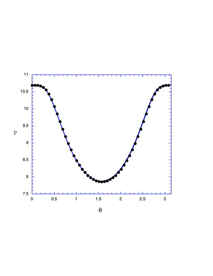
FIG. 1.: The analytic values (line) and numerical values (dots) of $P$ are plotted vs. $\theta$ at $\tau=10$.

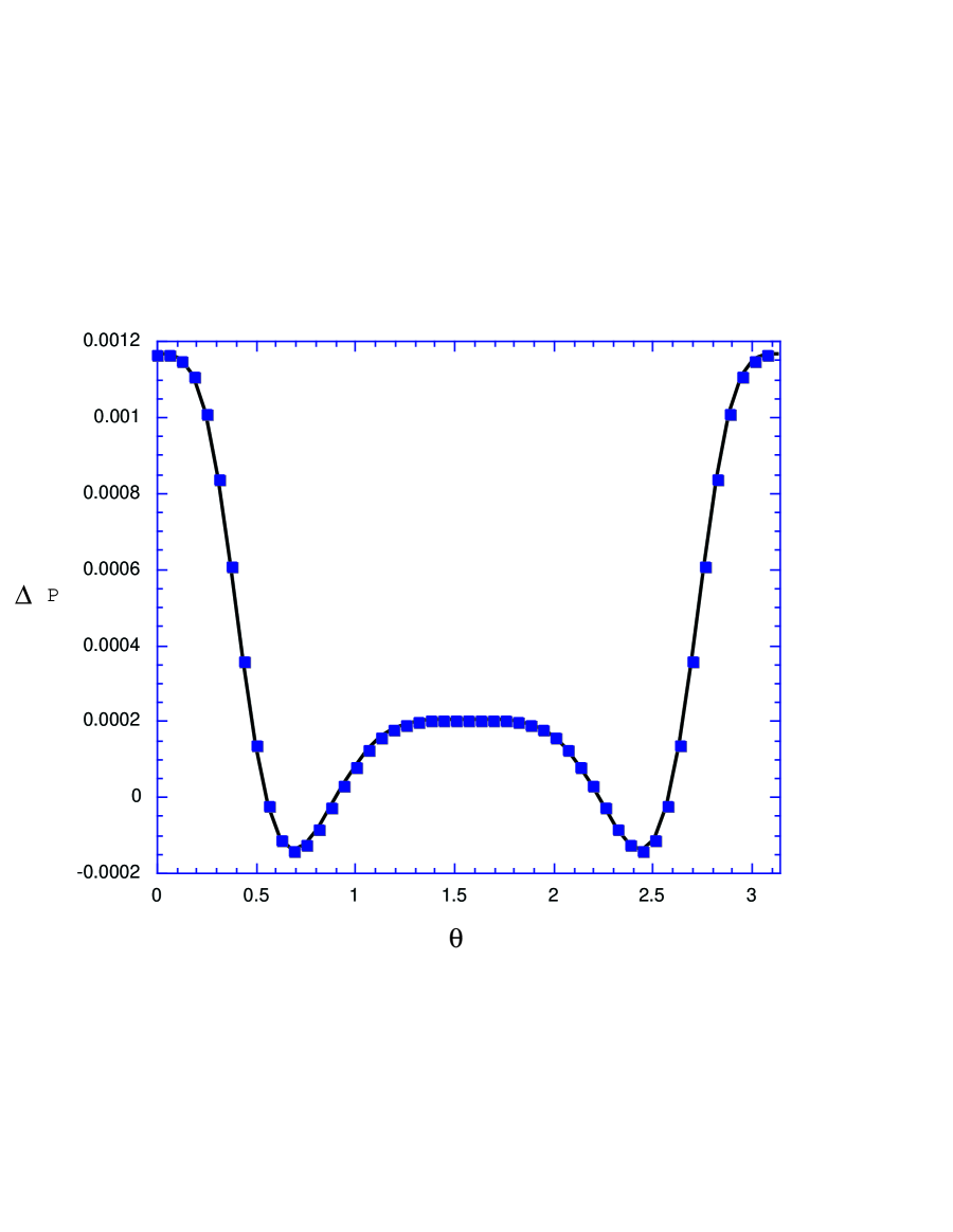
FIG. 2.: The differences between analytic and numerical values for $P$ are compared for two different resolutions. The line is $\Delta P$ for 502 grid points and the squares are 4 times $\Delta P$ for 1002 grid points. The fact that these curves agree shows second order convergence

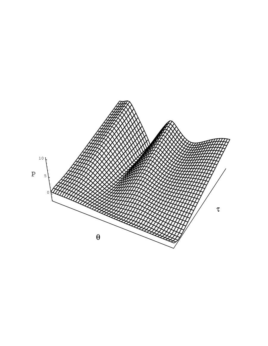
FIG. 3.: The evolution of $P$ for initial data with ${v_{0}}=2$.

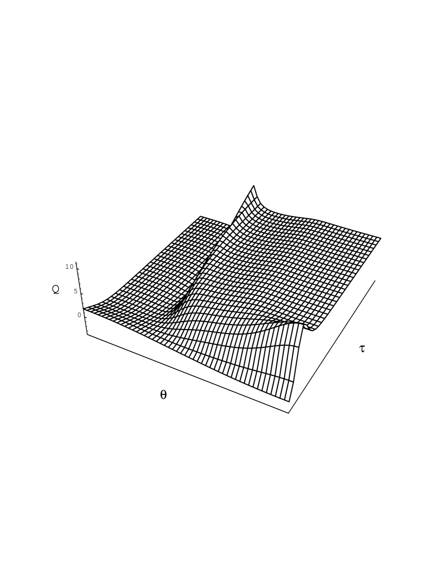
FIG. 4.: The evolution of $Q$ for initial data with ${v_{0}}=2$.

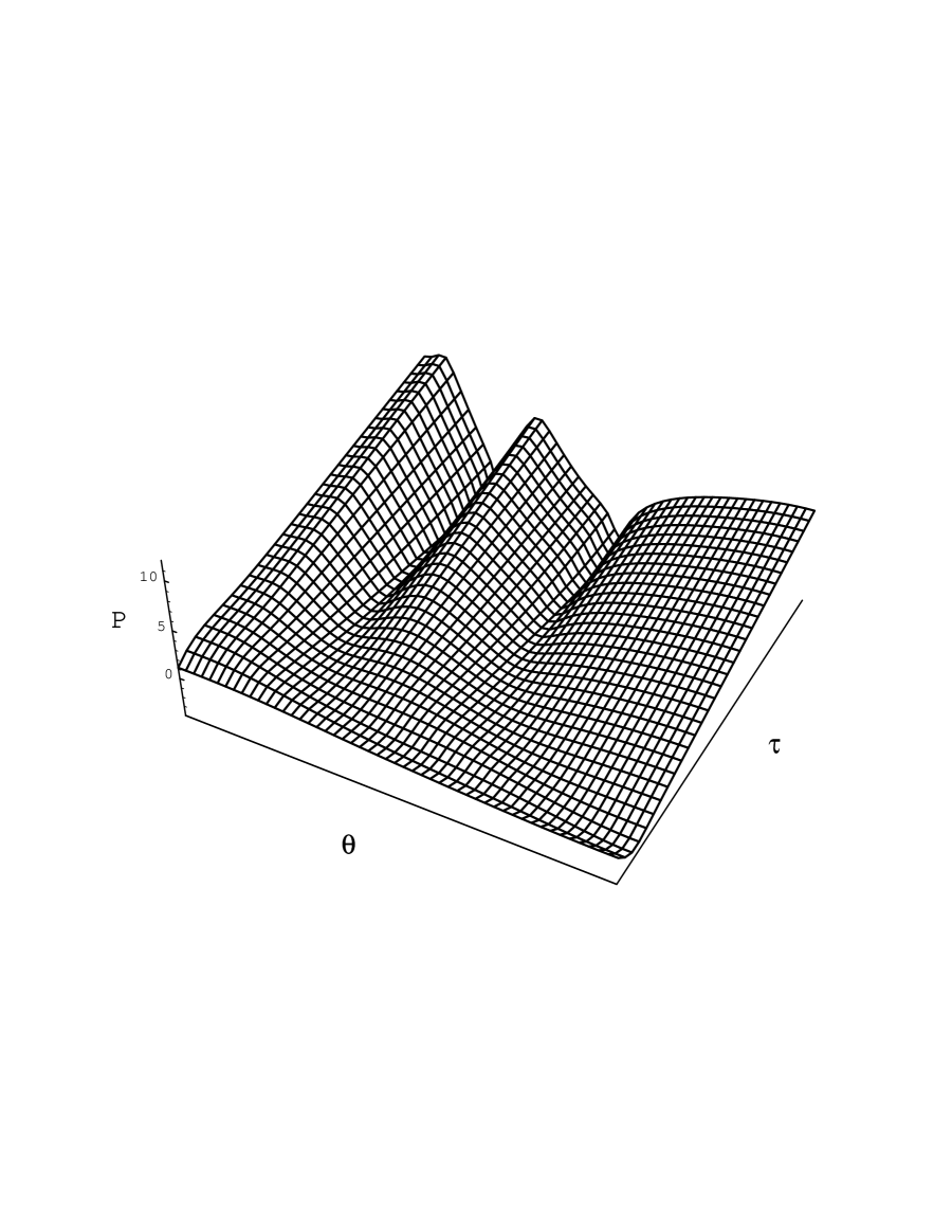
FIG. 5.: The evolution of $P$ for initial data with ${v_{0}}=4$.

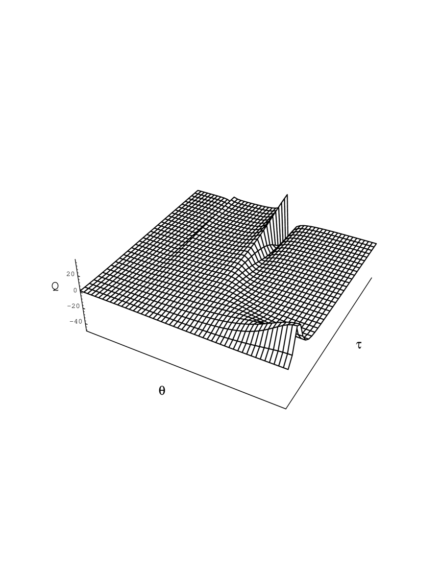
FIG. 6.: The evolution of $Q$ for initial data with ${v_{0}}=4$.

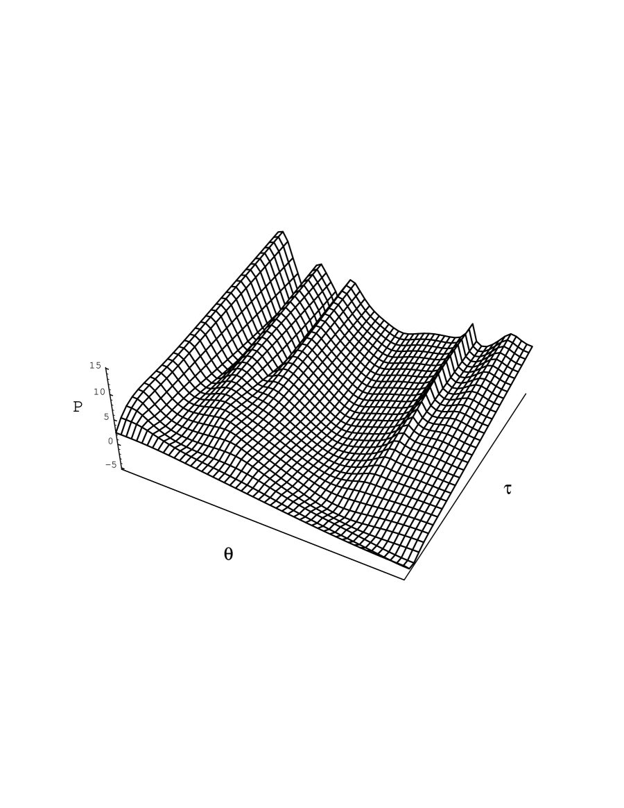
FIG. 7.: The evolution of $P$ for initial data with ${v_{0}}=8$.

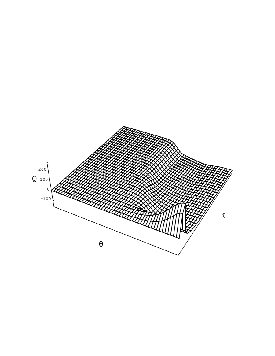
FIG. 8.: The evolution of $Q$ for initial data with ${v_{0}}=8$.

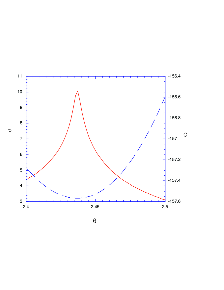
FIG. 9.: a spiky feature in $P$ (solid line) occurs where $Q$ (dashed line) has an extremum. Here, ${v_{0}}=8,\,\tau=10$ and the simulation is run with 2002 spatial grid points.

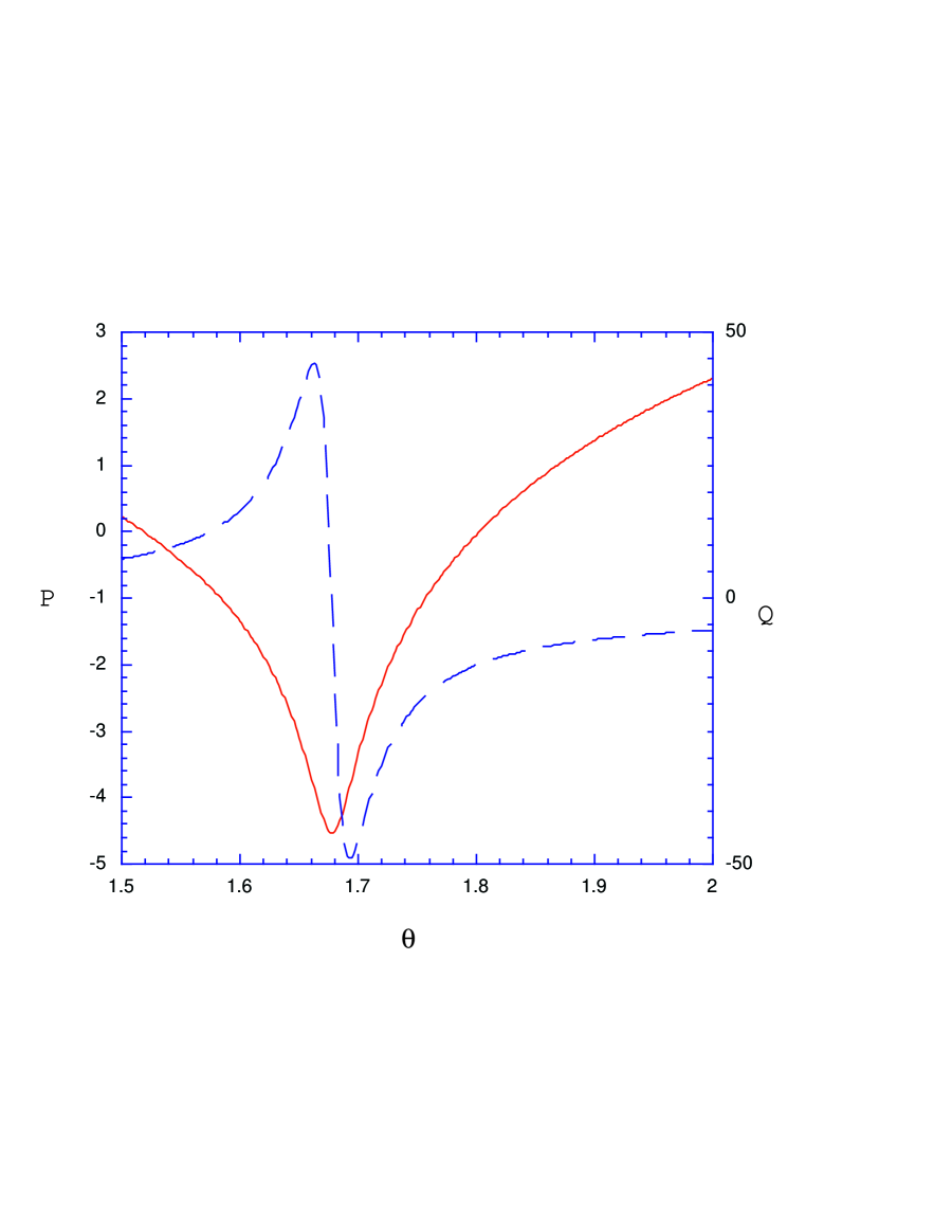
FIG. 10.: a sharp feature in $Q$ (dashed line) occurs at a downward spike in $P$ (solid line). Here, ${v_{0}}=4,\,\tau=10$ and the simulation is run with 2002 spatial grid points.

REFERENCES

- [1] B.K. Berger and V. Moncrief, Phys. Rev. D48, 4676 (1993)
- [2] B.K. Berger, D. Garfinkle and V. Swamy, Gen. Rel. Grav. 27, 511 (1995)
- [3] B.K. Berger and D. Garfinkle, Phys. Rev. D57, 4767 (1998)
- [4] M. Weaver, J. Isenberg and B.K. Berger, Phys. Rev. Lett. 80, 2984 (1998)
- [5] B.K. Berger and V. Moncrief, Phys. Rev. D57, 7235 (1998)
- [6] B.K. Berger and V. Moncrief, Phys. Rev. D58, 064023 (1998)
- [7] B.K. Berger, D. Garfinkle, J. Isenberg, V. Moncrief and M. Weaver, Mod. Phys. Lett. A13, 1565 (1998)
- [8] S.D. Hern and J.M. Stewart, Class. Quantum Grav. 15, 1581 (1998)
- [9] For a precise definition of AVTD as well as a proof that polarized Gowdy spacetimes are AVTD see J. Iseberg and V. Moncrief, Ann. Phys. (N.Y.) 199, 84 (1990)
- [10] R.H. Gowdy, Phys. Rev. Lett. 27, 826 (1971)
- [11] R.H. Gowdy, Ann. Phys. 83, 203 (1974)
- [12] O. Obregon and M.P. Ryan, gr-qc/9810068