Perturbative evolution of conformally flat initial data for a single boosted black hole

Abstract

The conformally flat families of initial data typically used in numerical relativity to represent boosted black holes are not those of a boosted slice of the Schwarzschild spacetime. If such data are used for each black hole in a collision, the emitted radiation will be partially due to the “relaxation” of the individual holes to “boosted Schwarzschild” form. We attempt to compute this radiation by treating the geometry for a single boosted conformally flat hole as a perturbation of a Schwarzschild black hole, which requires the use of second order perturbation theory. In this we attempt to mimic a previous calculation we did for the conformally flat initial data for spinning holes. We find that the boosted black hole case presents additional subtleties, and although one can evolve perturbatively and compute radiated energies, it is much less clear than in the spinning case how useful for the study of collisions are the radiation estimates for the “spurious energy” in each hole. In addition to this we draw some lessons on which frame of reference appears as more favorable for computing black hole collisions in the close limit approximation.

I Introduction

There is significant interest in obtaining waveforms for the gravitational radiation produced in the collision of black holes. Progress is being made on this problem both using supercomputers [1] and perturbative calculations [2]. One of the open issues is what families of initial data are appropriate to represent the collision of two black holes, especially when the latter are not far away from each other. The state of the art of numerical simulations suggests that for some time we may not be able to start simulations with the black holes at a sufficiently large separation, such that one can assume a simple linear superposition will work. This leaves open the issue of how much “spurious radiation” is one introducing in the various proposals for superpositions in the non-linear regime. Bowen and York [3] (and with a different set of boundary conditions more recently Brandt and Brügmann [4]) studied the problem of giving initial data for boosted and spinning holes in such a way that a superposition is possible. They assume the spatial metric is conformally flat and as a consequence one can superpose the extrinsic curvatures for the two holes and still solve the momentum constraint. One then proceeds to find a conformally flat spatial metric for the superposed holes by solving a nonlinear elliptic partial differential equation. The procedure achieves superposition at the price of assuming conformal flatness of the three metrics, which is not generically possible, and more importantly, is not possible in situations of interest. For instance a single spinning black hole, described by the Kerr solution, is not known to admit conformally flat spatial slices [3].

A similar situation develops for the case of a single boosted black hole. The initial data constructed by Bowen and York or Brandt and Brügmann do not correspond to those one would find on a boosted slice of the Schwarzschild spacetime. In this paper we will refer to these families as “conformal boosted black hole” Therefore if one evolves these families of data one should find that the black hole “settles down” to a Schwarzschild form through the emission of gravitational radiation. The original purpose of this paper was to study the emitted radiation by treating the conformal boosted hole as a perturbation of a Schwarzschild black hole. In a previous paper we had carried out a similar discussion for the case of a single spinning conformally flat hole [5]. We will see that the boosted case is much more subtle than anticipated. We will be able to evolve the spacetime, but questions will remain about the usefulness of the results obtained, at least for the original purpose of gaining insight into the spurious radiation content of data for black hole collisions for interesting ranges of parameter values.

The organization of this paper is as follows. In the next section we will discuss perturbations of a boosted black hole. We recall that the $\ell=1$ even modes are pure gauge and therefore all the physics of interest takes place in the $\ell=2$ modes, which can be treated easily up to second order in perturbation theory. In section III we will discuss the perturbative evolution and the amount of radiation produced. We end with a discussion of the results and their implication for the choice of frame of reference one uses in perturbative evolutions of black hole collisions with linear momentum.

II Conformal boosted black hole as a perturbation of Schwarzschild

A Initial data in the conformal approach

The families of initial data that we will consider in this paper are obtained via the “conformal approach” to the initial value problem in general relativity. In it, one assumes the metric to be conformally flat $g_{ab}=\phi^{4}\delta_{ab}$ and defines the conformal extrinsic curvature $\widehat{K}_{ab}=\phi^{2}K_{ab}$. In terms of these variables the initial value constraint equations (assuming maximal slicing ${\rm Tr}K=0$) read,

$$\nabla_{a}\widehat{K}^{ab} = 0$$ (1)

$$\nabla^{2}\phi = -{1\over 8}{\widehat{K}^{ab}\widehat{K}_{ab}\over\phi^{7}}$$ (2)

where all the derivatives are with respect to flat space.

One can construct [3] solutions to the first set of equations (momentum constraint) for a single black hole centered at $R=0$, with linear momentum $P_{a}$,

$$\widehat{K}_{ab}={3\over 2R^{2}}\left[2P_{(a}n_{b)}-(\delta_{ab}-n_{a}n_{b})P^{c}n_{c}\right]\ .$$ (3)

where $R$ is a spherical radial coordinate and $n_{a}$ a radial unit vector, and both are defined in the fiducial flat space that one obtains setting the conformal factor to unity.

Without loss of generality we may assume that $P_{a}$ points along the positive z-axis, and has magnitude $P$. If we write $\widehat{K}_{ab}$ in spherical coordinates, the only non vanishing components are

$$\widehat{K}_{RR} = {3P\over R^{2}}\cos(\theta)$$ (4)

$$\widehat{K}_{R\theta} = -{3P\over 2R}\sin(\theta)=\widehat{K}_{\theta R}$$ (5)

$$\widehat{K}_{\theta\theta} = -{3P\over 2}\cos(\theta)$$ (6)

$$\widehat{K}_{\phi\phi} = \sin(\theta)^{2}\widehat{K}_{\theta\theta}$$ (7)

If we write the extrinsic curvature in terms of tensor spherical harmonics [6], we see that it consists of a pure $\ell=1$ even term. This is reasonable, since the presence of momentum in an initial slice configuration is determined by the presence of a “dipole” term asymptotically, that makes the ADM integral

$$P_{i}={1\over 8\pi}\int_{\infty}K_{ij}d^{2}S_{j}$$ (8)

nonvanishing.

From (7), we have,

$$\widehat{K}_{ab}\widehat{K}^{ab}={9P^{2}\over 2R^{4}}\left(1+2\cos^{2}\theta\right)$$ (9)

We now need to solve (2), and this involves imposing boundary conditions on $\phi$. One possibility is that given by Bowen and York [3]. In this case one chooses a certain constant $a$, solves (2) for $R\geq a$, and imposes

$${\partial\phi\over\partial R}+{1\over 2R}\phi=0\;\;\mbox{for}\;\;R=a,$$ (10)

and

$$\phi>0\;\;,\;\;\lim_{R\rightarrow\infty}\phi=1.$$ (11)

It should be clear that, in addition to the choices we originally made, there are other choices made in constructing the solutions. As suggested by Bowen and York, a possibility that can be considered appealing, especially when one has multiple black holes, consists in requesting that both the conformal factor and the extrinsic curvature be symmetrized through the throats of the holes. This was implemented explicitly by Cook [8] in his numerical work on constructing solutions for the conformal factor for multiple black holes. The symmetrization procedure yields non-trivial results even for a single black hole as we are considering here [10]. We have chosen, for simplicity, not to symmetrize the extrinsic curvature. However, the boundary condition (10) automatically ensures that the conformal factor be symmetric (provided one chose a symmetric extrinsic curvature). One could perform other choices and the problem is simple enough that —at the level of approximation we are working— it can always be solved. Perhaps the choice we make here is not the most aesthetically appealing to some readers, but experience has shown that symmetrizing or not symmetrizing does not change significantly the amount of radiated energy in head-on black hole collisions [11]. Therefore our choice should not crucially influence the central conclusions we are attempting to obtain about the conformally flat black hole solutions. It should be noticed that with our choice of non-symmetric extrinsic curvature, condition (10) implies that the surface where it is applied is an extremal surface (not necessarily minimal).

Even for the simple form of (9), in general we cannot solve (2) exactly, and one has to resort to numerical methods. In the present analysis, however, we will be interested in solutions for “small” $P$. Since for $P=0$ the solution is

$$\phi^{(0)}=1+{a\over R}$$ (12)

we may solve (2) iteratively replacing

$$\phi=\phi^{(0)}(R)+P^{2}\phi^{(2)}(R,\theta)+P^{4}\phi^{(4)}(R,\theta)+\cdots$$ (13)

in (2), and imposing

$${\partial\phi^{(i)}\over\partial R}+{1\over 2R}\phi^{(i)}=0\;\;\mbox{for}\;\;R=a,\;\;\;\;\;\lim_{R\rightarrow\infty}\phi^{(i)}=0.\;\;\mbox{for}\;\;i\neq 0,$$ (14)

The form of (9) further suggests that we expand $\phi^{(i)}$ in Legendre polynomials $P_{\ell}(\cos\theta)$, so that $\phi^{(2)}$ may be written as

$$\phi=\phi^{(0)}(R)+P^{2}\left[\phi^{(2)}_{0}(R)P_{0}(\cos\theta)+\phi^{(2)}_{2}(R)P_{2}(\cos\theta)\right]+{\cal{O}}(P^{4}).$$ (15)

Solving for the coefficients taking into account the boundary condition (10) we get,

$$\phi^{(2)}_{0}(R) = {(R+a)^{5}-R^{5}\over 32a^{2}(R+a)^{5}}+{13\over 512aR}$$ (16)

$$\phi^{(2)}_{2}(R) = {75R^{6}+291aR^{5}-650a^{2}R^{4}-3400a^{3}R^{3}-4800a^{4}R^{2}-2925a^{5}R-669a^{6}\over 400R^{3}(R+a)^{5}}$$ (18)

$$+{21a\over 20R^{3}}[\ln(2a)-\ln(R+a)]+{121a\over 128R^{3}}$$

Notice that $\phi^{(2)}_{2}(R)$ falls off only as $R^{-2}$ for large $R$.

For completeness, we also present the solution one obtains if one chooses the “puncture” boundary condition considered by Brandt and Brügmann [4] recently,

$$\phi^{(2)}_{0}(R) = {\frac{{M}^{4}+10\,{M}^{3}R+40\,{M}^{2}{R}^{2}+80\,M{R}^{3}+80\,{R}^{4}}{8\,M\left(2\,R+M\right)^{5}}}$$ (19)

$$\phi^{(2)}_{2}(R) = {\frac{120\,{R}^{5}+768\,{R}^{4}M+1078\,{R}^{3}{M}^{2}+658\,{R}^{2}{M}^{3}+189\,R{M}^{4}+21\,{M}^{5}}{20\,{R}^{2}\left(2\,R+M\right)^{5}}}$$ (21)

$$-21{\frac{\left(\ln(2\,R+M)-\ln(M)\right)M}{40\,{R}^{3}}}$$

but we will only consider the solution (18) in the rest of this paper.

To obtain an initial data set appropriate for a perturbative evolution we proceed in two steps. If, in an ADM type decomposition, we choose our shift functions $N_{i}=0$, we have,

$$ds^{2} = g_{ij}dx^{i}dx^{j}-N^{2}(dt)^{2}$$ (22)

$${\partial g_{ij}\over\partial t} = -2NK_{ij}$$ (23)

where, for the initial slice, that we may take as $t=0$, the 3-metric $g_{ij}$ and extrinsic curvature $K_{ij}$ are given by the above construction. We next change the conformal spherical radial coordinates $R$, to a “Schwarzschild” radial coordinates $r$, with $R=(\sqrt{r}+\sqrt{r-2M})^{2}/4$, and choose $N=\sqrt{1-2M/r}$, so that we recover the Schwarzschild metric for $P=0$. The perturbation treatment refers to this last form of the metric. It should be noticed that the extrinsic curvature to consider in (22) should be the physical one obtained dividing by the conformal factor squared the conformal extrinsic curvature (7).

Carrying out all these steps we find that the initial data has the following multipolar components: to zeroth order in the momentum, we only have $\ell=0$ components; to first order in the linear momentum, only $\ell=1$ contributions; to order ${\cal O}(P^{2})$, we have $\ell=0,2$ contributions. All contributions are even-parity.

B Multipolar decomposition of the initial data : the $\ell=1$ contributions

The contribution to the three-metric of zeroth order in $P$ is just the Schwarzschild solution. The first apparently non-trivial contribution is given at ${\cal O}(P^{1})$ and corresponds as we discussed in the previous subsection to an $\ell=1$ multipole. Let us analyze the $\ell=1$ perturbations of a spherically symmetric spacetime. In order to do this we use the traditional Regge–Wheeler [6] decomposition. One starts with a background metric written as,

$$g^{(0)}_{\mu\nu}dx^{\mu}dx^{\nu}=-(1-2M/r)\;dt^{2}+(1-2M/r)^{-1}dr^{2}+r^{2}d\theta^{2}+r^{2}\sin^{2}\theta d\varphi^{2}.$$ (24)

For axisymmetric perturbations, the general $\ell=1$ even parity terms take the form [6]

$$h^{(1)}_{tt} = (1-2M/r)H_{0}(t,r)\cos\theta$$ (25)

$$h^{(1)}_{tr} = H_{1}(t,r)\cos\theta$$ (26)

$$h^{(1)}_{rr} = (1-2M/r)^{-1}H_{2}(t,r)\cos\theta$$ (27)

$$h^{(1)}_{t\theta} = -h_{0}(t,r)\sin\theta$$ (28)

$$h^{(1)}_{r\theta} = -h_{1}(t,r)\sin\theta$$ (29)

$$h^{(1)}_{\theta\theta} = r^{2}K(t,r)\cos\theta$$ (30)

$$h^{(1)}_{\phi\phi} = r^{2}\sin^{2}\theta K(t,r)\cos\theta$$ (31)

The first order metric perturbation coefficients are not uniquely defined, but may be changed by “gauge transformations” of the form [6]

$$\widetilde{h}^{(1)}_{\mu\nu}=h^{(1)}_{\mu\nu}-g_{\mu\nu},_{\rho}\xi_{(1)}^{\rho}-g_{\mu\rho}\xi_{(1)}^{\rho},_{\nu}-g_{\rho\nu}\xi_{(1)}^{\rho},_{\mu}$$ (32)

where the gauge 4-vector $\xi_{(1)}^{\mu}$ is arbitrary, except for the requirement of axisymmetry.

In particular, the $\ell=1$ even parity coefficients transform as

$$\widetilde{H}_{0}(t,r) = H_{0}(t,r)+2{\partial{\cal{M}}_{0}(t,r)\over\partial t}+{2M\over r(r-2M)}{\cal{M}}_{1}(t,r)$$ (33)

$$\widetilde{H}_{1}(t,r) = H_{1}(t,r)+{r-2M\over r}{\partial{\cal{M}}_{0}(t,r)\over\partial r}-{r\over r-2M}{\partial{\cal{M}}_{1}(t,r)\over\partial t}$$ (34)

$$\widetilde{H}_{2}(t,r) = H_{2}(t,r)+{2M\over r(r-2M)}{\cal{M}}_{1}(t,r)-2{\partial{\cal{M}}_{1}(t,r)\over\partial r}$$ (35)

$$\widetilde{h}_{0}(t,r) = h_{0}(t,r)+{r-2M\over r}{\cal{M}}_{0}(t,r)-r^{2}{\partial{\cal{M}}_{2}(t,r)\over\partial t}$$ (36)

$$\widetilde{h}_{1}(t,r) = h_{1}(t,r)-{r\over r-2M}{\cal{M}}_{1}(t,r)-r^{2}{\partial{\cal{M}}_{2}(t,r)\over\partial r}$$ (37)

$$\widetilde{K}(t,r) = K(t,r)-{2\over r}{\cal{M}}_{1}(t,r)+2{\cal{M}}_{2}(t,r)$$ (38)

where the functions ${\cal{M}}_{i}$ are arbitrary.

One can use this gauge freedom to go to a restricted gauge in which $h_{0}=h_{1}=K=0$. This gauge is not completely fixed. One still can perform gauge transformations of the form,

$${\cal{M}}_{0}={r^{3}\over r-2M}{\partial{\cal{M}}_{2}\over\partial t}\;\;\;,\;\;\;{\cal{M}}_{1}=r{\cal{M}}_{2}\;\;\;,\;\;\;{\cal{M}}_{2}={f(t)\over r-2M}$$ (39)

where $f(t)$ is arbitrary.

An interesting result, is that in this gauge it is straightforward to find the general solution of the linearized Einstein equations for $\ell=1$ even parity perturbations. The result is,

$$H_{1} = -{r\over(r-2M)^{2}}{dF_{1}\over dt}$$ (40)

$$H_{0} = {1\over 3(r-2M)^{2}}F_{1}+{r^{3}\over 3M(r-2M)^{2}}{d^{2}F_{1}\over dt^{2}}$$ (41)

$$H_{2} = {1\over(r-2M)^{2}}F_{1}(t),$$ (42)

where $F_{1}(t)$ is an arbitrary function. Remarkably, one can show that this solution is pure gauge. Choosing $f(t)=-F_{1}(t)/(6M)$ in (39) leads to vanishing gauge transformed quantities.

We therefore see that the $\ell=1$ perturbations are pure gauge. This result was first noticed by Zerilli [12]. This was to be expected in physical grounds since one could always imagine setting coordinates boosted in such a way that the black hole would not move. It has the further implication that we can compute the radiated energy by computing the $\ell=2$ perturbations in a gauge in which the $\ell=1$ perturbations vanish, and studying their evolution.

C Multipolar decomposition of the initial data : the $\ell=2$ contributions

The relevant $\ell=2$ perturbations are of second order in our perturbation parameter, $P$. In principle, when one works out second order perturbations of a given metric, the evolution equations one gets have the general form of a linear operator (similar to the one that acts in first order giving rise to the Zerilli equation) acting on second order quantities, equal to a quadratic “source” term formed with the first order perturbations [13]. The source term is complicated and is delicate to handle numerically when evolving the perturbations. A place where this was explicitly done was for instance in the evolution of boosted black hole collisions to second order [11]. The calculations are lengthy and complicated. Fortunately, in our case one can proceed in a different way. We have just shown that there is a gauge in which the first order perturbations (the $\ell=1$ ones) vanish. Therefore in that gauge one can write a second order Zerilli equation that is source-free. Moreover, the linear portion of the second order perturbative equation is exactly the same as the first order perturbative equation (the Zerilli equation), and this equation can be written in terms of quantities that are gauge invariant. We notice, however, that eliminating the first order $\ell=1$ terms through a first order gauge transformation introduces second-order changes in the metric that are not a pure second order gauge transformation, and must be taken into account. One must then be careful in making sure that the initial data for the $\ell=2$ perturbations used in the Zerilli equation corresponds precisely to that gauge. In other words, we need to carry out a first order gauge transformation on the initial data that provides a new initial data corresponding to a gauge where the $\ell=1$ perturbations vanish. Since all perturbations satisfy equations that are second order in time, this requires that the $\ell=1$ terms of the metric, and their first time derivative vanish on the initial slice. If we consider (33), this requires that the gauge vector components ${\cal{M}}_{i}$ are such that both the left hand sides in (33), and their first time derivatives, vanish when evaluated at $t=0$. This, in principle requires only the knowledge of the metric functions on the right hand side of (33), and their first time derivative, at the fiducial time $t=0$. It turns out, however, that we also need second order time derivatives,

to implement the second order gauge transformation required to obtain the $\ell=2$ initial data. These second order time derivatives may be straighforwardly evaluated from the corresponding Einstein equations for the $\ell=1$ perturbations.

For the particular case in question, the $\ell=1$ initial data (and first time derivative) is determined by (4), and one can use this information to construct the space-time solution of the Einstein equations produced by the initial data as a Taylor expansion in $t$, up to the appropriate order. One gets, using the usual Regge-Wheeler notation [6] the following expansions for the $\ell=1$ components of the metric,

$$H_{2} = -{3\over 2}{(\sqrt{r}+\sqrt{r-2M})^{2}\sqrt{r-2M}\over r^{7/2}}Pt+O(t^{3})$$ (43)

$$K = {3\over 4}{(\sqrt{r}+\sqrt{r-2M})^{2}\sqrt{r-2M}\over r^{7/2}}Pt+O(t^{3})$$ (44)

$$h_{1} = -{3\over 4}{(\sqrt{r}+\sqrt{r-2M})^{2}\over r^{2}}Pt+O(t^{3})$$ (45)

all the other components being $O(t^{3})$.

The components of the gauge vector generating the first order gauge transformation that makes the initial $\ell=1$ data purely $O(t^{3})$ are,

$$\xi_{t} = {\cal{M}}_{0}\cos\theta$$ (46)

$$\xi_{r} = {\cal{M}}_{1}\cos\theta$$ (47)

$$\xi_{\theta} = -{\cal{M}}_{2}\sin\theta$$ (48)

$$\xi_{t} = 0,$$ (49)

where,

$${\cal{M}}_{0} = -{\frac{P\left(-3\,\sqrt{r-2\,M}rM-5\,{r}^{3/2}M+2\,{M}^{2}\sqrt{r}+2\,{r}^{5/2}+2\,\sqrt{r-2\,M}{r}^{2}\right)}{4\,\sqrt{r}M\left(r-2\,M\right)}}$$ (50)

$${\cal{M}}_{1} = -{\frac{P\left(-6\,\sqrt{r-2\,M}rM+2\,{r}^{5/2}-8\,{r}^{3/2}M+8\,{M}^{2}\sqrt{r}+3\,\sqrt{r-2\,M}{M}^{2}+2\,\sqrt{r-2\,M}{r}^{2}\right)t}{4\,{r}^{5/2}M}}$$ (51)

$${\cal{M}}_{2} = -{\frac{P\left(-3\,\sqrt{r-2\,M}rM-5\,{r}^{3/2}M+2\,{M}^{2}\sqrt{r}+2\,{r}^{5/2}+2\,\sqrt{r-2\,M}{r}^{2}\right)t}{4\,{r}^{7/2}M}}.$$ (52)

Performing a first order gauge transformation with this generator, one eliminates the first order $\ell=1$ component of the metric. Therefore the leading terms in the initial data become second order. The latter have two contributions, both of $\ell=2$ multipolar order. One contribution simply comes from the expansion to second order of the initial data generated via the conformal approach. The other contribution comes from the fact that the first order gauge transformation we just performed has second order pieces of the form,

$$\widetilde{h}^{(2)}_{\mu\nu} = h^{(2)}_{\mu\nu}$$ (55)

$$-\widetilde{h}^{(1)}_{\mu\nu},_{\rho}\xi_{(1)}^{\rho}-\widetilde{h}^{(1)}_{\mu\rho}\xi_{(1)}^{\rho},_{\nu}-\widetilde{h}^{(1)}_{\rho\nu}\xi_{(1)}^{\rho},_{\mu}$$

$$-{1\over 2}g_{\mu\nu},_{\sigma},_{\lambda}\xi_{(1)}^{\sigma}\xi_{(1)}^{\lambda}-g_{\mu\lambda},_{\sigma}\xi_{(1)}^{\sigma}\xi_{(1)}^{\lambda},_{\nu}-g_{\lambda\nu},_{\sigma}\xi_{(1)}^{\sigma}\xi_{(1)}^{\lambda},_{\mu}-g_{\sigma\lambda}\xi_{(1)}^{\sigma},_{\mu}\xi_{(1)}^{\lambda},_{\nu}$$

The contribution to the second order Zerilli function coming from the nonlinear terms in the gauge transformation can be found after a straightforward but tedious calculation. The relevant contributions to the second order $\ell=2$ metric at $t=0$, are,

$${}^{(2)}K = {2\over 3}{P^{2}R^{2}\over M^{2}r^{3}}$$ (56)

$${}^{(2)}H_{2} = {2\over 3}{P^{2}R^{2}(R-M)^{2}\over M^{2}r^{3}(r-2M)}$$ (57)

$${}^{(2)}h_{1} = {1\over 3}{P^{2}R^{5/2}(R-M)\over M^{2}r^{3/2}(r-2M)}$$ (58)

$${}^{(2)}G = {1\over 3}{P^{2}R^{2}\over M^{2}r^{3}}$$ (59)

where $R=(\sqrt{r}+\sqrt{r-2M})^{2}/4$.

Another contribution to this initial data comes from the second order corrections to the conformal factor, calculated above. These contributions to the second order $\ell=2$ metric all vanish, except for,

$${}^{(2)}H_{2} = 4P^{2}\left(1+{M\over 2R}\right)^{3}\phi^{(2)}_{2}(R){R^{2}\over r^{2}}$$ (60)

$${}^{(2)}K = {}^{(2)}H_{2},$$ (61)

and all first order time derivatives vanish.

The Zerilli function in an arbitrary gauge is given by [14],

$$\psi(t,r) = \frac{r(r-2M)}{3(2r+3M)}\left[{\ }^{(2)}{H}_{2}-r\frac{\partial{\ }^{(2)}{K}}{\partial r}-\frac{r-3M}{r-2M}{\ }^{(2)}{K}\right]$$ (63)

$$+{r^{2}\over 2r+3M}\left[{\ }^{(2)}{K}+(r-2M)\left(\frac{\partial{\ }^{(2)}{G}}{\partial r}-{2\over r^{2}}{\ }^{(2)}{h}_{1}\right)\right].$$

Substituting the above components yields the following initial data for the Zerilli function,

$$\psi(t=0,r)=P^{2}\left[{(3M+8R)R^{2}\over 6M^{2}r(2r+3M)}+{4r(2M+3R)\over 3(2r+3M)}\phi^{(2)}_{2}(R)-{(4r-8M)R^{1/2}r^{3/2}\over 3(2r+3M)}\left({\partial\phi^{(2)}_{2}(R)\over\partial r}\right)\right]$$ (64)

$$\left.{\partial\psi(t,r)\over\partial t}\right|_{t=0}=0.$$ (65)

For the conformal factor we computed in (18), this results in,

$$\psi(t=0,r) = {P^{2}R^{6}\over M(M+2R)^{4}(M^{2}+10MR+4R^{2})}\left({128\over 3}+56{M\over R}+{6113\over 25}{M^{2}\over R^{2}}+{32607\over 100}{M^{3}\over R^{3}}\right.$$ (68)

$$\left.+{3882\over 25}{M^{4}\over R^{4}}-{235\over 16}{M^{5}\over R^{5}}-{691\over 16}{M^{6}\over R^{6}}-{26679\over 1600}{M^{7}\over R^{7}}-{2047\over 800}{M^{8}\over R^{8}}-{2327\over 19200}{M^{9}\over R^{9}}\right)$$

$$+{7P^{2}M(M+12R)(M+2R)^{2}(\ln(2M)-\ln(M+2R))\over 40R^{3}(M^{2}+10MR+4R^{2})}.$$

D Physical validity of the perturbative treatment

Inspecting the initial data for the Zerilli function one finds that it behaves in a non-conventional way. Here is where we note significant differences with the case of single spinning holes [5].

The first unusual thing one notices is that the initial data goes asymptotically to a constant value for $R\rightarrow\infty$. This is different from the data for the “close limit” of two black holes (momentarily stationary or boosted) where the Zerilli function goes to zero at infinity. The root of this problem can be traced down to the falloff conditions of the extrinsic curvature. In all other cases in which the “close limit” approximation has been applied, the extrinsic curvature falls off as $1/r^{3}$ at infinity. For the case in this paper, it decreases as $1/r^{2}$ (otherwise the momentum would vanish). This, in particular, leads to falloff conditions in the gauge vectors we use to eliminate the $\ell=1$ even pieces of the extrinsic curvature. In turn, the falloff condition of the gauge vectors influences, via the quadratic terms in the second order gauge transformation, the behavior of the Zerilli function we obtain at the end of the process.

Does the appearance of a Zerilli function that does not vanish at infinity indicate something problematic in itself? We do not seem to see any difficulty in evolving the problem in this case. Our evolution code evolves a “slab” region consistent of the initial data and its domain of dependence, therefore we do not need to specify any boundary conditions. If one observes the behavior of the Zerilli function as a function of time for a fixed (finite) value of the radius, it starts having a constant value followed by a quasinormal ringing and a power law tail decrease towards zero. That is, the constant behavior at infinity translates itself in a certain behavior at the beginning of the waveform, it does not leave any visible effect after the ringdown and power law tail behavior. The radiated energy and all observable quantities at infinity (even to second order in perturbation theory, see section III.B of [9]) are not determined by the Zerilli function itself but by its time derivative, for which the initial data indeed goes to zero for large values of the radius, and therefore no problem in the evaluation of physical quantities is present.

Another aspect that could cause concern is the nature of the gauge transformation considered. The gauge transformation is well behaved in any finite value of $r_{*}$ (that is, any point of the exterior of the black hole excluding the horizon and spatial infinity). Since in order to compute the radiated energies and waveforms we will never need information from either the horizon nor infinity, the gauge transformation is well defined in all relevant points for our calculation.

III Results and conclusions

We have numerically evolved the Zerilli equation with the initial data presented above and computed the energy and waveforms for the “relaxation” of a single boosted Bowen–York hole to a boosted Schwarzschild black hole. The results for the energy can be summarized by a simple formula which, to leading order in $P$ reads,

$$\left({E_{\rm radiated}\over M_{ADM}}\right)=4.1\times 10^{-2}\left({P\over M_{ADM}}\right)^{4}$$ (69)

where the prefactor was computed numerically .

Figure 1 shows the radiated energy as a function of the momentum. We see that for values of the momentum close to $P/M_{ADM}\sim 0.4$ the total radiated energy by the “relaxation” of a single boosted Bowen–York black hole to a Schwarzschild black hole is similar to the total radiated energy in a close limit collision of Bowen–York black holes [11] and figure 2. One could therefore be tempted to say that for values of $P/M_{ADM}>0.4$ one should stop using these families of initial data. A puzzling element is that we have already evolved these families of initial data in collision situations and compared with actual non-linear integrations of the Einstein equations [15, 11] and we know that these families of initial data radiate less in collisions than the values we are predicting here for each individual hole, at least for close separations. The results for these collisions are recollected in figure 2.

What is going on? One has to keep these results in perspective, since it is easy to get carried away and believe that perturbation theory should work way beyond where it was meant to do so. In the calculation of the present paper we find that the radiated energy goes as $P^{4}$. This is good, since our perturbative parameter is $P$ and therefore this means that the corrections are small. In the case of colliding black holes the radiated energies contain terms that go as (see reference [11]) $L^{4}$, $P^{2}L^{2}$ and $PL^{3}$, where $L$ is the separation of the black hole centers in the conformally related flat space. If one simply increases the value of $P$ keeping $L$ constant, it is obvious that the contribution we consider in this paper will quickly dominate. However, one is clearly pushing things beyond the realm in which these calculations were meant to be reliable. One is essentially forcing a higher order term in perturbation theory to a regime in which it is larger than the lower order terms!

Therefore the conclusion of this paper has to be read in the following way: the terms coming from the “relaxation” of a conformally flat hole to a usual boosted slice of Schwarzschild are higher order in perturbation theory than the ones one obtains in a collision. Because of this fact, they grow fast with the perturbative parameter and perturbation theory breaks down early for the estimation of the involved energy in the calculations of the current paper. The breakdown occurs earlier for a single hole than for a collision of holes (at least computed in the center-of-momentum frame).

Connected with the latter point is another interesting insight gained from the analysis of this paper. It has to do with the choice of frame used to describe collisions of black holes in perturbation theory. The situation is illustrated in figure 3. One would expect these two collisions to be physically equivalent. However, if one considers conformal black holes and expands in perturbation theory, the collision at the bottom will contain terms that behave exactly like those we discuss in the current paper, whereas the top collision does not. If we power count, for the bottom collision, the extrinsic curvature has leading terms that behave like $P$ and are $\ell=1$ and the conformal factor has terms that behave like $L^{2}$ plus terms that behave like $P^{2}$ at leading order. The energy, being quadratic in the fields, will generically contain terms that behave like $L^{4}$, $P^{2}L^{2}$ and $P^{4}$, the latter being the terms we encountered in this paper. However, the top collision contains terms $L^{4}$, $PL^{3}$ and $P^{2}L^{2}$, as discussed in reference [11] (the extrinsic curvature goes as $PL$ and the conformal factor as $L^{2}$ at leading order). Therefore if one were to consider “close” black holes and were to consider the radiated energy as a function of $P$, as we have done above, one would encounter that the perturbative predictions —at the order considered— will differ significantly as soon as the $P^{4}$ terms start to grow. The moral from this paper insofar as the choice of the origin is: perturbation theory breaks down quickly as a function of momentum for situations with net linear momentum, it is best to analyze collisions set up in the center-of-momentum frame.

As expected, given the nature of the Zerilli equation, the waveforms that one obtains from the “relaxation” just behave like quasinormal ringing. Figure 4 shows the waveform of the decay. The form is that of a typical ringdown, and it therefore takes an amount of time of the order of the light-crossing time of the black hole size to decay.

Summarizing, as in the case of spinning Bowen–York black holes, one has extra radiation present in the initial data, that grows with the value of the momentum. In evolutions of binary black hole collisions, one can either wait long enough for this energy to be “flushed away” from the system, or restrict oneself to values of the momentum that are small enough that the extra energy is small respect to the total energy produced in the collision. The latter is the only option in the case of “close limit” collisions. Another conclusion is that perturbation theory breaks down quickly as a function of the momentum of the holes for single boosted holes (and collisions of black holes not computed in the center-of-momentum frame) and therefore cannot be used to reliably estimate the “energy content” of each hole in a regime that might be of interest for the momenta and energies relevant for black hole collisions.

IV Acknowledgments

We wish to thank an anonymous referee for comments on an earlier version of this manuscript. This work was supported in part by grants of the National Science Foundation of the US INT-9512894, PHY-9423950, PHY-9800973, PHY-9407194, by funds of the University of Córdoba, the Pennsylvania State University and the Eberly Family Research Fund at Penn State. We also acknowledge support of CONICET and CONICOR (Argentina). JP also acknowledges support from the Alfred P. Sloan and John S. Guggenheim Foundations. JP was a visitor at ITP Santa Barbara during the part of the completion of this work. The authors wish to thank Richard Price and the University of Utah for hospitality. This work was supported in part by funds of the Horace Hearne Jr. Institute for Theoretical Physics.

FIG. 1.: The energy radiated in the “relaxation of a single, boosted Bowen–York black hole to a Schwarzschild black hole, as a function of the momentum. At about $P/M_{ADM}\sim 0.4$ the radiation is equivalent to the total energy radiated in a the “close limit” collision of two boosted black holes.

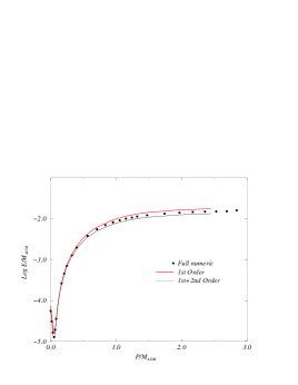
FIG. 2.: The energy radiated in the head on collision of two boosted black holes as calculated in reference 10. The collision is for two black holes separated by a Misner parameter $\mu_{0}=1.5$. Depicted are the results of first and second order perturbation theory and the full numerical results of the NCSA-Potsdam-WashU group. We see that the collisions never radiate more than $1\%$ of the ADM mass in gravitational waves.

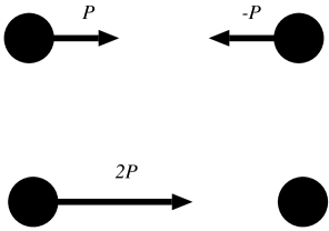
FIG. 3.: Two black hole collisions that should be physically equivalent, but that are significantly different from the point of view of the perturbative treatment involved in the “close limit approximation”.

FIG. 4.: The time derivative of the Zerilli function as a function of time. The square of this quantity is proportional to the energy flux, and therefore characterizes the “waveform” of the gravitational radiation from the decay of a Bowen–York boosted black hole into Schwarzschild.

REFERENCES

- [1] See for instance Cook et al. Phys. Rev. Lett. 80 2512 (1998), and Gómez et al. Phys. Rev. Lett. 80 3915 (1998).
- [2] J. Pullin, Prog. Theor. Phys. Suppl. 136, 107 (1999)
- [3] J. Bowen, J. York, Phys. Rev. D21, 2047 (1980).
- [4] S. Brandt, B. Brügmann, Phys. Rev. Lett. 78, 3606 (1997).
- [5] R. Gleiser, C. O. Nicasio, R. Price, J. Pullin, Phys. Rev. D57, 3401 (1998).
- [6] T. Regge, J. Wheeler, Phys. Rev. 108, 1063 (1957).
- [7] D. Brill, R. Lindquist, Phys. Rev. 131, 471 (1963).
- [8] G. Cook, Ph.D. thesis, University of North Carolina at Chapel Hill, Chapel Hill, North Carolina, 1990; G. B. Cook, M. W. Choptuik, M. R. Dubal , Phys. Rev. D 47, 1471 (1993); G. B. Cook, Phys. Rev. D 50, 5025 (1994).
- [9] R. Gleiser, C. Nicasio, R. Price, J. Pullin, Phys. Rept. 325, 41 (2000).
- [10] G. Cook, J. York, Phys. Rev. D41, 1077 (1990).
- [11] R. Gleiser, O. Nicasio, R. Price, J. Pullin, Phys. Rev. D59 044024, (1999).
- [12] F. J. Zerilli, Phys. Rev. D2 2141 (1970).
- [13] R. Gleiser, O. Nicasio, R. Price, J. Pullin, Class. Quan. Grav. 13, L117 (1996).
- [14] V. Moncrief, Ann. Phys. (NY) 88, 323 (1974).
- [15] J. Baker, A. Abrahams, P. Anninos, R. Price, J. Pullin, E. Seidel, Phys. Rev. D55, 829 (1997).