The Asymmetric Merger of Black Holes

Abstract

We study event horizons of non-axisymmetric black holes and show how features found in axisymmetric studies of colliding black holes and of toroidal black holes are non-generic and how new features emerge. Most of the details of black hole formation and black hole merger are known only in the axisymmetric case, in which numerical evolution has successfully produced dynamical space-times. The work that is presented here uses a new approach to construct the geometry of the event horizon, not by locating it in a given spacetime, but by direct construction. In the axisymmetric case, our method produces the familiar pair-of-pants structure found in previous numerical simulations of black hole mergers, as well as event horizons that go through a toroidal epoch as discovered in the collapse of rotating matter. The main purpose of this paper is to show how new – substantially different – features emerge in the non-axisymmetric case. In particular, we show how black holes generically go through a toroidal phase before they become spherical, and how this fits together with the merger of black holes.

I Introduction

Not very much is known about the collision and merger of black holes in general relativity. Previous results mainly concern the axisymmetric head-on collision, in which numerical evolution has successfully produced computational space-times [1, 2, 3, 4, 5, 6]. In recent work [7], the geometric details of the event horizon in such a collision, first obtained by locating the horizon in numerical space-times [3, 8, 9], has been described in terms of a simple analytic model.

However, the axisymmetry of the head-on collision is a non-generic feature. Here we analyze the event horizon for a class of generic examples of black hole collisions and obtain features of the coalescence which differ substantially from the axisymmetric case.

The event horizon ${\cal H}^{+}$ of a black hole space-time is the boundary of the space-time region visible to observers at future null infinity ${\cal I}^{+}$. Assuming that there are no singularities lying on ${\cal H}^{+}$, general theorems [10, 11, 12] imply that ${\cal H}^{+}$ is a null hypersurface whose light rays extend into the past until they either caustic with neighboring rays at a set of points ${\cal C}$ or intersect a non-neighboring ray at a crossover set ${\cal X}$. Together ${\cal X}$ and ${\cal C}$ form the set of points where light rays from outside the black hole join the horizon. Catastrophe theory [13, 14, 15] shows that a caustic set consisting of a single point is structurally unstable, i.e. a small perturbation can produce qualitative changes in the features. This applies to the point caustic associated with black hole formation in the Oppenheimer-Snyder model of spherically symmetric collapse.

The simplest structurally stable caustics are folds and cusps, which are the only stable caustics which can occur in the axially symmetric case. These caustics were found in the numerical studies of the head-on collision of axisymmetric black holes [8] and in gravitational collapse of an axisymmetric rotating cluster [16]. An analytic solution of the curved space horizon geometry which reproduces these numerical results has been obtained by a conformal transformation of the intrinsic geometry of the flat space null hypersurface produced by the wavefront emanating from a convex, topologically spherical surface ${\cal S}_{0}$, which is embedded in a Euclidean time slice $\hat{t}=0$ of Minkowski space [7]. The boundary of the past of ${\cal S}_{0}$ is generated by null geodesics normal to ${\cal S}_{0}$. The black hole event horizon is modeled conformally on the flat space null hypersurface $\hat{\cal H}^{+}$ consisting of the outgoing portion of this causal boundary and its extension to ${\cal I}^{+}$.

Followed into the future, $\hat{\cal H}^{+}$ expands to asymptotically approach an infinite surface with conformally spherical geometry. The conformal transformation to the curved space horizon ${\cal H}^{+}$ is tailored to stop this expansion in accord with the final equilibrium of a black hole. Followed into the past, the generators of $\hat{\cal H}^{+}$ trace out a smooth null hypersurface with a non-smooth boundary consisting of caustics ${\cal C}$ and crossover points ${\cal X}$. Again followed into the past, the $\hat{t}=const$ slices ${\cal S}_{\hat{t}}$ of $\hat{\cal H}^{+}$ shrink to zero as they pinch off at ${\cal C}$ and ${\cal X}$. Provided the conformal transformation is non-singular and single-valued on ${\cal X}$, the curved space horizon can be consistently constructed to pinch off at the same caustic and crossover points so that ${\cal H}^{+}$ and $\hat{\cal H}^{+}$ can be identified. This will be the case considered here, although more general constructions are possible.

As a result of the conformal transformation, the affine parameter $\hat{t}$ along the flat space wavefront has to be replaced by a new affine parameter $t(\hat{t})$ for the curved space horizon. This new affine parameter $t(\hat{t})$ is chosen such that the new geometry satisfies the single Einstein equation (the focusing equation) constraining the intrinsic geometry of the horizon. This equation takes the form of one ordinary differential equation (ODE) along each ray. The values of the parameter $t(\hat{t})$ along each ray are uniquely fixed by the conditions that $t=\hat{t}=0$ on ${\cal S}_{0}$ and $dt/d\hat{t}\rightarrow 1$ as $t\rightarrow\infty$.

Because the topology of a spatial slice of a null hypersurface depends on the particular time-slicing, the 2-dimensional leaves of the $t$ and $\hat{t}$ foliations have the same topology at late times, but they differ qualitatively at early times where they intersect ${\cal C}$ and ${\cal X}$. For the head-on collision of axisymmetric black holes, ${\cal S}_{0}$ is chosen to be a prolate spheroid and it is the foliation ${\cal S}_{t}$ in terms of the curved space affine parameter that gives rise to the pair-of-pants structure of the event horizon [7].

Although the cusps and folds formed in the axisymmetric head-on collision are structurally stable, there is a non-generic line on the symmetry axis whose points are both caustics and crossover points. The horizon pinches off along this line to give rise to the separate black holes. In the absence of axisymmetry this crossover line would be expected to broaden into a 2-surface. Generically, the intersection of two 2-surfaces is a curve and it is the history of this curve, as different portions of the wavefront cross, that corresponds to the entire 2-dimensional set of crossover points that initiate a black hole horizon. Note that the intersection of two null surfaces, and thus in particular the crossover surface, is generically spacelike. In the axisymmetric head-on collision, this curve degenerates to a point and its history to the line that forms the trouser seam in the pair-of-pants picture.

In the absence of axisymmetry, it has been argued [17] that in the formation of a generic event horizon toroidal black holes are more probable than spherical black holes and should be observed more frequently in an appropriate time-slicing. This leaves some vagueness as to how toroidal topology fits in with the formation of individual black hole and their coalescence. The main purpose of this paper is to describe and clarify such features of binary black hole formation and coalescence in the generic case where ${\cal S}_{0}$ is chosen to be a triaxial ellipsoid. We show that the individual black holes can form with spherical topology but that there is typically an intermediate toroidal epoch as they merge into a final spherical black hole. (See the discussion in Sec. V for the relevance to topological censorship.)

In Section II we present the essential geometry of the flat space wavefront. In geometric optics, the chief consideration in the study of wavefronts is the 2-dimensional caustic surface where classically the intensity of a beam would be infinite. In contrast, the dominant structure in horizon formation is the crossover set. We first describe some elementary generic properties of this set. Then we consider as a particular model the class of wave fronts that emanate from an ellipsoid.

In Section III we describe the construction of the conformally related horizon and its properties. Since the event horizon of a black hole is defined as the boundary of the past of ${\cal I}^{+}$ and naturally calculated in a backwards-in-time fashion, it is conceptually simpler to describe the horizon structure from the time reversed point of view of a white hole horizon (the boundary of the future of ${\cal I}^{-}$). In this description, the conformally related flat space null hypersurface lies on the ingoing (future directed) wavefront from the convex surface ${\cal S}_{0}$. The white hole horizon ${\cal H}^{-}$ is a null hypersurface with the property that its surface area decreases into the future and has a a finite asymptotic limit in the past. The generating null rays leave ${\cal H}^{-}$ at future endpoints consisting of caustics and crossover points. All our results are easily restated in a time reversed sense to the black hole case. As in Section II, we first discuss general properties and then specialize to the conformally ellipsoidal case.

The phenomenology found for conformally ellipsoidal horizons is presented in Section IV, and we conclude with a discussion of our results in Sec. V.

II Flat space horizons

A General Properties

The model of a white hole horizon presented in Sec. III is based upon the ingoing wavefront from a smooth convex surface ${\cal S}_{0}$ embedded at constant time ${\hat{t}}=0$ in Minkowski space. The rays tracing out such a wavefront generate a smooth null hypersurface until they reach endpoints on the boundary of the future of ${\cal S}_{0}$. Let $\hat{\cal H}^{-}$ denote this null hypersurface, along with its future endpoints and its extension to past null infinity. The endpoints of the null rays generating $\hat{\cal H}^{-}$ consist of a set of caustic points ${\cal C}$, where neighboring rays focus, and a set of non-focal crossover points ${\cal X}$, where distinct null rays meet.

The generic features of our model stem from the structurally stable properties of the caustic-crossover set of ${\cal S}_{0}$. The requirement that a property be generic is that it be preserved under arbitrary small smooth perturbations of ${\cal S}_{0}$. More precisely, if ${\cal S}_{0}$ is described in the parametric form $x^{i}=f^{i}(\lambda_{1},\lambda_{2})$ then a generic feature is preserved under smooth deformations $f^{i}\rightarrow f^{i}+\epsilon g^{i}(\lambda_{1},\lambda_{2})$ for sufficiently small $\epsilon$. The structurally stable caustics have been completely classified and their local properties described [13, 14, 15]. We are not aware of an analogous treatment of the generic properties of the crossover set, which is a global problem. For simplicity, we restrict the following discussion to the case where precisely two rays cross at a crossover point. Throughout the discussion, we assume that ${\cal S}_{0}$ is a smooth convex surface embedded at constant time in Minkowski space. The assumption that precisely two rays cross at a point of ${\cal X}$ defines a subset of such convex surfaces which is invariant under perturbations. This subset includes the case in which ${\cal S}_{0}$ is ellipsoidal which is used to construct the analytical white hole horizons in Sec. III .

Two maps are useful in discussing the generic properties of ${\cal X}$. One is the the null geodesic map ${\cal G}_{\hat{t}}$ from points of ${\cal S}_{0}$ to points an affine time ${\hat{t}}$ along the generators of $\hat{\cal H}^{-}$. The crossover set results from this map for times ${\hat{t}}_{\cal X}$ (which vary from generator to generator). This map can be extended past the endpoints of $\hat{\cal H}^{-}$. The other is the ray map ${\cal R}_{\hat{t}}$ from ${\cal S}_{0}$ obtained by applying the projection ${\cal P}:(\hat{t},x,y,z)\rightarrow(x,y,z)$ to the null geodesic map. ${\cal R}_{\hat{t}}$ is the standard spatial ray-tracing map of geometric optics based upon the straight Euclidean lines orthogonal to ${\cal S}_{0}$. In this projected spatial picture, null rays which cross in the 4-dimensional sense that they pass through the same space-time point correspond to spatial rays from points $p$ and $q$ on ${\cal S}_{0}$ which intersect at a point an equal distance $d$ from $p$ and $q$. Since the rays are normal to ${\cal S}_{0}$, this implies the existence of a sphere centered at ${\cal R}_{d}(p)={\cal R}_{d}(q)$ which touches ${\cal S}_{0}$ from the inside at $p$ and $q$. A ray from any point $p$ on ${\cal S}_{0}$ which does not first caustic must cross some other ray, as follows from considering spheres of increasing radii which touch ${\cal S}_{0}$ at a given point $p$. The restriction that triple or higher order crossover points do not occur implies that such spheres never touch ${\cal S}_{0}$ at more than two points. We are especially interested in the generic properties of the double-crossover set ${\cal X}_{D}$ consisting of non-caustic points at which precisely two rays intersect.

Generic Property 1. A caustic point is not also a crossover point.
Let ${\cal R}_{\hat{t}}$ for $\hat{t}=c$ map the point $p$ on ${\cal S}_{0}$ into the projection of a caustic point. That implies that ${\cal R}_{c}(p)$ is the center of a sphere $S$ of radius $c$ which osculates ${\cal S}_{0}$ along its smallest principle curvature direction at $p$. There are two possibilities. First, suppose there were a continuous curve of points on ${\cal S}_{0}$ containing $p$ whose rays all cross the ray from $p$. Then all points on the curve would be equidistant from ${\cal R}_{c}(p)$ and have equal values of their smallest principle radius of curvature. A small deformation of ${\cal S}_{0}$ in the neighborhood of $p$ (keeping $p$ and the radius of curvature at $p$ fixed) would remove this degeneracy. (The structural instability of this situation also follows directly from the theory of generic caustics.) Second, suppose the ray from a point $q$ on ${\cal S}_{0}$ crosses the ray from $p$, so that the osculating sphere $S$ touches ${\cal S}_{0}$ at $q$. Then a small outward deformation of ${\cal S}_{0}$ in the neighborhood of $q$ would eliminate the crossover. Thus a joint caustic-crossover point can be eliminated by a perturbation.

Generic Property 2. Considered as a subset of Minkowski space, the double-crossover set ${\cal X}_{D}$ is a smooth, open, spacelike 2-surface.
Let $q$ be a point in ${\cal X}_{D}$ resulting from the crossing of null rays from points $p_{1}$ and $p_{2}$ on ${\cal S}_{0}$. Let $\hat{t}_{1}$ be the affine time from $p_{1}$ to $q$ and consider the portion of null hypersurface ${\cal N}_{1}$ obtained by the null geodesic map ${\cal G}_{\hat{t}}$ from ${\cal S}_{0}$ in a neighborhood ${\cal O}_{1}$ of $p_{1}$ with affine lengths $(\hat{t}_{1}-\epsilon<\hat{t}<\hat{t}_{1}+\epsilon)$. Since, for sufficiently small neighborhoods, there is no caustic in ${\cal N}_{1}$, this geodesic map is one-to-one and smooth so that ${\cal N}_{1}$ is a smooth open portion of null hypersurface containing $q$. A similar construction based on $p_{2}$ leads to a smooth open portion of null hypersurface ${\cal N}_{2}$, which also contains $q$. Since, at $q$, the null directions lying in ${\cal N}_{1}$ and ${\cal N}_{2}$ are distinct, we can choose (by an appropriate boost) a Lorentz frame such that their spatial components lie in opposite directions, say the $\pm z$ directions. Then, in the tangent space of $q$, ${\cal N}_{1}$ and ${\cal N}_{2}$ intersect in the $(x,y)$ plane. Since ${\cal N}_{1}$ and ${\cal N}_{2}$ are smooth, this guarantees a smooth spacelike intersection in some neighborhood of $q$.

Generic Property 3. In the absence of triple or higher order crossovers, the caustic set forms a compact boundary to the crossover set (considered as a subset of $\hat{\cal H}^{-}$). The tangent space of the crossover set joins continuously to the tangent space of the null portion of ${\cal H}^{-}$ at this caustic boundary.
The double crossover set ${\cal X}_{D}$ lies in a bounded region so that its boundary must be compact. Since ${\cal X}_{D}$ is an open set and the only other endpoints of ${\cal H}^{-}$ are caustics, the boundary of ${\cal X}_{D}$ consists of caustics. Along a curve in ${\cal X}_{D}$ approaching a caustic point $p$ on the boundary, the two distinct null directions normal to ${\cal X}_{D}$ (corresponding to the two crossing rays) have as a common limit the tangent to the null ray reaching $p$ along ${\cal H}^{-}$. Hence, the crossover surface asymptotically becomes tangent to this null direction at its boundary ${\cal C}$.

These generic properties are violated in the case of a spherical wavefront, where the crossover set and caustic set both degenerate to a common point. They are also violated in the prolate spheroidal case, where the crossover set is a curve of degenerate caustics, which is bounded at each end by a non-degenerate caustic [16].

These three generic properties of a flat space crossover set are satisfied when ${\cal S}_{0}$ is a triaxial ellipsoid, as explicitly demonstrated in Sec. II B. For the ellipsoidal case, the crossover set is in addition smooth and connected and consists purely of double crossovers. More complicated examples would allow higher order crossovers. However, there is limited complexity to the crossover set arising in Minkowski space from a generic, smooth, convex surface ${\cal S}_{0}$.

Generic Property 4. A generic crossover point lies at the intersection of at most 4 rays.
Consider a sphere tangent to ${\cal S}_{0}$ at five or more points, whose center lies at the projection ${\cal P}$ of the corresponding crossover point. Since generically four points determine a unique sphere, an outward deformation of ${\cal S}_{0}$ leaving precisely four of these points points fixed would reduce the crossover to a four-fold intersection.

The conformal construction of the curved space event horizon (described in Sec. III) preserves the structure of the the underlying flat space crossover set. The generic properties of an arbitrary curved space event horizon are important ingredients of black hole physics. Certain of the flat space properties generalize easily to curved space, e.g. the spacelike nature of the crossover set. However, for those properties established using specifically Euclidean constructions, e.g. Generic Property 4, the generalization is not obvious.

B The wavefront emanating from an ellipsoid

We now specialize to the case of the ingoing wavefront from an ellipsoid ${\cal S}_{0}$ described in Cartesian coordinates at time ${\hat{t}}=0$ by points $x^{i}=(X,Y,Z)$ satisfying

$$\frac{1}{2}Q_{ij}X^{i}X^{j}:=\frac{X^{2}}{\Xi^{2}-a^{2}}+\frac{Y^{2}}{\Xi^{2}-b^{2}}+\frac{Z^{2}}{\Xi^{2}}=1,$$ (1)

where we set $\Xi>a>b>0$ (in the non-degenerate case). Thus the $x$-axis is the shortest axis, the $z$-axis is the longest axis and the $y$-axis is intermediate. The reflection symmetry with respect to the Cartesian axes allows us to reduce our analysis to the positive octant $x^{i}\geq 0$. While reflection symmetry simplifies the analysis, the caustic structure of the wavefront is generic due to the absence of continuous symmetries, so that it is preserved under perturbations which break reflection symmetry.

The unit normal to ${\cal S}_{0}$ is $N_{i}=Q_{ij}X^{j}/N$, where

$$N^{2}=\frac{X^{2}}{(\Xi^{2}-a^{2})^{2}}+\frac{Y^{2}}{(\Xi^{2}-b^{2})^{2}}+\frac{Z^{2}}{\Xi^{4}}.$$ (2)

The wavefronts ${\cal S}_{\hat{t}}$ propagating inward along the rays from ${\cal S}_{0}$ are given by $x^{i}=X^{i}-\hat{t}N^{i}$, with $\hat{t}=const$. The crossover set ${\cal X}$ formed by these wavefronts must have reflection symmetry and lie in the plane $x=0$ normal to the short axis of the ellipsoid. Thus the Minkowski time ${\hat{t}}_{\cal X}$ (or equivalently the distance) along a ray from ${\cal S}_{0}$ to ${\cal X}$ is

$${\hat{t}}_{\cal X}=N(\Xi^{2}-a^{2}).$$ (3)

The ray with coordinates $(X,Y,Z)$ on ${\cal S}_{0}$ hits ${\cal X}$ at

$$x^{i}=[0,\frac{(a^{2}-b^{2})Y}{(\Xi^{2}-b^{2})},\frac{a^{2}Z}{\Xi^{2}}].$$ (4)

In order to determine the boundary of the crossover set consider rays from the curve $(X=\epsilon,Y,Z)$. Such a ray will cross with its opposite ray from $(X=-\epsilon,Y,Z)$. However, for $\epsilon=0$ the rays are identical and no such crossover can occur so that these rays form the boundary of the crossover set. In the limiting case as $\epsilon\rightarrow 0$ these crossover points approach the caustic set ${\cal C}$, given by

$$y = \frac{(a^{2}-b^{2})}{\Xi}\sqrt{\frac{\Xi^{2}-Z^{2}}{\Xi^{2}-b^{2}}}$$ (5)

$$z = \frac{a^{2}Z}{\Xi^{2}}$$ (6)

at time

$$\hat{t}=\frac{(\Xi^{2}-a^{2})}{\Xi^{2}}\sqrt{\frac{\Xi^{4}-b^{2}Z^{2}}{\Xi^{2}-b^{2}}}.$$ (7)

The caustics are determined by the radii of curvature of ${\cal S}_{0}$. These are computed from the extrinsic curvature tensor of ${\cal S}_{0}$ which is given by

$$K_{ij}=(\delta_{i}^{k}-N_{i}N^{k})(\delta_{j}^{l}-N_{j}N^{l})\partial_{k}N_{l}=\frac{1}{N}(\delta_{i}^{k}-N_{i}N^{k})(\delta_{j}^{l}-N_{j}N^{l})Q_{kl}.$$ (8)

In order to describe the principal curvature directions it is useful to introduce confocal ellipsoidal coordinates [18], which are determined by the three independent solutions to

$$\frac{x^{2}}{\xi_{i}^{2}-a^{2}}+\frac{y^{2}}{\xi_{i}^{2}-b^{2}}+\frac{z^{2}}{\xi_{i}^{2}}=1,$$ (9)

where we set $\xi_{i}=(\xi,\eta,\lambda)$ with nonsingular coordinate ranges $\xi>a>\eta>b>\lambda>0$. Comparison of Eqs. (1) and (9) shows that the initial wavefront ${\cal S}_{0}$ is given by $\xi=\Xi$.

Under the resulting coordinate transformation

$$x = \sqrt{\frac{(\xi^{2}-a^{2})(a^{2}-\eta^{2})(a^{2}-\lambda^{2})}{a^{2}(a^{2}-b^{2})}},$$ (10)

$$y = \sqrt{\frac{(\xi^{2}-b^{2})(\eta^{2}-b^{2})(b^{2}-\lambda^{2})}{b^{2}(a^{2}-b^{2})}},$$ (11)

$$z = \frac{\xi\eta\lambda}{ab},$$ (12)

the Euclidean metric takes the form

$$ds^{2} = \frac{(\xi^{2}-\eta^{2})(\xi^{2}-\lambda^{2})}{(\xi^{2}-a^{2})(\xi^{2}-b^{2})}d\xi^{2}$$ (13)

$$+ \frac{(\xi^{2}-\eta^{2})(\eta^{2}-\lambda^{2})}{(a^{2}-\eta^{2})(\eta^{2}-b^{2})}d\eta^{2}$$ (14)

$$+ \frac{(\eta^{2}-\lambda^{2})(\xi^{2}-\lambda^{2})}{(a^{2}-\lambda^{2})(b^{2}-\lambda^{2})}d\lambda^{2}.$$ (15)

The principal curvature directions are $\partial_{\eta}$ and $\partial_{\lambda}$. The corresponding extrinsic curvature scalars are

$$K_{\eta}^{\eta}=\Xi\sqrt{\frac{(\Xi^{2}-a^{2})(\Xi^{2}-b^{2})}{(\Xi^{2}-\eta^{2})^{3}(\Xi^{2}-\lambda^{2})}}$$ (16)

and

$$K_{\lambda}^{\lambda}=\Xi\sqrt{\frac{(\Xi^{2}-a^{2})(\Xi^{2}-b^{2})}{(\Xi^{2}-\eta^{2})(\Xi^{2}-\lambda^{2})^{3}}},$$ (17)

with $K_{\lambda}^{\lambda}\leq K_{\eta}^{\eta}$.

There are four umbilical points on the ellipsoid where $K_{\lambda}^{\lambda}=K_{\eta}^{\eta}$. In Cartesian coordinates, they are located at the reflection symmetric set $X=\pm(1/a)\sqrt{(\Xi^{2}-a^{2})(a^{2}-b^{2})}$, $Y=0$, $Z=\pm b\Xi/a$. According to equation (3), the crossover time for an umbilic ray is

$$\hat{t}_{{\cal X},U}=\frac{\sqrt{(\Xi^{2}-b^{2})(\Xi^{2}-a^{2})}}{\Xi}.$$ (18)

In confocal coordinates, the umbilical points are at the coordinate singularity $\lambda=\eta=b$. Since the radii of curvature are the inverse of the principal curvature scalars, Eq. (16) implies that the focal length at an umbilic is

$$\hat{t}_{{\cal C},U}=\frac{(\Xi^{2}-b^{2})\sqrt{(\Xi^{2}-b^{2})(\Xi^{2}-a^{2})}}{(\Xi^{2}-a^{2})\Xi},$$ (19)

which is also the caustic time for an umbilic ray. Comparison of Eqs (18) and (19) shows that $\hat{t}_{{\cal C},U}>\hat{t}_{{\cal X},U}$. Thus an umbilic ray crosses its opposite umbilic ray before it caustics, except in the degenerate case $a=b$ of a prolate spheroid. Later we will see that this has an important consequence for the curved space model of the horizon. It implies that the mechanism for a pair of eternal black holes found in the case of a prolate spheroid [7] is exceptional and does not occur in any other ellipsoidal model.

Also, a calculation of the radius of curvature for rays emanating from the curve $X=0$ (or equivalently the curve $\eta=a$) shows that they caustic at the time

$${\hat{t}}_{\cal C} = \frac{\Xi^{2}-a^{2}}{\Xi}\sqrt{\frac{\Xi^{2}-\lambda^{2}}{\Xi^{2}-b^{2}}}$$ (20)

$$= \frac{\Xi^{2}-a^{2}}{\Xi^{2}}\sqrt{\frac{\Xi^{4}-b^{2}Z^{2}}{\Xi^{2}-b^{2}}}.$$ (21)

Comparison with Eq. (7) shows that this is the limit of the crossover time for neighboring rays so that this caustic set bounds the crossover set, i.e. ${\cal C}=\partial{\cal X}$ as expected. Furthermore, from Eq. (6), the caustic curve ${\cal C}$ is smooth and, in fact, given by the ellipse

$$\frac{y^{2}(\Xi^{2}-b^{2})}{(a^{2}-b^{2})^{2}}+\frac{z^{2}\Xi^{2}}{a^{4}}=1.$$ (22)

in the $x=0$ plane. Equation (20) shows that the first rays to caustic are the ones with maximal $Z$ (or equivalently $\lambda=b$), i.e. the two rays that come from the “tips” of the longest extension of the ellipsoid.

The qualitative features of ${\cal C}$ and ${\cal X}$ are similar to those for the special case of a wavefront from an oblate spheroid, except in that case the caustic curve is a circle of symmetry. In the prolate spheroidal case, the caustic ellipse degenerates into a line on the symmetry axis. The oblate and prolate spheroidal cases form two pieces of the boundary of the ellipsoidal state space $\Xi\geq a\geq b\geq 0$ governing the shape of ${\cal S}_{0}$. The prolate spheroids correspond to $a=b$ and the oblate spheroids to $b=0$. These two pieces of the boundary meet at the spherical case $a=b=0$. The remaining piece of the boundary is formed by the singular one parameter set of infinitesimally thin ellipsoids (elliptical pancakes) given by $a=\Xi$, which connects the singular prolate spheroid (needle) to the singular oblate spheroid (circular pancake) as $b$ ranges from $\Xi$ to $0$. The important feature here is that the interior of this state space is topologically trivial and should not introduce discontinuous qualitative behavior such as occurs on the boundary of the state space in passing from prolate to oblate spheroids.

III Conformally ellipsoidal horizons

A Conformal construction of a curved space horizon

Following Ref. [7], we describe the intrinsic geometry of the horizon as a stand-alone object possessing all the properties of a non-singular horizon embedded in a vacuum space-time. As explained in Ref. [7], the intrinsic horizon geometry provides part of the data to reconstruct the embedding space-time by means of a double-null characteristic initial value problem [19, 20, 21, 22]. The white hole horizon ${\cal H}^{-}$ consists of the closure of the non-singular portion of a null hypersurface ${\cal N}$ whose surface area has finite asymptotic limit in the past and decreases into the future.

The construction begins with the 4-dimensional description of ${\cal N}$ as a null hypersurface embedded in a vacuum space-time with metric $g_{ab}$, covariant derivative $\nabla_{a}$ and an affine tangent $n^{a}$ to the null generators of ${\cal N}$. We make no assumptions about the behavior of $n^{a}$ off ${\cal N}$. On ${\cal N}$, it satisfies the geodesic equation $n^{b}\nabla_{b}n^{a}=0$ and the hypersurface orthogonality condition $n^{[a}\nabla^{b}n^{c]}=0$. The choice of $n^{a}$ has freedom $n^{a}\rightarrow\alpha n^{a}$ and determines an affine parameter $u$ satisfying $n^{a}\partial_{a}=\partial_{u}$ with the freedom $u\rightarrow\alpha^{-1}u+\beta$ (with $\alpha$ and $\beta$ constant along the generators).

From this embedding picture, we induce an intrinsic 3-dimensional description of ${\cal N}$ by projecting 4-dimensional tensor fields into ${\cal N}$. Although this cannot be done by the standard “3+1” decomposition used for a spacelike hypersurface, we base an analogous approach upon the projection operator

$$P_{a}^{b}=\delta_{a}^{b}+n_{a}l^{b},$$ (23)

where $l_{a}=-\nabla_{a}u$, with $u$ any smooth extension of the affine parameter field on ${\cal N}$. Then $n_{a}=g_{ab}n^{b}$ projects to 0; the projected metric $\gamma_{ab}=P_{a}^{c}P_{b}^{d}g_{cd}$ is the intrinsic metric of ${\cal N}$ with the degeneracy $\gamma_{ab}n^{b}=0$; and, restricted to the surfaces $u=const$, the projected contravariant metric $\gamma^{ab}=P^{a}_{c}P^{b}_{d}g^{cd}$ is the inverse of the pullback of $\gamma_{ab}$. We set $\gamma_{ab}=R^{2}h_{ab}$ and $\gamma^{ab}=R^{-2}h^{ab}$ where $h^{ab}{\cal L}_{n}h_{ab}=0$. (This is achieved by factoring out the square root of the determinant of the restriction of $\gamma_{ab}$ to the surfaces of the affine foliation such that $h_{ab}$ is unimodular.) The Lie derivative of $h_{ab}$ along the generators of ${\cal N}$ defines the shear tensor $\Sigma_{ab}={\cal L}_{n}h_{ab}$.

Let $\perp T_{a}^{b}$ denote the projection of a tensor $T_{a}^{b}$ to the tangent space of ${\cal N}$. The projected curvature components $\Phi_{ab}=\perp n^{c}n^{d}R_{cabd}=\perp n^{c}(\nabla_{c}\nabla_{a}-\nabla_{a}\nabla_{c})n_{b}$, can be re-expressed in a form intrinsic to ${\cal N}$ as

$$\Phi_{ab}=\frac{1}{2}{\cal L}_{n}(R^{2}h_{ab})+h_{ab}R{\cal L}_{n}^{2}R-\frac{1}{4}R^{2}h^{cd}\Sigma_{ac}\Sigma_{bd}.$$ (24)

The vacuum Einstein equations require that the trace of $\Phi_{ab}$ vanish, leading to the focusing equation

$${\cal L}_{n}^{2}R=-\frac{1}{4}R\Sigma^{2},$$ (25)

where $\Sigma^{2}=(1/2)h^{ab}h^{cd}\Sigma_{ac}\Sigma_{bd}$. Also, the trace free part of Eq. (24) yields

$$\Psi_{ab}=\frac{1}{2}{\cal L}_{n}(R^{2}\Sigma_{ab})-\frac{1}{2}R^{2}\Sigma^{2}h_{ab}.$$ (26)

where $\Psi_{ab}=\perp n^{c}n^{d}C_{cabd}$ are projected components of the Weyl curvature.

The normalized eigenvectors $p^{a}$ and $q^{a}$ of the shear tensor, satisfying $\Sigma_{ab}(p^{b}+iq^{b})=\Sigma h_{ab}(p^{b}-iq^{b})$, provide a basis in which $h_{ab}=p_{a}p_{b}+q_{a}q_{b}$ and $\Sigma_{ab}=\Sigma(p_{a}p_{b}-q_{a}q_{b})$, where $p_{a}+iq_{a}=h_{ab}(p^{b}+iq^{b})$. In this basis, the Weyl curvature components $\Psi_{ab}$ can be represented by the complex scalar field

$$\Psi=R^{-2}(p^{a}+iq^{a})(p^{b}+iq^{b})\Psi_{ab}=R^{-2}{\cal L}_{n}(R^{2}\Sigma)+i\Sigma(q^{a}{\cal L}_{n}p_{a}-p^{a}{\cal L}_{n}q_{a}).$$ (27)

The conditions for a non-singular horizon ${\cal H}^{-}$ require that $\Psi$, $R$ and $h_{ab}$ be smooth fields and that $R$ has a finite limit $R_{\infty}$ as $u\rightarrow-\infty$. Reference [7] presents a conformal method for solving the focusing equation consistent with these horizon regularity conditions. This solution restricts the outgoing radiation crossing ${\cal N}$ by requiring that its intrinsic metric be conformal to that of a null hypersurface embedded in a flat Minkowski space-time.

We denote the corresponding flat space fields on ${\cal N}$ as ${\hat{\gamma}}_{ab}$, $\hat{R}$, ${\hat{h}}_{ab}$, $\hat{n}^{a}$, $\hat{u}$, etc. For convenience, we write $F^{\prime}={\cal L}_{\hat{n}}F$ for tensor fields $F$. Since $\hat{\Psi}=0$, Eq. (26) implies $(\hat{p}^{a}+i\hat{q}^{a})(\hat{p}_{a}-i\hat{q}_{a})^{\prime}=0$ and ${\hat{R}}^{2}\hat{\Sigma}=\sigma$, where $\sigma^{\prime}=0$. The conditions on the eigenvectors are $\hat{p}_{a}^{\prime}=(\hat{\Sigma}/2)\hat{p}_{a}$ and $\hat{q}_{a}^{\prime}=-(\hat{\Sigma}/2)\hat{q}_{a}$.

It is convenient to adjust the affine freedom in $\hat{u}$ so that $\hat{R}\rightarrow-\hat{u}$ as $\hat{u}\rightarrow-\infty$ and so that the two caustics encountered along each ray (where $\hat{R}=0$) are placed symmetrically. Then the flat space version of the focusing equation (25) integrates to give

$$\hat{R}^{2}=(\hat{u}+\frac{1}{2}\sigma)(\hat{u}-\frac{1}{2}\sigma).$$ (28)

In the flat embedding, $\sigma$ is the distance between the two caustics generically encountered along each null ray. (We use the convention $\sigma\geq 0$, so that the caustic corresponding to the $\hat{q}$ principle direction is reached first, moving along a ray in the direction of increasing $\hat{u}$.) The eigenvectors have the form

$$\hat{p}_{a}=\bigg{(}\frac{\hat{u}-\sigma/2}{\hat{u}+\sigma/2}\bigg{)}^{1/2}P_{a}$$ (29)

$$\hat{q}_{a}=\bigg{(}\frac{\hat{u}+\sigma/2}{\hat{u}-\sigma/2}\bigg{)}^{1/2}Q_{a}$$ (30)

where $(P_{a}+iQ_{a})^{\prime}=0$.

In applying this construction, we generate the flat space null hypersurface by the ingoing light rays from a convex surface ${\cal S}_{0}$ embedded at time $\hat{t}=0$ in Minkowski space-time. We construct the curved space horizon with the same conformal structure, i.e. $h_{ab}={\hat{h}}_{ab}$, by setting $\gamma_{ab}=\Omega^{2}\hat{\gamma}_{ab}$ with $R=\Omega\hat{R}$. The associated affine structures are related by $n^{a}=\Lambda\hat{n}^{a}$ so that $\partial_{u}=\Lambda\partial_{\hat{u}}$ and $\Sigma=\Lambda\hat{\Sigma}$.

The curved space focusing equation (25) then reduces to

$$\Lambda^{\prime}(\Omega^{\prime}\hat{R}+\Omega\hat{R}^{\prime})+\Lambda(\Omega^{\prime\prime}\hat{R}+2\Omega^{\prime}\hat{R}^{\prime})=0,$$ (31)

with the Weyl scalar, defined in Eq. (27), given by

$$\Psi=\sigma\frac{\Lambda(\Omega^{2}\Lambda)^{\prime}}{\Omega^{2}\hat{R}^{2}}.$$ (32)

The ansatz

$$\Omega=-R_{\infty}\big{(}\hat{u}+\frac{\sigma^{2}}{12(\rho-\hat{u})}\big{)}^{-1}$$ (33)

satisfies the horizon regularity requirements provided $\rho$ is a suitably chosen function on ${\cal S}_{0}$, as discussed below. The simplicity of this ansatz suggests that it does not introduce an extraordinary amount of radiation crossing the horizon.

Integration of Eq. (31), with the affine scale fixed by the condition $u^{\prime}=1/\Lambda\rightarrow 1$ as $\hat{u}\rightarrow-\infty$, gives

$$u^{\prime}=1/\Lambda=\frac{9}{(12\hat{u}(\hat{u}-\rho)-\sigma^{2})^{2}}\frac{(5\rho+\mu-2\hat{u})^{2\,(2\rho/\mu+1)\,}}{(5\rho-\mu-2\hat{u})^{2\,(2\rho/\mu-1)\,}}\,,$$ (34)

where

$$\mu=\sqrt{13\rho^{2}-\sigma^{2}}.$$ (35)

On ${\cal S}_{0}$, we fix the remaining affine freedom in $u$ by setting $u=\hat{u}=u_{0}$. The $S_{\hat{t}}$ foliation of ${\cal N}$ defined by the parameterization $\hat{u}=u_{0}+\hat{t}$ is the standard geometric optics family of wavefronts obtained from ${\cal S}_{0}$ by Huyghen’s construction. We adopt the $S_{t}$ foliation of the horizon defined by $u=u_{0}+t$ to define the evolution of the white (or black) holes. While this definition is somewhat arbitrary, it is based upon a foliation intrinsically related to the horizon structure so that it does not introduce an artificially distorted picture of the bifurcation process.

Equation (34) now determines the deviation of the new slicing which is adapted to the curved spacetime from the original slicing adapted to the embedding of the null surface in Minkowski spacetime. This equation thus controls the change of topology of spatial slices of the event horizon.

Some qualitative understanding of the resulting effects can be gained from a simple analysis of Eq. (34). We present this analysis in three steps. First, we analyze the regularity of the curved horizon, which gives an algebraic restriction on the function $\rho$. Second, we consider the significance of umbilical rays for which $\sigma=0$. Third, we discuss general features of the function $\Lambda$, which determines the “dynamics” of the white hole and provides a simple picture of the relative rate between the $t$ and $\hat{t}$ foliations, as determined by Eq. (34). This helps to understand the main features of the topology change phenomena, which will be laid out in Sec. IV.

As seen from Eq. (32), $\Psi$ is potentially singular at caustic points where $\hat{R}=0$. This singularity is of no concern for a ray whose caustics lie outside ${\cal H}^{-}$. However, a non-singular horizon requires that $\Psi$ be non-singular at those caustics which lie on the endpoints of ${\cal H}^{-}$. The first caustic is reached at $\hat{u}=-\sigma/2$ along each ray. Inserting our ansatz (33) and Eq. (34) for $\Lambda$, the Weyl scalar at such points becomes

$$\Psi=\frac{8\sigma^{4}}{81(\sigma+2\rho)^{6}(\sigma+3\rho)}\bigg{(}\frac{5\rho-\mu+\sigma}{5\rho+\mu+\sigma}\bigg{)}^{8\rho/\mu}.$$ (36)

In order to have $\mu$ non-negative and $\Omega$ strictly positive on ${\cal H}^{-}$ one has to require

$$\rho\geq\sigma/\sqrt{13}.$$ (37)

Together with Eq. (36) this condition implies that $\Psi$ is smooth except possibly on rays with $\sigma=0$ in the case when $\rho$ also vanishes on these rays.

Rays with $\sigma=0$ arise at umbilical points of ${\cal S}_{0}$ where its two curvature eigenvalues are equal. Umbilic points are to be expected on a generic convex surface. Indeed, Carathéodory conjectured that every smooth, compact, convex surface (embedded in a Euclidean 3-space) must have at least two umbilics [30], which is the number of umbilics for a prolate or oblate spheroid. A generic ellipsoid has four umbilics.

The shear $\hat{\Sigma}$ vanishes along such rays and thus $\Sigma=0$ since vanishing shear is a conformally invariant property. So $R=R_{\infty}$ along an umbilic ray, as a consequence of Eq. (25) and the bounded surface area of the horizon. This is consistent with our ansatz which reduces to $\Omega=R_{\infty}/\hat{R}$ along an umbilic ray. The completeness of ${\cal H}^{-}$ as a white hole horizon requires that the rays extend interminably or to a caustic or crossover point, whichever occurs first. Along a non-umbilic ray, focusing ensures that a caustic is reached at a finite affine time so that the range of $u$ has an upper bound on the horizon. However, along an umbilic ray there is no focusing and the white hole may extend to infinite $u$. This is the mechanism which leads to eternal black holes in a $t$-foliation of ${\cal H}^{+}$ for the axisymmetric head-on collision corresponding to the choice of a prolate spheroid for ${\cal S}_{0}$ [7]. In the prolate spheroidal model of a black hole collision, regularity of $\Psi$ was ensured by requiring that $\rho\geq\sigma_{M}/\sqrt{13}$, where $\sigma_{M}$ is the maximum value attained by $\sigma$ on all the rays generating the horizon.

This places no extra regularity conditions on the conformal model when the umbilic rays attain their caustic beyond the endpoints of ${\cal H}^{-}$. As already discussed in Sec. II B, this is the case for the umbilic rays on an ellipsoidal wavefront. Only in the degenerate limit of the prolate spheroidal case does the umbilic caustic approach an endpoint of the horizon. In the generic case, the restriction $\rho\geq\sigma_{M}/\sqrt{13}$ can be relaxed to allow models with $\rho=k\sigma/\sqrt{13}$, with constant $k\geq 1$, which would otherwise be singular if an umbilic caustic were to lie on ${\cal H}^{-}$.

In order to elucidate the features of the model we now discuss how Eq. (34) determines the evolution of the white hole, defined by the $S_{t}$ foliation, relative to the Minkowski foliation $S_{\hat{t}}$. A schematic diagram of the situation is given in Fig. 1. The affine parameters $t$ and $\hat{t}$ are defined so that $t=\hat{t}=0$ on the surface ${\cal S}_{0}$. These affine parameters are related to $u$ and $\hat{u}$ by a shift in origin, $t=u-u_{0}$ and $\hat{t}=\hat{u}-u_{0}$. Thus $dt/d\hat{t}=du/d\hat{u}=u^{\prime}$ so that the relative rate between the $S_{t}$ and $S_{\hat{t}}$ foliations is determined by Eq. (34). We first note that Eq. (34) implies $du/d\hat{u}>0$, with $du/d\hat{u}\rightarrow 1$ as $\hat{u}\rightarrow-\infty$. Thus $u$ is a monotonically increasing function of $\hat{u}$ so that the transformation from $\hat{u}$ to $u$ is non-singular along each ray, independent of the values of $\sigma$ and $\rho$.

Furthermore, for our particular ansatz, it is easy to show that $1/\Lambda=du/d\hat{u}\geq 1$. Thus, to the future of ${\cal S}_{0}$, $\hat{t}\leq t$ and the Minkowski slicing always “lags behind”. The ray dependence of this effect, which depends on the values of $\rho$ and $\sigma$, creates a tidal bulge, as shown in Fig. 1. This tidal bulge leads to a change of topology of the white hole just after the bulge reaches the crossover set ${\cal X}$, corresponding to the critical slice $S_{c}$ in Fig. 1. As will be demonstrated in Sec. IV, the bulge typically results in punching a hole in the white hole, producing a toroidal white hole with a sharp edge on the inner rim defined by the crossover points.

In order to discuss how this effect varies from ray to ray and how it varies in time, let us assume that $|u_{0}|\gg\sigma$ so that ${\cal S}_{0}$ is located at an early in the evolution when the white hole is quasi-stationary. At this early time $\Lambda\approx 1-12\rho/|\hat{u}|+(100\rho^{2}-2\sigma^{2}/3)/{\hat{u}}^{2}+O(\hat{u}^{-3})$ is fairly uniform from ray to ray for models in which $\rho=const$. But at the caustic, where $\hat{u}=-\sigma/2)$, Eq. (34) gives

$$\Lambda=\frac{\sigma^{2}}{9(\sigma+2\rho)^{2}}\Bigg{(}\frac{\sigma+5\rho-\mu}{\sigma+5\rho+\mu}\Bigg{)}^{4\rho/\mu}\,,$$ (38)

which displays a strong minimum near an umbilical ray if $\rho$ is nonzero. For $\rho=const.$ this is the dominant effect at late times in the “quasi-prolate” case where the umbilic caustic lies close to the horizon.

As a result, in that case the tidal bulge lies in the region between the umbilics at the critical late stage where it contributes to topology change. In particular, it then takes an infinite time for the umbilic rays to reach the caustic in these cases. This is the mechanism which produces eternal black holes when the crossover set meets the caustic set on an umbilical ray. Within the ellipsoidal models this only happens for the prolate spheroids.

If, on the other hand, we choose $\rho$ of the form $\rho=k\sigma/\sqrt{13}$, no such anomalous behavior occurs near the umbilics. In this case, $\Lambda=1$ along a umbilical ray. In regions of large $\sigma$, this results in an upward bulge of the $t$-foliation, as shown in Fig. 1. Some of these models lead to convenient simplification of the analytic dependence governing the curved space affine parameter in Eq. (34). In particular, the case $\rho=\sigma/3$ leads to the simple result

$$u^{\prime}=\frac{(6\hat{u}-7\sigma)^{4}}{9(12\hat{u}^{2}-4\hat{u}\sigma-\sigma^{2})^{2}}$$ (39)

with integral

$$u=\hat{u}+4\sigma\log\bigg{(}\frac{\sigma-2u_{0}}{\sigma-2\hat{u}}\bigg{)}+\frac{16\sigma^{2}(\hat{u}-u_{0})}{9(\sigma-2\hat{u})(\sigma-2u_{0})}+\frac{256\sigma^{2}(\hat{u}-u_{0})}{(\sigma+6\hat{u})(\sigma+6u_{0})}$$ (40)

(where the integration constant has been adjusted so that $u=\hat{u}=u_{0}$ on ${\cal S}_{0}$). We have $u=\hat{u}$ along a ray on which $\sigma=0$ but otherwise it is easily seen that the additional terms on the right hand side of Eq. (40) imply $du/d\hat{u}>1$.

More generally, the affine parameterization is determined by integrating Eq. (34) numerically (see Sec. III C for further notes).

B The conformally ellipsoidal case

Following the formalism of Sec. II B, we describe ${\cal S}_{0}$ in ellipsoidal coordinates by the surface $\xi=\Xi$, with $(\eta,\lambda)$ coordinatizing the lines of principle curvature corresponding to the $(\hat{q}^{a},\hat{p}^{a})$ directions, respectively. The corresponding principal radii of curvature, $r_{\eta}=1/K_{\eta}^{\eta}$ and $r_{\lambda}=1/K_{\lambda}^{\lambda}$, are determined from Eqs. (16) and (17), and satisfy $r_{\lambda}\geq r_{\eta}$. This allows us to calculate

$$\sigma=r_{\lambda}-r_{\eta}=\frac{\eta^{2}-\lambda^{2}}{\Xi}\sqrt{\frac{(\Xi^{2}-\eta^{2})(\Xi^{2}-\lambda^{2})}{(\Xi^{2}-a^{2})(\Xi^{2}-b^{2})}}$$ (41)

and

$$u_{0}=-(r_{\lambda}+r_{\eta})/2=-\frac{2\Xi^{2}-\eta^{2}-\lambda^{2}}{2\Xi}\sqrt{\frac{(\Xi^{2}-\eta^{2})(\Xi^{2}-\lambda^{2})}{(\Xi^{2}-a^{2})(\Xi^{2}-b^{2})}}.$$ (42)

Also, $\sigma$ attains its maximum

$$\sigma_{M}=\frac{2\sqrt{3}\,\Xi^{3}}{9\sqrt{(\Xi^{2}-a^{2})(\Xi^{2}-b^{2})}}$$ (43)

at $(\eta=\Xi\sqrt{2/3},\lambda=0)$.

Since $r_{\lambda}\geq r_{\eta}$, the $\partial/\partial\lambda$-direction corresponds to the ${\hat{p}}_{a}$ principal direction in Eq. (29), while the $\partial/\partial\eta$-direction corresponds to the ${\hat{q}}_{a}$ principal direction in Eq. (30). Inserting the ellipsoidal results into Eqs. (29) and (30) yields

$$P_{a} = \sqrt{\frac{(\eta^{2}-\lambda^{2})(\Xi^{2}-\eta^{2})^{3}}{(a^{2}-\lambda^{2})(b^{2}-\lambda^{2})(\Xi^{2}-\lambda^{2})}}\,\,(d\lambda)_{a},$$ (44)

$$Q_{a} = \sqrt{\frac{(\eta^{2}-\lambda^{2})(\Xi^{2}-\lambda^{2})^{3}}{(a^{2}-\eta^{2})(\eta^{2}-b^{2})(\Xi^{2}-\eta^{2})}}\,\,(d\eta)_{a}.$$ (45)

The time dependent metric for the curved slicing is then given by

$$\gamma_{ab}=\Omega^{2}{\hat{R}}^{2}\left({\hat{p}}_{a}{\hat{p}}_{b}+{\hat{q}}_{a}{\hat{q}}_{b}\right),$$ (46)

where the functions $\Omega$, $\hat{R}$, ${\hat{p}}_{a}$ and ${\hat{q}}_{a}$ are computed via Eqs. (28) - (30), (33) and (44). Here the dependence on the arguments $\eta$, $\lambda$ and $\hat{u}$ is known explicitly but, in order to determine the dependence on the curved slicing, $\hat{u}(u)$ has to be computed numerically in general. This procedure only determines the intrinsic geometry of the null surface. Its extrinsic curvature in the physical spacetime is determined independently by an additional constraint equation, which we do not consider here.

C Numerical Construction and Visualization

A particular model for the horizon is determined by a specification of the ellipsoid to serve as the surface ${\cal S}_{0}$ and a specification of the conformal factor $\Omega$. Fixing the ellipsoid corresponds to choosing the parameters $\Xi$, $a$ and $b$ (where of course, one could eliminate one of these to fix the scale). Fixing $\Omega$ amounts to a choice of the functions $R_{\infty}$ and $\rho$ in our ansatz for the conformal factor in Eq. (33). Here we only consider the case $R_{\infty}=const$, independent of ray, which would be satisfied by an asymptotic Schwarzschild horizon of mass $R_{\infty}/2$. (In order to model a Kerr horizon, $R_{\infty}$ would be chosen as the conformal factor relating the intrinsic geometry of a Kerr white hole to the unit sphere.) We consider several choices of $\rho$, subject to the inequality (37).

The crossover and caustic times in terms of the “curved” affine parameter $t(\hat{t})$ are obtained via the integration

$$t(\hat{t})=\int_{0}^{\hat{t}}\frac{d\hat{t}}{\Lambda(\hat{t}+u_{0})}$$ (47)

along each ray, where $\Lambda$ is given by Eq. (34). As has been discussed in the last section, for certain choices of the function $\rho$ in the ansatz for the conformal factor in Eq. (33), such as $\rho=\sigma/3$, this integration can be carried out exactly. For generic choices, the integrations have been performed using the routines dqag and qag from the freely available package QUADPACK [23].

In addition one also wants to study the foliation $S_{t}$ of the horizon, e.g. to animate the surface and show its change of topology. This task requires the integration of the ODE

$$\frac{d\hat{t}}{dt}=\Lambda(\hat{u})=\Lambda(\hat{t}+u_{0})$$ (48)

to determine $\hat{t}(t)$ along each ray, which is the “inverse” of the integration in Eq. (47). Even for cases when a special choice of $\rho$ leads to an explicit function $t(\hat{t})$, inversion to $\hat{t}(t)$ can still not be carried out analytically but one can use a simple root finding algorithm. In the general case, the ODEs have to be solved numerically. This has been done using Runge-Kutta methods implemented in the freely available package rksuite90 [24, 25], which provides an efficient solution of a system of ODEs by using adaptive step-size control and data structures that allow straightforward vectorization.

Visualization of a slice of the horizon is not straightforward since an isometric embedding in $R^{3}$ does not exist in general. However, for present purposes, our primary aim is only to visualize the topology of these surfaces and the sharpness that occurs at the crossover points. Since locally the metrics of any two surfaces are conformally equivalent, this amounts to suppressing the information contained in the conformal factor. (In a more detailed picture, the conformal factor could be color-coded onto the surface to visualize the actual metric geometry to some extent.)

Here we use a very simple approach based on a natural visualization of the foliation $S_{\hat{t}}$ of the original null hypersurface $\hat{\cal H}^{-}$ in Minkowski space (introduced in Sec. II A in terms of the boundary of the future of ${\cal S}_{0}$). A spatial reconstruction of the wave front at a given time $\hat{t}$ is easily obtained by projecting $\hat{\cal H}^{-}$ into the $\hat{t}=0$ Euclidean 3-space, using the Minkowski space projection map ${\cal P}$ (also introduced in Sec. II A). Because $\hat{\cal H}^{-}$ is achronal this map is one-to-one and preserves the smoothness of curves and surfaces. Applied to a sequence of slices $S_{\hat{t}}$, the map ${\cal P}$ generates a movie of the wave front’s motion in space which faithfully reproduces the topology of the foliation and does not introduce any extraneous sharp edges.

Our concern is the corresponding projection map of the white hole foliation $S_{t}$ into the $\hat{t}=0$ Euclidean 3-space. The affine parameter $t$ is a smooth monotonically increasing function of $\hat{t}$ along each ray up to the caustic and crossover points. This property extends to the crossover points because of the reflection symmetry of the initially ellipsoidal null hypersurface. The reflection symmetry guarantees consistency of the values of $u$ when non-neighboring rays cross so that the crossover set of the curved space horizon can be consistently identified pointwise with that of the flat-space null hypersurface. Accordingly, $t$ is single valued function on the crossover set and the transition from $S_{\hat{t}}$ to $S_{t}$ does not introduce any extraneous sharp edges. The projection ${\cal P}$ applied to $S_{t}$ again provides a faithful visualization of topology and smoothness, in this case of the white hole foliation.

IV The bifurcation of an ellipsoidal horizon

The preceding analysis describes the dependence of the null geometry of ${\cal H}^{-}$ on the affine parameter along a given ray. In order to model a fissioning white hole we now examine the global dependence of the geometry on the coordinates parameterizing the rays of ${\cal H}^{-}$ for an ellipsoidal choice of ${\cal S}_{0}$.

The application of our approach and the interpretation of the results regarding topology change of the event horizon require considerable care. Since the crossover surface is spacelike, although asymptotically null at its boundary, we could in particular choose a slicing which aligns with the crossovers almost everywhere on a single slice. The topology change in such a slicing would then be restricted to a region near the caustic boundary. This choice of slicing would however be non-generic and small perturbations in the slicing would effectively advance some portions off the horizon, while retarding others. Under such a perturbation, the slicing of the event horizon would then look arbitrarily complicated and, in particular, there would be no intrinsically defined number of components. See Ref. [17] for a similar discussion. In contrast, our interest is in generating generic slices, which are expected to resemble situations one might encounter in a numerical construction of the spacetime. In a Cauchy evolution one chooses a slicing adapted to the physics of the problem which, in the case of a black hole merger, would contain exactly two components of the event horizon at early times. Similarly, when using the solutions produced here as initial data for the numerical construction of the spacetime via the characteristic initial value problem [27, 28], one also desires a useful slicing which is naturally adapted to the physics. The condition we adopt here to model a binary black hole merger (as opposed to a single, dynamically evolving black hole) is that the individual components have lifetimes lasting much longer than the phase of topology change. This of course is not a precise definition, but rather a practical guideline.

For the simplest case when ${\cal S}_{0}$ is a unit sphere, $\sigma=0$ on all rays, $\hat{h}_{ab}$ is the unit sphere metric, $\hat{R}=-\hat{u}$ and the ansatz Eq. (33) reduces to $R=R_{\infty}$ so that the horizon is stationary. Note that the limiting differential equation for $\Lambda$, obtained from Eq. (31)as $\sigma\rightarrow 0$, does depend on the value of $\rho$ in the ansatz (33), so that different results along an umbilic ray are allowed. These choices will however only affect the parameterization, not the geometry, since always $R=R_{\infty}$ in this case. The simple spherical limit $\Lambda=1$ and thus $t=\hat{t}$ is guaranteed by choosing the function $\rho$ to vanish in the limit.

The next simplest case, which is still degenerate and thus also corresponds to a singular limit of our model, is when ${\cal S}_{0}$ is a spheroid. In Ref. [7] we explicitly worked out the details of the conformal model for this case, ensuring smoothness by restricting the ansatz Eq.(33) by $\rho=\sigma_{M}/\sqrt{13}$, where $\sigma_{M}$ is the maximum value of $\sigma$ attained on ${\cal S}_{0}$. Here we also consider other choices, such as the form $\rho=const\times\sigma$, in which $\rho$ is not necessarily constant from ray to ray. As explained in the previous section, such models develop a singularity in the limit of a prolate spheroid but yield a smooth horizon otherwise. All of these choices in particular yield the simple spherical limit mentioned above.

The axisymmetric horizons fall into two qualitatively different classes, corresponding to the prolate and oblate spheroids. In axisymmetry we may suppress the angle about the axis of symmetry and display time vertically to yield a three-dimensional spacetime picture. In the prolate case we thus get the well known “pair-of-pants” picture shown in Fig. 2, where the seam of the pants is the degenerate caustic-crossover line and the legs are infinitely stretched. (Fig. 2 also encompasses the oblate spheroidal and generic ellipsoidal cases and was generated from the parameter set BBH, defined in Table I.) A similar picture was featured on the cover of Science magazine [8], where it was described in detail, and also more recently within the current approach in [7]. This behavior cannot be generic because generically the crossover surface is 2-dimensional. However, it shows that the choice of $\rho=const$ yields the same qualitative features found in the conventional approach of locating the horizon in a given spacetime.

In the oblate spheroidal case the pair of pants picture is still qualitatively valid if the suppressed dimension of axisymmetry is identified so that the seam corresponds to a surface of revolution [16]. Whereas in the prolate spheroidal case the seam on the pair-of-pants lies on the axis of symmetry, now the crossover surface forms in the equatorial plane and is indeed 2-dimensional. The spacelike slices ${\cal S}_{t}$ intersecting it exhibit a toroidal horizon with sharp inner boundary. Toroidal horizons at the early time of black hole formation were first found in numerical simulations of the collapse of an axisymmetric rotating cluster [3]. Choosing an oblate spheroidal model with $\rho=const$ produces a similar toroidal horizon within our ansatz [7]. The torus exhibits a sharp inner ring where it hits the crossover surface. Note that the whole crossover surface itself is a smooth surface in spacetime. The white hole vanishes at the moment the torus shrinks to a circle. Due to the axisymmetry, the torus shrinks with the same speed at all azimuthal angles. In the generic case, it would be expected to shrink faster in some places than others, so that the torus would break apart before the white hole vanishes. Thus more than one component will appear in the early stages of the corresponding (time reversed) black hole if we were to perturb the slicing or the geometry away from axisymmetry. This does not necessarily mean that an observer would interpret this as the collision of multiple black holes, because the lifetimes of the individual components might be shorter than the time necessary to form the final single black hole.

In the following, we discuss our results for generic ellipsoids by the examples of three individual evolutions. The models are called QS (quasispherical), BBH and BBH2, the latter two corresponding to binary black hole merger situations. The parameters defining the models and the lifetimes $t_{end}$ from ${\cal S}_{0}$ to the last point on the horizon (measured by the affine parameter $t$) are given in Table 1. All the Figures 3 – 10 showing snapshots of the evolutions have been constructed using the method described in Sec. III C. The images have been scaled to approximately the same size, and the snapshots from the first two evolutions, Figs. 3 – 8 show cut-away views to make the sharpness at the crossovers more evident.

The simple heuristic picture of a generic situation suggested by the oblate spheroidal collapse is indeed confirmed by generic models. As an example we consider the quasi-spherical ellipsoidal model QS with parameters given in Table I. The time evolution of the resulting white hole horizon is depicted in the three snapshots at constant $t$ shown in Figs. 3 – 5. Figure 3 depicts the time $t=1.78$. The surface shows obvious oblateness and the deviation from axisymmetry is not yet apparent. At this early stage, its history is similar to the oblate spheroidal case. The surface is clearly bulged inwards, so the rays at the poles of the event horizon cross first, and the event horizon becomes a torus, losing points at an inner edge. This is shown at time $t=1.90$ in Fig. 4, when the deviation from axial symmetry is now evident. The circles on the torus which link the hole shrink in size at different rates and thus eventually pinch off to zero at different times. When the first two circles pinch off, the toroidal white hole fissions into two white hole fragments. After the fissioning, two “pincers” have formed between the sections. Being part of the boundary of $\cal X$, their tips are caustic points and, in particular, the first caustic appears just as the horizon is torn apart. The resulting two components are shown in Fig. 5, corresponding to time $t=2.5$. At later times, the individual components finally shrink to zero size at $t=2.88$.

If the reflection symmetry of the ellipsoidal model were broken, the torus would not pinch off simultaneously at two separate points. Instead, the first meridian which shrank to zero would cause the topology to become spherical again, although with a sharp crease on its surface; and later, as a second meridian shrank to zero, this sphere would fission into two components. It also has to be expected, that in more general situations one can have intermediate stages where the white hole has more than one handle. Within our approach, such situations can indeed easily be generated by choosing $\rho=const\times\sigma$. In that case, The ${\cal S}_{t}$ slices develop an upward bulge as in Fig. 1 about each of the four umbilical points. Due to the reflection symmetry the umbilical rays intersect in pairs to form the first end points of the horizon, which results in punching two holes into the corresponding white hole.

The results for our generic quasispherical model thus agree with the expectations suggested by the oblate spheroidal model. However, in order to model a black hole merger we require a geometry where the lifetimes of the individual components are much larger than the apparent time of the merger. Indeed, such cases are found easily by choosing a prolate ellipsoid, i.e. a model where one axis is significantly more elongated than the other two, and taking the function $\rho$ as some constant. Clearly, this is not a precise definition of prolateness, and there is no clear transition between the “more prolate” and “more oblate” ellipsoids. Within the $\rho=const$ models, all of our results show the same qualitative behavior of forming a torus, which then breaks apart into two pieces. However, as one approaches the prolate spheroidal limit, the lifetimes of the individual components become infinite, while the relative size of the hole in the torus shrinks to zero, so that one recovers the earlier axisymmetric results. Models which are sufficiently close to a prolate spheroid thus show the (loosely defined) “binary black hole merger behavior”. The next two examples are chosen increasingly close to a prolate spheroid, and show how a binary-black-hole scenario emerges by deformation of the quasispherical model while the essential structural features – the torus and the “pincers” – remain.

Table I gives the parameters of the first example, called BBH. Figure 6 depicts an early time $t=5.17$. The surface corresponds qualitatively to Fig. 3 from the quasispherical evolution, but is now prolate instead of oblate. Again the surface is clearly bulged inwards. At the later time $t=10.6$ shown in Fig. 7, rays around the poles have already crossed and the event horizon is in its toroidal phase, losing points at an inner edge. Shortly afterwards, at $t=12.25$, the toroidal white hole has already fissioned into two white hole fragments, depicted in Fig. 8. After the fissioning, two “pincers” have again formed between the sections. At time $t=66.7$ the individual components finally shrink to zero size. Taking a cut of the null surface at $x=0$ produces the “pair of pants” depicted in Fig. 2. Again, this image was produced with the method described in Sec. III C.

The last model, defined as BBH2 in Table I, is very close to a prolate spheroid. The appearance of the toroidal phase shown in Fig. 9 at $t=11.8$ and the “pincers” shown in Fig. 10 at $t=13.1$ still remain, but both the hole and the pincers are much smaller now. Figures 9 – 10 indicate how the limiting transition to the axisymmetric prolate case as the hole in the torus shrinks to zero and the pincers shrink to the “tips of teardrops”. The two individual holes are long-lived and shrink to zero at $t=644$.

Other models with $\rho$ approximately constant are found to share the same features as the models QS, BBH and BBH2: with increasing prolateness, the lifetimes of the individual components increase. The average value of $\rho$ mainly stretches the time scale, which increases with $\rho$.

V Discussion

In this paper we have introduced a class of solutions for the intrinsic geometry of an event horizon. These solutions provide generic models in the sense that the geometry does not possess any continuous symmetries and the slicing dependent features will remain stable under small perturbations of the slicing. In contrast to the usual method of locating the event horizon by tracing a null hypersurface (backwards for a black hole - forward for a white hole) in a numerically generated spacetime, the geometry here is constructed as one part of the initial data in a double-null evolution problem. The spacetime thus is determined a posteriori by evolution of the full set of initial data.

Our method is based on a conformal transformation from a null hypersurface in Minkowski spacetime. The conformal factor is specified a priori in our approach. In order to satisfy the projected Einstein vacuum equation, the affine parameter is subject to an ODE along each ray, which has to be integrated numerically in general. However, since all the numerics is reduced to this reparameterization problem, and all quantities have known explicit dependence on the original affine parameter, our approach is essentially analytic in nature. This renders possible a simple and clear understanding of the geometry and in particular the structure of caustics and crossovers.

The original aim of our approach is the construction of the double-null initial data. The intrinsic geometry is given by Eq. (46). The extrinsic geometry will be studied in a forthcoming paper. A characteristic evolution code to evolve these data has been constructed by the Pittsburgh numerical relativity group [26, 27, 28] and evolutions of these initial data are currently under investigation.

The study of the geometry of crossovers and caustics is particularly simple in our case, because it is equivalent to the structure of the original null hypersurface in Minkowski space. Numerical calculations are necessary only to study slicing-dependent features of the curved space geometry.

Apart from the geometry of the horizon, it is also interesting to look for foliation dependent phenomena associated with the topology of the spatial slices. Starting with Hawking’s demonstration [29] that the event horizon of a stationary asymptotically flat spacetime has spherical topology, a number of results have appeared in the literature, which show that an event horizon has to exhibit spherical topology on spacelike slices in the late stages of black hole evolution [31, 32, 33, 34, 35, 36, 37].

It thus came as a surprise when a toroidal event horizon was found in numerical simulations of the collapse of rotating clusters [3]. In particular, this seemed to provide the possibility of violating topological censorship [38], as was pointed out by Jacobson and Venkatarami [34]. However, because the crossover surface is spacelike all causal curves are homotopically trivial, even though the slices of the horizon contain handles [16]. In effect, the hole in the torus shrinks faster than the speed of light, in obedience to topological censorship. Moreover, it is possible to choose slicings of the horizon which exhibit arbitrarily complicated topologies in the early phase of black hole formation. Where these slices meet the spacelike crossover surface, i.e. where new generators enter the horizon, they will in general not be smooth. Some of the theorems which establish spherical topology of the event horizon explicitly assume smoothness of the horizon, or that no new generators enter.

The full interpretation of the results is difficult without a better understanding of collapse physics, i.e. without additional information from the construction of the surrounding spacetime. These models thus serve a twofold purpose: On the one hand, they are hoped to serve as a guide to explore new physical situations – in particular by setting up double-null initial data. On the other hand, they make available a class of essentially analytic models that can help to understand phenomena that appear in the study of 3D collapse with complementary methods. Examples are the spheroidal case, where these models help to understand the results of previous numerical simulations. The availability of such simple models is likely to be even more important in the more complicated generic case.

In order to model a generic binary collision we modified the model used for the axisymmetric collision only minimally; in particular, we retained the choice $\rho=const$. If instead the function $\rho$ has strong ray dependence, in particular if we choose $\rho=const\times\sigma$, a rich set of histories of topology change can be produced with our simple choice of slicing. This fulfills the expectation that the model is capable of yielding a large variety of black holes and can provide the null data for studying a variety of waveforms. However, in many of these models the lifetimes of the individual components are of the order as the time scale for the appearance of nontrivial topology. These cases should thus be interpreted as the formation of a single, highly distorted black hole.

All models of the binary black hole merger type, which displayed two horizon components with long individual lifetimes, also exhibited an intermediate toroidal phase before the final black hole formed with spherical topology. Since this behavior is stable under perturbations, toroidal event horizons turn out not to be a mere oddity but arise generically in black hole collisions.

ACKNOWLEDGMENTS

This work has been supported by NSF PHY 9510895 to the University of Pittsburgh. Computer time for this project has been provided by the Pittsburgh Supercomputing Center. We are especially grateful to Roberto Gómez and Luis Lehner for helpful discussions.

model	$\Xi$	$\sqrt{\Xi^{2}-b^{2}}$	$\sqrt{\Xi^{2}-a^{2}}$	$\rho$	$t_{end}$
QS	1.0	$0.99$	$0.97$	$\sigma_{M}/\sqrt{13}$	2.88
BBH	1.0	$0.66$	$0.5$	$\sigma_{M}/\sqrt{13}$	66.7
BBH2	1.0	$0.66$	$0.64$	$\sigma_{M}/\sqrt{13}$	644

TABLE I.: Parameters defining the generic models studied in detail; $t_{end}$ is the lifetime from ${\cal S}_{0}$ to the last point on the horizon as measured by the affine parameter $t$.

FIG. 1.: Ellipsoidal ($\hat{\cal H}^{-}$) and conformally ellipsoidal (${\cal H}^{-}$) null hypersurfaces: Suppressing one dimension allows the foliations to be depicted as lines from pole to pole. The Minkowski foliation indicated by $\hat{S}_{i}$ is drawn horizontally. The curved space foliation is indicated by $S_{j}$. In the top-most slice of this foliation the white hole has two disjoint components (the part of the slice which is off the horizon is shown as $-\cdot-\cdot-$).

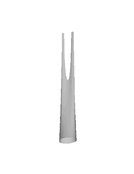
FIG. 2.: The “pair of pants” upside down – corresponding to a fissioning white hole. The image shows a $x=0$ slice of the null surface generated from the parameter set BBH (see table I) and was produced with the method described in Sec. III C. Spatial cuts of this null surface are shown in Figs. 6 – 8.

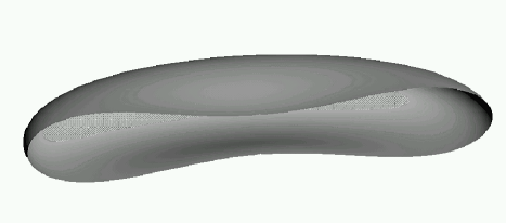
FIG. 3.: Spatial cut of the event horizon for the model QS at affine time $t=1.78$. At this early stage, the wavefront corresponds qualitatively to the oblate spheroidal case. The surface is clearly bulged inwards, so the rays at the poles of the event horizon cross first, but the deviation from axisymmetry is not yet apparent.

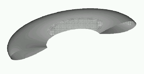
FIG. 4.: Spatial cut of the event horizon for model QS at affine time $t=1.90$. After the rays at the poles of the event horizon have crossed, the event horizon becomes a torus, losing points at a sharp inner edge which is a cut of the crossover surface.

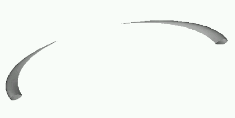
FIG. 5.: Spatial cut of the event horizon for model QS at affine time $t=2.5$. In the absence of axisymmetry some of the circles on the torus which link the hole pinch off to zero faster than others – the toroidal white hole fissions into two white hole fragments. After the fissioning, two “pincers” have formed between the sections, their tips are caustic points.

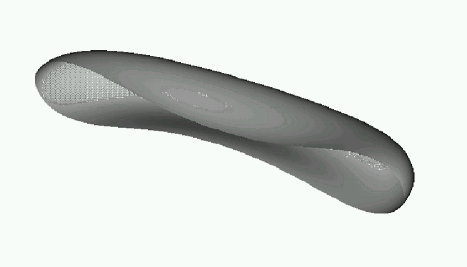
FIG. 6.: Model BBH at an early time $t=5.17$. The surface corresponds qualitatively to Fig. 3 from the quasispherical evolution but is now prolate instead of oblate.

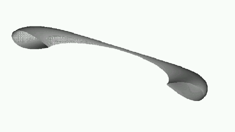
FIG. 7.: Model BBH at time $t=10.6$, when the event horizon is in its toroidal phase.

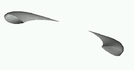
FIG. 8.: Model BBH at time $t=12.25$, after the event horizon has fissioned into two components.

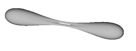
FIG. 9.: Highly prolate model BBH2 at time $t=11.8$ showing the toroidal phase. In the axisymmetric prolate limit the hole in the torus shrinks to zero.

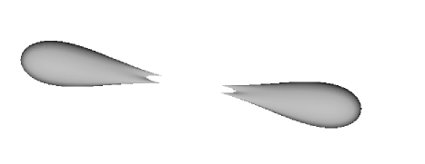
FIG. 10.: Highly prolate model BBH2 at time $t=13.1$ showing two individual white holes. In the axisymmetric prolate limit the pincers merge into “tips” of the “teardrops”.

REFERENCES

- [1] S. Shapiro and S. Teukolsky, Phys. Rev. D45, 2739 (1992).
- [2] P. Anninos, D. Hobill, E. Seidel, L. Smarr, and W.-M. Suen, Phys. Rev. Lett. 71, 2851, (1993).
- [3] S. A. Hughes, C. R. Keeton, P. Walker, K. Walsh, S. L. Shapiro, and S. A. Teukolsky, Phys. Rev. D49, 4004 (1994).
- [4] A. M. Abrahams, G. B. Cook, S. L. Shapiro, and S. A. Teukolsky, Phys. Rev. D D49, 5153 (1994).
- [5] P. Anninos, D. Bernstein, S. Brandt, J. Libson, J. Massó, E. Seidel, L. Smarr, W.-M. Suen, and P. Walker, Phys. Rev. Lett. 74, 630 (1995).
- [6] J. Libson, J. Massó, E. Seidel, L. Smarr, W-M Suen, P. Walker, Phys. Rev. D 53, 4335 (1995).
- [7] L. Lehner, N. T. Bishop, R. Gómez, B. Szilágyi, and J. Winicour, Exact Solutions for the Intrinsic Geometry of Black Hole Coalescence, to appear in Phys. Rev. D15, available from the Los Alamos preprint repository as gr-qc/9809034.
- [8] R. A. Matzner, H. E. Seidel, S. L. Shapiro, L. Smarr, W-M Suen, S. A. Teukolsky, and J. Winicour, Science 270, 941 (1995).
- [9] J. Massó, E. Seidel. W-M Suen and P. Walker, “Event Horizons in Numerical Relativity II: Analyzing the Horizon”, Phys. Rev D 59, March 15 (1999).
- [10] S. W. Hawking and G. F. R. Ellis, The Large Scale Structure of Spacetime (Cambridge University Press, Cambridge, 1973).
- [11] C. W. Misner, K. S. Thorne and J. A. Wheeler, Gravitation (W. H. Freeman, San Francisco, 1973).
- [12] R. Wald, General Relativity (University of Chicago Press, Chicago, 1984).
- [13] R. Thom, (1972) English translation, Structural Stability and Morphogenisis (Benjamin, Reading, Mass., 1975).
- [14] V. I. Arnold, (1974) English translation, Mathematical Methods of Classical Mechanics (Springer-Verlag, NY, 1978).
- [15] M. V. Berry and C. Upstill, Progress in Optics, XVIII, 256 (1980).
- [16] S. Shapiro, S. Teukolsky and J. Winicour, Phys. Rev. D52, 6982 (1995).
- [17] M. Siino, Phys. Rev. D 59, 064006 (1999).
- [18] P. M. Morse and H. Feshbach Methods of Mathematical Physics, pt. I (McGraw Hill, NY, 1973).
- [19] R. K. Sachs, J. Math. Phys. 3, 908 (1962).
- [20] H. Friedrich, Proc. Roy. Soc. Lond. A375, 169 (1981).
- [21] H. Friedrich, Proc. Roy. Soc. Lond. A378, 401 (1981).
- [22] S. A. Hayward, Class. Quantum Grav. 10, 779 (1993).
- [23] R. Piessens et. al., Quadpack: a subroutine package for automatic integration, (Springer-Verlag, Berlin, NY, 1983).
- [24] R.W. Brankin, I. Gladwell and L.F. Shampine, ‘RKSUITE: a Suite of Runge-Kutta Codes for the Initial Value Problem for ODEs”, Softreport 92-S1, Math. Dept., Southern Methodist University, Dallas, Texas, U.S.A, 1992, (also available by anonymous ftp from Southern Methodist University and from netlib in directory ode/rksuite).
- [25] R.W. Brankin and I. Gladwell, ‘A Fortran 90 Version of RKSUITE: An ODE Initial Value Solver”, Annals of Numer. Math., 1 (1994), 363-375.
- [26] N.T. Bishop, R. Gómez, L. Lehner, and J. Winicour, Phys. Rev. D, 54 6153, 1996.
- [27] N. T. Bishop, R. Gómez, L. Lehner, M. Maharaj and J. Winicour, Phys. Rev. D,56 6298 (1997).
- [28] R. Gómez, L. Lehner, R. Marsa, and J. Winicour, Phys. Rev. D 57, 4778 (1997).
- [29] S. W. Hawking, Commun. Math. Phys., 25, 152 (1972).
- [30] M. Spivak A Comprehensive Introduction to Differential Geometry Vol. III (Publish or Perish, Berkely, 1979).
- [31] D. Gannon, Gen. Rel. Grav. 7, 219 (1976).
- [32] P.T. Chruściel and R.M. Wald, Class. Quantum Grav. 11 L147 (1994).
- [33] G. J. Galloway, in Differential Geometry and Mathematical Physics, Contemp. Math., eds. J. Beem and K.L. Duggal 170, 113 (Amer. Math. Soc., Providence, 1994).
- [34] T. Jacobson and S. Venkataramani, Class. Quantum Grav. 12, 1055 (1995).
- [35] S. Browdy and G. J. Galloway, J.. Math. Phys. 36, 4952 (1995).
- [36] G. J. Galloway, Class. Quantum Grav. 12, L99 (1995).
- [37] M. Siino, Phys. Rev. D 58, 104016 (1998).
- [38] J. L. Friedman, K. Schleich, and D. M. Witt, Phys. Rev. Lett. 71, 1486 (1993).