Time-Frequency Detection of Gravitational Waves

Abstract

We present a time-frequency method to detect gravitational wave signals in interferometric data. This robust method can detect signals from poorly modeled and unmodeled sources. We evaluate the method on simulated data containing noise and signal components. The noise component approximates initial LIGO interferometer noise. The signal components have the time and frequency characteristics postulated by Flanagan and Hughes for binary black hole coalescence. The signals correspond to binaries with total masses between $45M_{\odot}$ to $70M_{\odot}$ and with (optimal filter) signal-to-noise ratios of 7 to 12. The method is implementable in real time, and achieves a coincident false alarm rate for two detectors $\approx$ 1 per 475 years. At this false alarm rate, the single detector false dismissal rate for our signal model is as low as 5.3% at an SNR of 10. We expect to obtain similar or better detection rates with this method for any signal of similar power that satisfies certain adiabaticity criteria. Because optimal filtering requires knowledge of the signal waveform to high precision, we argue that this method is likely to detect signals that are undetectable by optimal filtering, which is at present the best developed detection method for transient sources of gravitational waves.

I Introduction

According to Thorne[1], gravitational wave (GW) astronomy “will create a revolution in our view of the universe comparable to or greater than that which resulted from the discovery of radio waves.” He further asserts that “when gravitational waves are finally seen, they will come predominantly from sources we have not thought of or we have underestimated.” It follows that GW data analysis tools should include detection methods for poorly modeled and unmodeled signal waveforms.

However, at present the only well-characterized method being widely implemented for the detection of GWs from burst or transient sources is Wiener’s optimal filter [2]. This is a natural choice for sources whose signal waveforms are theoretically well modeled, because it is the optimal linear detection algorithm for such waveforms [3]. Unfortunately, the effectiveness of optimal filtering is greatly reduced by errors in the predicted signal waveform. Furthermore, even small errors in GW source modeling can lead to large cumulative errors in the predicted waveform [4]. Optimal filtering is therefore a poor technique for inadequately modeled (or unmodeled) sources. In fact, only two potential GW sources, binary inspiral and black hole quasi-normal ringdown, are thought to be adequately modeled for this method to work. Clearly, a method whose effectiveness is only weakly dependent on (or perhaps independent of) prior knowledge of the signal is needed. We call such methods “robust.”

One class of robust techniques widely used for signal analysis is time-frequency (TF) methods (cf. [5]). The central idea is straightforward: one simultaneously decomposes the data in two bases, time and frequency. The resulting distribution, $\rho(t,f)$, represents the energy of the data waveform at time $t$ and frequency $f$.

Time-frequency methods are well suited to analyzing interferometric gravitational wave data. Since interferometers are broad band instruments, the noise energy will be distributed throughout the TF plane. GWs, on the other hand, are caused by bulk motions of matter and energy, and their spectra tend to be peaked about characteristic frequencies determined by the source dynamics. GW signals may therefore be identified as ridges in the surface $\rho(t,f)$. While preliminary investigation of time-frequency methods for GW data[6, 7, 8, 9, 10] show promise, to date we know of no complete TF detection method that has been implemented and evaluated.

This article describes and evaluates a time-frequency method for interferometric GW data analysis. The method has three steps:

1. transform the interferometer data into a Wigner-Ville TF distribution $\rho(t,f)$ (described in Section II),

2. search for ridges in $\rho(t,f)$ using Steger’s algorithm (described in Section III),

3. threshold on length of ridge to eliminate false alarms.

We find this algorithm can reliably detect weak signals in simulated data with minimal assumptions about the signal.

Our evaluation of the TF method (Section V) consists of estimating false alarm and false dismissal probabilities for a variety of signals. False alarm probabilities are estimated by applying the method to a large number of data segments containing only simulated initial LIGO detector noise and simply counting detections. For false dismissal probability estimates, the same procedure is performed on data containing both simulated initial LIGO noise and simulated intermediate-mass ($22.5M_{\odot}-22.5M_{\odot}$ to $35M_{\odot}-35M_{\odot}$) binary black hole coalescence (BBHC) waveforms. These waveforms are an appropriate testing ground for robust methods, since they are probably dominated by the poorly understood merger signal. Furthermore, the recently discovered possible evidence of “middleweight” black holes[11, 12] implies that these may be important sources of GWs. Flanagan and Hughes[13] have estimated the duration and frequency band of the merger signal, and our test waveforms are constructed to conform to these estimates (see Appendix A for details). Thus, while our model waveform is not the correct signal for a BBHC, we believe it has the correct general characteristics for our evaluation.

The results of our evaluation are promising. We obtain a false alarm rate of one per 3.4 hours in a single detector, or approximately one per 475 years for coincident detection in the two LIGO 4 km detectors. Here, coincident means that signals are detected in both detectors within a certain time interval, or coincidence window. The coincidence window is taken to be 0.01 seconds (the light travel time between the LIGO 4 km detectors), since that is the maximum time interval between the arrival of a single gravitational wave (which travels at the speed of light) at these two detectors. False dismissal rates vary with the signal-to-noise ratio (SNR) (as measured by an optimal filter, cf. [2]) and binary mass, but as an example we find that approximately 3% of signals are lost at an SNR of 11 for a $30M_{\odot}-30M_{\odot}$ BBHC. Graphs showing false dismissal rates as a function of binary mass for a range of SNRs and as a function of SNR for a range of binary masses are presented in Section V. This TF method is also computationally efficient; we are able to analyze data in these simulations at about twice the acquisition rate of the simulated data.

While we are encouraged by these results, there is much more research to be done. We have restricted our attention in this paper to a single TF distribution (Wigner-Ville), a single ridge detection scheme (Steger’s algorithm), and a single thresholding scheme (ridge length). For each of these there are a variety of choices available, and these choices need to be explored and evaluated. We have also restricted our attention to only BBHC signal models, and only for a limited binary mass range. While we feel that these are priority targets for such a robust search method, there are other sources which should be investigated. A more complete description of these and other issues for future research are presented in Section VI.

II The Wigner-Ville Distribution

A Time-Frequency Distributions

The central idea of TF methods is to convert time domain data, $h(t)$, into a time-frequency distribution (TFD) $\rho(t,f)$. Here, the variable $f$ labels the basis vectors in an alternative basis which spans the Hilbert space to which $h(t)$ belongs (i.e. alternative to a basis labeled by $t$). This alternative basis is usually the frequency basis associated with the Fourier representation of $h(t)$, although it need not be (e.g. when wavelet bases are used). Likewise, the meaning of $\rho(t,f)$ varies, although it is usually associated in some way with the squared magnitude of $h$ at time $t$ and frequency $f$.

Methods for constructing $\rho(t,f)$ can be divided into two broad categories[14]: atomic decompositions such as windowed Fourier transforms and wavelet transforms and bilinear distributions of the form

$$\rho(t,f)=\int\int h(u)~{}h^{*}(v)~{}W(u,v;t,f)~{}du~{}dv$$ (1)

where $*$ denotes complex conjugation and the kernel $W$ satisfies

$$\int\int W(u,v;t,f)~{}dt~{}df=\delta(u-v).$$ (2)

Both types of TFD might in principle be used to detect gravitational waves.

The choice of a suitable TFD is governed by two requirements. The first is that the TFD must have good time-frequency localization properties. By this we mean the following: if a signal written in the form $h(t)=A(t)\cos\varphi(t)$ (with $\varphi(t)$ a continuously differentiable monotonic function) satisfies the adiabaticity conditions

$$A\left(\rule{0.0pt}{11.38109pt}t+\delta(t)\right)\approx A(t),$$ (3)

$$\dot{\varphi}\left(\rule{0.0pt}{11.38109pt}t+\delta(t)\right)\approx\dot{\varphi}(t),$$ (4)

where $\delta(t)$ is defined by $\varphi\left(\rule{0.0pt}{11.38109pt}t+\delta(t)\right)=\varphi(t)+2\pi$ for all $t$, then it should give rise to a distribution $\rho(t,f)$ which has support only in a small neighborhood of the curve $f=\dot{\varphi}(t)$. In other words, if the signal has a well defined frequency at each time, then the TFD should reflect that. This is required for a ridge detection algorithm to work well with the TFD. The second requirement is that the TFD be relatively inexpensive to compute. This makes real-time analysis of interferometer data feasible.

Gonçalves, Flandrin and Chassande-Mottin[6] have investigated the localization properties of various TFDs when applied to binary inspiral chirp waveforms. They conclude that bilinear distributions have superior localization properties, and we therefore focus our attention on those. On the other hand, bilinear distributions can be computationally expensive, depending on the choice of kernel $W$ in (1). The question, then, is whether there is a kernel for which $\rho$ can be calculated efficiently.

B The Wigner-Ville Distribution

There is at least one choice of kernel which leads to a computationally efficient bilinear distribution with good localization properties: the Wigner-Ville distribution (WVD)[15, 16]

$$\rho(t,f)=\int_{-\infty}^{\infty}h^{*}\left(t-\frac{\tau}{2}\right)h\left(t+\frac{\tau}{2}\right)e^{i2\pi f\tau}d\tau.$$ (5)

We will use the WVD , but note that it exhibits two features that might at first glance seem undesirable.

Both features are illustrated by considering a purely sinusoidal signal, $h(t)=\sin(2\pi f_{0}t)$. The WVD for this $h(t)$ is

$$\rho(t,f)=\frac{1}{4}\left[\delta(f-f_{0})+\delta(f+f_{0})-2\cos(4\pi f_{0}t)\delta(f)\right].$$ (6)

First, note that $\rho(t,f)$ does not have support only at the sinusoid’s frequency $f=\pm f_{0}$, but also has an “echo” at $f=0$. The sum of two sinusoids $h(t)=\sin(2\pi f_{1}t)+\sin(2\pi f_{2}t)$, has further echoes at $f=\pm(f_{1}\pm f_{2})$. These echos are due to the bilinearity of the distribution. Second, observe that this $\rho(t,f)$ attains negative values at $f=0$ whenever $\cos(4\pi f_{0}t)$ is positive. Thus, it is not entirely correct to think of the $\rho(t,f)$ as the squared magnitude of the signal at a give time and frequency.

Despite this behavior, the WVD is well suited to our method. We wish to look for ridges in the TF plane. Negative values away from these ridges are of no consequence. In fact, throughout this paper we will adopt the convention of setting negative values of $\rho(t,f)$ to $0$. Also, since we are interested only in detection here, and not in extracting information about the signal, it does not matter how many ridges there are in the TFD, it matters only that their existence be highly correlated with the presence of a signal and that they be sharp. The WVD satisfies both these criteria.

C Discrete Implementation

While the discussion above has been couched in the language of functions of continuous variables, in practice it is necessary to calculate WVDs from discretely sampled data $h_{j}=h(j\Delta t)$. This appears to presents a minor dilemma, since (5) contains expressions of the form $h(t-\tau/2)$, which when discretized become $h_{j-k/2}$. For interferometer data, this issue is easily dealt with, since the data will be significantly ($\sim$ 10 times) oversampled. It is thus a simple matter to decimate these data to twice the time resolution required. We resample our simulated data so that $h_{j}\equiv h(2j\Delta t)$ accordingly.

A second issue (also present in the continuous case) is that in practice $h(t)$ is known only in a time interval $0\leq t\leq T$. This means that $h(t-\tau/2)$ is undefined for $\tau/2>t$, and likewise $h(t+\tau/2)$ for $\tau/2>T-t$. In order to calculate (5) one must assign values to $h(t)$ in the entire time interval $-\infty\leq t\leq\infty$. We therefore take $h(t)=0$ in the intervals $t<0$ and $t>T$.

Having resolved these issues, it is straightforward to calculate the discrete analog of (5)

$$\rho_{jk}=\sum_{\ell=-N/2}^{N/2}~{}h_{(j-\ell/2)}~{}h_{(j+\ell/2)}~{}e^{2\pi ik\ell/N},$$ (7)

where $N=T/\Delta t$. This discrete distribution can be treated as a digital image, with $j$ and $k$ respectively denoting the horizontal and vertical pixel number. The value of $\rho_{jk}$ denotes the gray scale value, or equivalently height (i.e. $z$ value), of the image in that pixel.

It is easy to estimate the computational efficiency of the discrete WVD from (7). For each value of $j$, one does a single multiplication (of negligible cost) and a Fourier transform. The Fast Fourier transform costs $N\log_{2}(N)$ floating point operations, and must be done for each of $N/2$ possible values of $j$. Thus, the cost of calculating the WVD is approximately $(N^{2}\log_{2}N)/2$.

Finally, note that for a data set with $N$ samples the resulting WVD has $N^{2}/8$ pixels ($N/2$ time intervals by $N/4$ positive frequency bins). Images from large data sets therefore quickly become unwieldy; for example the data sets we used contained 4096 floats, leading to an image of $2048\times 1024$ pixels. We therefore averaged over 4 pixel intervals in time and 2 pixel intervals in frequency to obtain a more wieldy image size of $512\times 512$.

We end this Section with an example of a discrete Wigner-Ville TFD. Figure 1 shows two WVDs: one of simulated initial LIGO noise and the other of a simulated BBHC waveform embedded in that same noise (see Section V A and Appendix A for details).

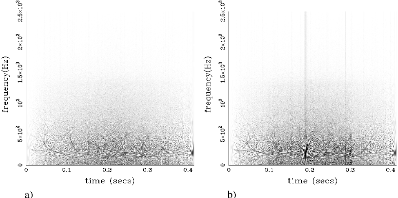
FIG. 1.: The WVDs of a) simulated initial LIGO noise and b) a simulated signal and noise (optimal filter SNR=8). In both cases, the data is over-whitened (see Section V). In this figure, the darkness of a pixel corresponds to the magnitude of $\rho(t,f)$ in that pixel, with darker pixels having higher values. Thus, a dark curve corresponds to a ridge in the distribution. In b), the signal, which is a model binary black hole coalescence waveform, is the dark structure in the bottom center (at about 0.2 sec) of the figure. The additional structure in the figures is self interference due to the bilinearity of the Wigner-Ville distribution.

III Steger’s Ridge Detection Algorithm

A gravitational wave signal in interferometer data $h(t)$ should produce a ridge in the TFD $\rho(t,f)$. Therefore, to detect GWs, a ridge detection algorithm (or equivalently line detection algorithm if $\rho(t,f)$ is represented as a gray-scale map as in Fig. 1) is required. Fortunately, there are a number of ridge detection algorithms in the digital image processing and computer vision literature from which to choose [17].

We use Steger’s second-derivative hysteresis-threshold algorithm [18]. The essential idea of this scheme is simple. A ridge in a surface will have high curvature (second derivative of $\rho(t,f)$) in the direction perpendicular to the ridge. Furthermore, the first derivative will vanish at the top of the ridge, since it is a local maximum. Thus, ridges are identified as contiguous sets of point at which $\rho(t,f)$ has a high-curvature local maximum.

Steger’s algorithm, which identifies ridges in this way, has a number of steps. First the TFD $\rho(t,f)$ is convolved with a 2-dimensional Gaussian smoothing kernel,

$$K(t,f)=\frac{1}{2\pi\sigma^{2}}~{}e^{-\frac{1}{2}\left[\left(\frac{t}{\sigma t_{p}}\right)^{2}+\left(\frac{f}{\sigma f_{p}}\right)^{2}\right]},$$ (8)

where the dimensionless scale parameter $\sigma$ allows the preferential detection of ridges of width $\stackrel{{\scriptstyle<}}{{\sim}}$ $\sigma t_{p}$ or$\sigma f_{p}$ , and the parameters $t_{p}$ and $f_{p}$ are characteristic time and frequency scales of the TFD (we used $t_{p}=4\Delta t$ and $f_{p}=2/T$, the time and frequency resolution of the digitized $\rho(t,f)$). One then takes the the first and second derivatives of the convolution

$$H(t,f)=\int^{\infty}_{-\infty}\int^{\infty}_{-\infty}\rho(t^{\prime},f^{\prime})K(t-t^{\prime},f-f^{\prime})~{}dt^{\prime}df^{\prime},$$ (9)

with respect to both $t$ and $f$. The second derivatives are used to find the eigenvectors $(n_{t},n_{f})$ of the Hessian matrix,

$$\left(\begin{array}[]{cc}\frac{\partial^{2}}{\partial t^{2}}&\frac{\partial^{2}}{\partial t\partial f}\\ \frac{\partial^{2}}{\partial f\partial t}&\frac{\partial^{2}}{\partial f^{2}}\end{array}\right)H(t,f)\left(\begin{array}[]{c}n_{t}\\ n_{f}\end{array}\right)=\alpha\left(\begin{array}[]{c}n_{t}\\ n_{f}\end{array}\right).$$ (10)

At each point in the $t-f$ plane, the eigenvector corresponding to the largest eigenvalue magnitude, $|\alpha|$, defines the line in the $t-f$ plane along which the second derivative of $H(t,f)$ obtains its extremal value. For points on a ridge, these vectors will be normal to the curve described by the ridge in the $t-f$ plane. If the first derivative of $H(t,f)$ vanishes in this direction,

$$\left(n_{t}\frac{\partial}{\partial t}+n_{f}\frac{\partial}{\partial f}\right)H(t,f)=0,$$ (11)

then the point may be on a ridge. We call such points “potential ridge points”.

If all potential ridge points were included in ridges, one would find ridges everywhere in the TFD due to noise fluctuations, whether a signal was present or not. To avoid this, one thresholds on the value of the second derivative. However, thresholding presents conflicting requirements. On one hand, if the threshold is too low, it will allow too many noise ridges to be detected. On the other hand, if it is too high, portions of a genuine signal ridge may be missed due to deviations below the threshold caused by noise. To improve the detection of signal ridges while suppressing noise ridges, hysteresis thresholding is used. This means that there are two thresholds on the second derivative of $\rho$, an upper threshold, which must be exceeded by any point at which a ridge can start, and a lower threshold, which must be exceeded by every point on the ridge.

Finally, ridges are identified as contiguous sets of potential ridge points which meet the hysteresis thresholding criteria. Isolated potential ridge points are not defined to be ridges. Note that small gaps in a ridge will be “smeared out” when the TFD is convolved with the Gaussian kernel. Thus, gaps of less than a few $\sigma f_{p}$ or $\sigma t_{p}$ are overlooked by this algorithm, which decreases the probability of noise fluctuations breaking a signal ridge into many smaller ridges. Conversely, the minimum ridge length detected is also a few $\sigma t_{p}$ or $\sigma f_{p}$, eliminating many shorter noise ridges.

There are some further issues involved with implementing this algorithm on a digital image. When $t$ and $f$ are replaced by their discrete counterparts, $t_{j}$ and $f_{k}$, the distribution $\rho_{jk}=\rho(t_{j},f_{k})$ can be viewed as a piecewise constant function, having value $\rho_{jk}$ in the rectangle $[t_{j}-(\Delta t/2),t_{j}+(\Delta t/2)]\times[f_{k}-(\Delta f/2),f_{k}+(\Delta f/2)]$, where $\Delta t=t_{j}-t_{j-1}$ and $\Delta f=f_{k}-f_{k-1}$, and vanishing outside the image (i.e. when $j<0$ or $k<0$ and when $j>N$ or $k>N$). This piecewise constant function is then convolved with the continuous Gaussian kernel. The convolution is equivalent to the summation

$$H_{mn}=\sum_{j}\sum_{k}\rho_{jk}K_{(j-m)(k-n)},$$ (12)

where the convolution mask $K_{(j-m)(k-n)}$ is given by

$$K_{(j-m)(k-n)}=\int_{t_{j}-t_{m}-\Delta t}^{t_{j}-t_{m}+\Delta t}\int_{f_{k}-f_{n}-\Delta f}^{f_{k}-f_{n}+\Delta f}K(t,f)~{}dt~{}df.$$ (13)

Rather than taking discrete derivatives of $H$, the process can be made more efficient by using masks built from the derivatives of $K$. By integrating (9) by parts, one may see that the same result can be derived by either process. However, while the derivatives of $H$ need to be calculated at each step, the derivatives of $K$ can be calculated just once. Thus, along with (13), convolution masks are also made with $K$ replaced by its first and second derivatives with respect to $t$ and $f$.

Another issue addressed by Steger’s algorithm is the positioning of potential ridge points. For a digital image, the ridge will be composed of pixels within which the directional derivative (11) vanishes. A one dimensional example illustrates the method used to determine whether (11) is satisfied within a given pixel. Denote the one-dimensional image function by $f(x)$. Approximate $f(x)$ at a point $x_{j}$ by its second order Taylor series,

$$f(x)\approx f_{j}+\frac{1}{\Delta x}(f_{j+1}-f_{j-1})~{}(x-x_{j})+\frac{1}{2(\Delta x)^{2}}(f_{j-1}+f_{j+1}-2f_{j})~{}(x-x_{j})^{2},$$ (14)

where the coefficients are finite difference approximations of the derivatives of $f$ at $x_{j}$ and $\Delta x=x_{j+1}-x_{j}$. The derivative of (14) vanishes at $x=x_{j}+dx$ where

$$dx\equiv-\Delta x\left(\frac{f_{j+1}-f_{j-1}}{f_{j-1}+f_{j+1}-2f_{j}}\right).$$ (15)

This is within the $j^{th}$ pixel if and only if $x_{j}-\Delta x/2<x_{j}+dx<x_{j}+\Delta x/2$. In that case, $x_{j}+dx$ is considered to be a potential ridge point and the $j^{th}$ pixel is a “potential ridge pixel.” One then joins ridge pixels (as before) to find the ridge. The generalization to two dimensions is discussed in [18].

IV The Detection Method

We have thus far described two of the three steps in our GW detection method: generation of WVDs from interferometric data and the search for ridges (signals) in them. If all ridges corresponded to GW signals, the existence of a ridge would be an adequate detection statistic and these two steps would be sufficient. However, even after hysteresis thresholding (see Section III), stochastic detector noise will lead to spurious ridges in the WVD. This may be exacerbated if the noise is non-stationary and/or non-Gaussian, in which case signal ridges and noise ridges might have very similar characteristics. A more powerful statistic can be devised by thresholding on ridge characteristics which are more strongly correlated with signal ridges than with noise ridges. Of course, the more specific the threshold is to the signal, the less robust the detection technique will be.

Ridge length (i.e. the number of pixels in a ridge) is one characteristic which distinguishes signal ridges from noise ridges in stationary Gaussian noise. Since the noise is stochastic, it will produce a distribution of ridge lengths, with short ridges being more frequent than longer ones (e.g. see Fig. 3). The ridge length of a signal is (approximately) determined by the signal’s duration and frequency band. Thus ridge length is more strongly correlated with signal ridges than noise ridges, and setting a minimum ridge length threshold can further improve the detection statistic. Also, note that this thresholding is not so specific as to undermine the robustness of the TF method. For these reasons, we use ridge length as a threshold.

Our complete TF detection method consists of the following steps:

1. construct the Wigner-Ville distribution $\rho(t,f)$ of the detector output $h(t)$ as per Section II,

2. search for ridges in the TF map $\rho(t,f)$ using the Steger’s algorithm as per Section III

3. use a threshold on the length of the ridge as a detection criterion.

The remainder of this article evaluates the performance of this method.

V Signal Detection and False Alarm Statistics

The statistical performance of our TF method is measured by two probabilities: the probability of finding a signal when there is none, or false alarm probability and the probability of failing to find a signal when there is one, or false dismissal probability. These probabilities depend on the details of the noise and the signal.

A Noise and Signal Models

Our simulations were carried out with discretely sampled colored Gaussian noise. This noise was produced using the Numerical Recipes [19] routine gasdev(). We altered gasdev() to use the ran2() random number generator, since it produces much longer sequences of pseudo-random numbers than the default ran1() routine. We divided the unit-variance white Gaussian deviates produced by gasdev() into two equal sets, which were used as the real and imaginary components of the complex valued frequency domain noise data, $\tilde{n}_{j}$. Finally, we colored the noise data by multiplying them by the square root of the initial LIGO noise curve, $\tilde{n}_{j}\sqrt{S_{h}(|f|)}\rightarrow\tilde{n}_{j}$. The specific $S_{h}(|f|)$ we use is that of Abramovici et al. [20] as generated by the GRASP routine noise_power() with input parameter noise_file="noise_ligo_init.dat" [2].

The signal data was obtained by sampling a continuous waveform developed specifically to test this algorithm. This waveform simulates the signal from an intermediate-mass coalescing black hole binary. These are expected to be important sources whose gravitational waveforms cannot be calculated analytically in the initial LIGO sensitivity band. They are thus ideal candidates for a robust detection method. Our model is based on the predictions of Flanagan and Hughes [13]. We wish to emphasize that it is not intended to be “accurate” in the sense required for optimal filtering: rather, it is constructed to have time, frequency and energy characteristics consistent with the assumptions of [13]. Thus, the performance of our TF method for these simulated signals should be indicative of its performance for actual coalescence signals. A detailed description of the model waveform and its derivation is presented in Appendix A. A typical waveform (for a $30M_{\odot}-30M_{\odot}$ binary system) is shown in Fig. 2.

FIG. 2.: A simulated binary black hole coalescence waveform for a $30M_{\odot}$ - $30M_{\odot}$ system, showing the three phases of the coalescence described by Flanagan and Hughes [13]. The frequency of the wave increases monotonically. Only the portion of the waveform with frequency $\geq$ 40 Hz is shown.

B The Simulation Procedure

We analyzed simulated data in segments of $N=4096$ samples each. The assumed sampling frequency was $f_{s}=9868.420898$Hz (we chose the sampling frequency of the LIGO 40-meter prototype detector so that data from that detector could be easily analyzed). Each segment therefore lasts for $T=N/f_{s}\approx 0.415$ s, and the time interval between successive samples is $\Delta t=1/f_{s}\approx 1.013\times 10^{-4}$ s. Samples in each segment are denoted by $h_{j}=h(j\Delta t)$ where $j$ takes the values between $0$ and $4095$. We denote the Fourier transform of $h(t)$ by $\tilde{h}(f)$ and its discrete representation by $\tilde{h}_{j}=\tilde{h}(j\Delta f)$, where $\Delta f=1/T$ and $j$ takes the value between $0$ (DC) and $N/2$ (the Nyquist frequency).

We performed two types of simulations: one to determine false alarms probabilities (the probability that a signal is detected when none is present) and one to determine false dismissal probabilities (the probability that no signal is detected when one is present). In every simulation, the data stream contained Gaussian noise, as described in Subsection V A. To determine false alarm probabilities, no simulated signals were added, so that $\tilde{h}_{j}=\tilde{n}_{j}$. To determine false dismissal probabilities, simulated GW signals were added to the noise.

As indicated in Appendix A, the angle averaged signals were generated in the time domain. We therefore took the Fourier transform of the average signal, $\langle\tilde{h}^{\rm BBH}\rangle_{k}\equiv\sum_{j=0}^{N-1}e^{2\pi ijk/N}\langle h^{\rm BBH}\rangle_{j}$. The signal was normalized so that

$$\sum_{k=0}^{N/2}\frac{\left|\langle\tilde{h}_{\rm BBH}\rangle_{k}\right|^{2}}{(S_{h})_{k}}=1,$$ (16)

where $(S_{h})_{k}=S_{h}(k\Delta f)$ is the one-sided power spectrum of the noise. The frequency domain data stream is then taken to be,

$$\tilde{h}_{k}=\tilde{n}_{k}+{\rm SNR}\,\langle\tilde{h}^{\rm BBH}\rangle_{k},$$ (17)

where SNR is the signal-to-noise ratio obtainable by matched filtering.

Since the Wigner-Ville distribution is computed from the time series representation of the detector output, it was necessary to transform $\tilde{h}_{k}$ into the time domain. However, the power spectrum spans such a large dynamic range that significant numerical errors arise if one simply takes the inverse Fourier transform of $\tilde{h}_{k}$. We therefore “over-whitened” the data, $\tilde{h}_{k},\rightarrow\tilde{h}_{k}/(S_{h})_{k},$ to reduce the (time-domain) dynamic range. This procedure has the added benefit that it emphasizes the frequencies in which the detector is most sensitive while suppressing the frequencies where the noise is large. We then took the inverse Fourier transform of the over-whitened $\tilde{h}_{k}$, and subsequently computed its WVD, $\rho_{jk}\equiv\rho(j\Delta t,k\Delta f)$, as per Eq. (5).

This procedure produces discrete TFDs, whose dimensions may be expressed in units of pixels. Because of the undersampling involved in computing the discrete WVD (see Section II) we computed $\rho_{jk}$ at $4096/2=2048$ distinct offsets, giving the WVD a “width” of 2048 time pixels. Also, the transform is constructed only at positive frequencies up to the Nyquist frequency after undersampling. Thus, the WVD has a “height” of 1024 frequency pixels. The resulting TFDs had $2048\times 1024\approx 2\times 10^{6}$ pixels. This was too large for efficient computation, so we reduced the map size by averaging over every 4 time pixels and every 2 frequency pixels. The final discrete WVDs had dimension $512\times 512$ pixels, each pixel having area $0.0008s\times 9.6Hz=7.8\times 10^{-3}$.

Next, $\rho_{jk}$ was passed through Steger’s line recognition algorithm. We used Steger’s implementation of this algorithm[21], which assumes that the pixels of the image (distribution in our case) are unsigned characters, taking integer values between 0 and 255. To convert the floating point image $\rho_{jk}$ to its unsigned character analog ${(\rho^{b})}_{jk}$ it was necessary to rescale the data to fit in this range without saturating it. The scaling factor was calculated as follows: the maximum floating point value of $\rho_{jk}$ was found for each segment of noise data. The scaling factor was then chosen so that it scaled the average value of these maxima to the value 128. Once rescaled, the image was passed to Steger’s algorithm. The algorithm parameters we used were $\sigma=2$ and second derivative (hysteresis) thresholds of $10/{\rm pixel}^{2}$ and $3.33/{\rm pixel}^{2}$. Ideally, these values would be chosen by some optimization procedure, however, for this preliminary study they were selected “by hand” after extensive numerical experimentation.

For each map, the line recognition algorithm returns a list of ridges detected and their lengths. Our detection statistic was the length of the longest ridge in the map. Thus, a threshold value was chosen, and if this value was equaled or exceeded by the longest curve in a given map, a signal was said to have been detected in that map. For instance, if one chooses a threshold ridge length 30 pixels, a signal is said to have been detected in any map which contains a ridge whose length is 30 pixels or longer.

C False Alarm Probability

Our goal is an algorithm which has an acceptable false alarm rate $R_{f}$. In our case, this means determining a ridge length which is not equaled or exceeded in maps containing only noise more than once in every $1/R_{f}$ seconds. To compute this threshold, we simulated noise from an ensemble of statistically independent identical detectors. In our simulation, the ensemble consisted of approximately $1.7\times 10^{6}$ detectors, which corresponds to analyzing $1.7\times 10^{6}~{}\times~{}0.415$ seconds or about 196 hours of simulated data.

For each member of the ensemble, we computed a WVD. We then searched for ridges in the WVD using Steger’s algorithm and determined the length of the longest ridge. Ridges were found in 106 of the $1.7\times 10^{6}$ WVDs, or about 1 out of every $16\,000$ maps. In those maps in which ridges were found, the length of the longest ridge ranged from 7 to 68 pixels. The relative frequency with which the longest ridge had a length $\geq\ell$ pixels is shown as a function of $\ell$ in Figure 3.

FIG. 3.: The relative frequency with which Steger’s algorithm detected ridges with length $\geq\ell$ pixels in WVDs of simulated initial LIGO noise. Only the 106 maps in which ridges were detected are included in this graph. The unevenness of the graph is caused by statistical fluctuations due to small number statistics.

Based on this simulation we chose a ridge length threshold of 30 pixels. This threshold produces a false alarm probability of about $3.4\times 10^{-5}$, or a false alarm rate of about one every $3.4$ hours in a single detector. More interesting is the rate at which false alarms occur simultaneously in two uncorrelated detectors. This coincidence rate is proportional to the coincidence window $\tau$, i.e. the time interval within which the same signal can be seen by both detectors. A natural lower limit for $\tau$ is the light crossing time between detectors, $\tau_{c}$, since the time interval between the arrival of a single signal at the first detector and the last detector can be up to $\tau_{c}$. However, other considerations may set a larger $\tau$ for a given algorithm, leading to a higher coincident false alarm rate.

For the LIGO 4 km detectors, $\tau_{c}$ is approximately 10 ms. As implemented, the TF method did not resolve time-of-arrival to this accuracy, because we did not distinguish when in the 400 ms data segment the signal arrived. The coincidence window is therefore 400 ms, which corresponds to a coincident false alarm rate of approximately one 400 ms/(3.4 hr$)^{2}$, or about one per 12 years. However, recall that the time resolution of the WVD is less than 0.0008 s. Furthermore, recall that Steger’s algorithm identifies the position of ridges in the image (in fact, this feature was implemented in our code although we did not use it). Thus, at no extra computational cost, one could set $\tau=\tau_{c}=$ 10 ms. The TF method can therefore easily achieve a coincident false alarm rate of $10\,{\rm ms}/(3.4\,{\rm hr})^{2}$, or about one every $475$ years.

D False Dismissal Probabilities

The false dismissal probability depends on the nature and strength of the signal in the data. We’ve estimated these probabilities for simulated BBHC waveforms (Section V A). We used signals with SNRs (as measured by optimal filters) in the range 7 to 14. To demonstrate the robustness of this TF method we selected various coalescence waveforms corresponding to different binary system masses. We confined ourselves to the (total system) mass range $45M_{\odot}$ to $70M_{\odot}$. In this range the merger phase, for which the waveform cannot be calculated analytically, sweeps through the frequency band of maximum sensitivity for initial LIGO detectors, and dominates the detectable signal[13]. These are therefore masses for which robust methods will be most useful.

Figure 4 shows false dismissal probabilities as a function of binary mass at SNRs of 10, 12 and 14.

FIG. 4.: False dismissal probability as a function of mass. The three curves correspond to three different values the optimal filter signal-to-noise ratio. With the parameters we have chosen, our method tends to work better for higher mass binaries, where the energy is more localized in the TF map.

At an SNR of 14 the false dismissal rates are acceptable throughout the tested mass range. At an SNR of 10, however, more than 20% of signals are missed by our detection algorithm for system masses $\stackrel{{\scriptstyle<}}{{\sim}}$ $55M_{\odot}$. This is because as the mass of a system decreases, the proportion of the SNR which is attributable to the inspiral phase increases, as does the duration of the observable portion of the inspiral. Thus, the SNR of the signal is spread through a larger region of the TF map, leading to lower ridges and hence a loss of detectability.

In Figure 5 we plot the false dismissal probabilities versus the SNR for signals from $45M_{\odot},60M_{\odot}$ and $70M_{\odot}$ binary systems. Again, one sees in this Figure that high mass systems are more readily detected. False dismissal probabilities for every system mass decrease with signal-to-noise ratio as expected.

FIG. 5.: False dismissal probability as a function of SNR for three values of the total mass $M$ of the binary system for the model signal. Even at a modest SNR of 11, the false dismissal rate is below 50% for systems with masses between $70M_{\odot}$ and $45M_{\odot}$.

E Computational Efficiency

All our simulations were carried out on a 48 node Beowulf (parallel) computer comprised 300 MHz Alpha 21164 machines [22]. This computer can analyze 47 segments of data simultaneously (the 48th machine is used to coordinate the calculation). We found that we could apply our TF method to approximately $2\times 10^{4}$ data points per second (about twice the sampling rate of the simulated data).

For initial LIGO, the frequency band of maximum sensitivity is projected to be below a few hundred Hz[20]. Sampling rates of $\stackrel{{\scriptstyle<}}{{\sim}}$ 1024 Hz should therefore be sufficient to contain all signals detectable with this TF method. Thus, even modest parallel computing facilities could implement this method in real time for initial LIGO data.

VI Conclusion

A Summary

Optimal filtering has dominated the interferometric GW data analysis literature. This is because when one seeks signals of nearly exactly known form in stationary noise with known spectral density, optimal filters are the most sensitive linear filters. However, it is clear that there are sources of gravitational radiation that are not understood well enough to predict their signal waveforms. For such sources, matched filtering will not be a suitable detection method. It is therefore necessary to develop methods which can detect signals from poorly modeled or even unmodeled sources in interferometric GW data.

We have demonstrated that time-frequency methods may provide a tool for detecting such sources. Our method, with the parameters discussed above, produced an initial LIGO false alarm rate of $\approx(3.4~{}\mbox{hr})^{-1}$, which corresponds to coincident false alarm rate in two detectors of $\approx(475~{}\mbox{yr})^{-1}$. Our simulations also show that we reliably detect the postulated BBHC waveforms for binaries of various masses injected into the data at a variety of optimal filter signal-to-noise ratios. For instance, we detect 80% of signals with SNRs ranging from $\approx 8.8$ for higher mass binaries ($70M_{\odot}$) to $\approx 12.2$ for lower mass binaries ($45M_{\odot}$). These numbers are within a factor of two of those for optimal filtering of stellar mass binary inspirals, where for two detectors the detection threshold is usually taken to be an SNR of $\approx 6$ [23]. Furthermore, this method is implementable in real time with a realistic computing budget.

B Future Directions

While this method shows considerable promise, there are still a number of issues which must be addressed in order to determine how useful TF methods will be in general:

  Utilization -

One might use TF methods as a filter to identify data which should be analyzed for the presence of signals using other techniques (i.e. in an hierarchical search), for detecting the signals themselves, or as a method for characterizing detector noise. This paper only addresses signal detection.

  Choice of Algorithm -

We have presented only one of many TF methods that could be implemented. We have used the Wigner-Ville distribution and Steger’s ridge detection algorithm, however there are a number of other TFDs (cf. [6]) and ridge detection algorithms (e.g. Hough transforms[24, 25] or the curve and edge detection algorithms cited in the introduction of [18]) which might prove suitable. As a detection statistic, energy along ridges, total ridge length in a map, or “bunching” of ridges might provide better detection statistics than maximum ridge length.

  Optimization -

We have made heuristic choices for operating values of the smoothing parameter $\sigma$ and the second derivative thresholds in Steger’s algorithm. It would be desirable to have a process which, given a specific type of GW signal, optimizes these parameters.

  Implementation -

It is unlikely that a single TF method is sufficiently robust to detect all types of unmodeled sources, which means that a set of TF methods should be used. It is also possible that TF methods are optimally implemented hierarchically. For example, one might have two detection statistics; one with an unacceptably high false alarm rate but low computational cost and another with prohibitive computational cost but a low false alarm rate. By applying the second statistic only to those TF maps in which a signal is detected with the first statistic, one could achieve both computational efficiency and acceptable false alarm rates.

  Comparison with Other Techniques -

We do not know how TF methods compare to other techniques. Signals that are optimal for TF detection produce regions of high density in the TFD. For our simulated signals, this high density region spans relatively short time scales ($\approx 0.2$ s). They might therefore be equally well detected with much simpler time-series thresholding techniques such as the one described in [26]. We have investigated this possibility by comparing each datum used in our TF simulations to a threshold. We chose the threshold to produce the same false alarm rate as obtained with the TF method. This technique produced a false dismissal rate of about twice that of the TF method. However, it is unknown whether a more sophisticated time-series threshold or a different statistic such as the excess power statistic [27] would prove superior to the TF method.

There is one further issue which pertains to all robust methods. In order to detect a signal of unspecified form in noise, the noise must be well characterized. We have assumed Gaussian noise in this paper. It is uncertain at this time to what extent this assumption is valid, however it is known that noise from the LIGO 40 m prototype contains a significant non-Gaussian component. The extent to which this component can be identified and removed (perhaps with the aid of TF methods themselves) is an issue that will only be fully resolved once the relevant interferometer data becomes available.

Clearly, there is a much work to be done. Moreover, with interferometric detectors scheduled to begin taking data in approximately a years time, there is little time in which to do it. In an effort to expedite the resolution of the issues listed above, we have made our TF computer code available as part of the latest release of GRASP[2].

However, the results of this preliminary investigation are encouraging. With the resolution of these issues, TF methods promise to be useful tools for the detection of GW signals in interferometric data.

A The Binary Black Hole Coalescence Waveform

The signal waveforms we used in our false dismissal simulations are based on the description of binary black hole coalescence (BBHC) signals in Flanagan and Hughes (FH)[13]. They consist of three consecutive components: an inspiral component, a merger component, and a quasi-normal ringdown component. The division into these components is somewhat arbitrary. Roughly speaking:

• The inspiral component describes the evolution of the binary system up to the “innermost stable circular orbit” (ISCO). This component is well modeled for BBH systems of $\sim 1M_{\odot}$[28], but there is some doubt whether it is known well enough for optimal filtering for binaries of total mass $\stackrel{{\scriptstyle>}}{{\sim}}$ $20M_{\odot}$[29].

• The merger component describes the evolution of the system from ISCO until such time as the system can be described as a single perturbed Kerr black hole. No analytical descriptions of this component exist.

• The quasi-normal ringdown component describes the evolution of the system when it is well described as a single perturbed Kerr black hole. This component well modeled for all BBHC’s[30, 31].

In this Appendix, we model each component separately. The full coalescence waveform is then simply a combination of the three component waveforms:

$$\langle h^{\rm BBH}(t)\rangle=\left\{\begin{array}[c]{ll}\langle h^{\rm insp}(t)\rangle,&t<0,\\ A^{\rm merge}(t)~{}\cos\varphi^{\rm merge}(t),&0\leq t\leq t_{\rm merge},\\ \langle h^{\rm qnr}(t)\rangle,&t>t_{\rm merge},\end{array}\right.$$ (A1)

An example of such a waveform for a $30M_{\odot}$ – $30M_{\odot}$ system is shown in Figure 2. We use units in which $c=G=1$ throughout the remainder of this Appendix.

1 Quasi-Normal Ringdown

The ringdown waveform is given in [13] as

$$h_{+}^{\rm qnr}-ih_{\times}^{\rm qnr}=\frac{{\cal A}M}{r}~{}{}_{2}S^{2}_{2}(\iota,\beta,a)~{}e^{-2i\pi f^{\rm qnr}t-t/\tau+i\varphi_{0}}.$$ (A2)

Here, $M$ and $a$ are the mass and angular momentum per unit mass of the black hole, $r$ is the distance to the hole, ${}_{2}S^{2}_{2}(\iota,\beta,a)$ is a spin-weighted spheroidal harmonic, $f^{\rm qnr}$ is the characteristic frequency of the black hole normal mode, $\tau$ is the time constant for the exponential decay of the mode, $\varphi_{0}$ is an arbitrary phase factor, and $\iota$ and $\beta$ are angles that describe the orientation of the black hole’s spin axis with respect to the plane of the detector arms (c.f. Fig. 9.2 of [1]). This waveform is quite straightforward except for the presence of the spin-weighted spheroidal harmonic, ${}_{2}S^{2}_{2}(\iota,\beta,a)$.

This complication of the ${}_{2}S^{2}_{2}(\iota,\beta,a)$ factor is easily circumvented by considering only the root-mean-squared (RMS) average of it over the source orientation angles $\iota$ and $\beta$. When averaged in this way, spin-weighted spheroidal harmonic obeys the trivial relationship

$$\sqrt{\frac{1}{4\pi}\int d\Omega~{}\left|{}_{2}S^{2}_{2}(\iota,\beta,a)\right|^{2}}=\frac{1}{\sqrt{4\pi}}.$$ (A3)

Since we are not interested in modeling the waveform exactly (indeed, our point is to show that we can find even inaccurately modeled signals), let us for the sake of simplicity substitute the RMS value of $(4\pi)^{-1/2}$ for ${}_{2}S^{2}_{2}(\iota,\beta,a)$ in (A2) to obtain

$$\langle h_{+}^{\rm qnr}\rangle_{(\iota,\beta)}-i\langle h_{\times}^{\rm qnr}\rangle_{(\iota,\beta)}\equiv\frac{{\cal A}M}{\sqrt{4\pi}r}~{}e^{-2i\pi f^{\rm qnr}t-t/\tau+i\varphi_{0}}.$$ (A4)

Note that $\langle h_{+}^{\rm qnr}\rangle_{(\iota,\beta)}$ and $\langle h_{\times}^{\rm qnr}\rangle_{(\iota,\beta)}$ are not the $(\iota,\beta)$ angle averaged RMS values of $h_{+}^{\rm qnr}$ and $h_{\times}^{\rm qnr}$ respectively, but are rather the result of averaging ${}_{2}S^{2}_{2}$ over $(\iota,\beta)$.

From (A2), the detector response to the quasi-normal ringing of a black hole is obtained by

$$h(t)=F_{+}(\theta,\phi,\psi)h_{+}(t)+F_{\times}(\theta,\phi,\psi)h_{\times}(t),$$ (A5)

where $F_{+}$ and $F_{\times}$ are the beam pattern functions

$$F_{+}(\theta,\phi,\psi) = \frac{1}{2}(1+\cos^{2}\theta)\cos 2\phi\cos 2\psi-\cos\theta\sin 2\phi\sin 2\psi,$$ (A6)

$$F_{\times}(\theta,\phi,\psi) = \frac{1}{2}(1+\cos^{2}\theta)\cos 2\phi\sin 2\psi+\cos\theta\sin 2\phi\cos 2\psi,$$ (A7)

and $\theta$, $\phi$ and $\psi$ are angles which describe the detector orientation[1]. One may average over detector orientations to obtain

$$\left|h(t)\right|_{(\theta,\phi,\psi)} = \sqrt{\frac{1}{4\pi^{2}}\int_{0}^{\pi}d\theta\sin\theta\int_{0}^{2\pi}d\phi\int_{0}^{\pi}d\psi~{}h^{2}(t)},$$ (A8)

$$= \frac{1}{\sqrt{5}}\sqrt{h_{+}(t)^{2}+h_{\times}(t)^{2}}.$$ (A9)

Substituting (A4) into (A9) we get

$$A^{\rm qnr}(t)\equiv\left|\langle h(t)^{\rm qnr}\rangle_{(\iota,\beta)}\right|_{(\theta,\phi,\psi)}=\frac{{\cal A}M}{\sqrt{20\pi}r}e^{-t/\tau}.$$ (A10)

Notice that $A^{\rm qnr}(t)$ is no longer a waveform. The source angle averaging combines $h_{+}$ and $h_{\times}$ to in such a way that only the (exponentially decaying) amplitude envelope remains. To recover the waveform, we multiply $A^{\rm qnr}(t)$ by a cosine at the appropriate frequency,

$$\langle h(t)^{\rm qnr}\rangle \equiv A^{\rm qnr}(t-t_{\rm merge})~{}\cos(2\pi f^{\rm qnr}(t-t_{\rm merge})+\varphi_{0}^{\rm qnr}),$$ (A11)

$$= \frac{{\cal A}M}{\sqrt{20\pi}r}e^{-(t-t_{\rm merge})/\tau}\cos(2\pi f^{\rm qnr}(t-t_{\rm merge})+\varphi_{0}^{\rm qnr}).$$ (A12)

Here, the angle brackets serves to remind us that there have been two averaging processes used in obtaining this result, and we have offset the time variable $t$ by $t_{\rm merge}$ (the duration of the merger component) to facilitate combining it with the other waveform components as in (A1).

Finally, we wish to express (A12) in terms of the BBH system mass. Using Eq. (3.17) of [13] and the values $a=0.98$ and ${\cal A}=0.4$ quoted in Eq. (3.21) of [13], we have

$$f^{\rm qnr} = 1320{\rm Hz}\left(\frac{20M_{\odot}}{M}\right),$$ (A13)

$$\tau \approx \frac{11.63}{\pi f^{\rm qnr}}.$$ (A14)

Thus, the only free parameters remaining in (A12) are the system mass $M$, the time offset $t_{\rm merge}$ and the initial phase of the ringdown waveform $\varphi_{0}^{\rm qnr}$. The mass will remain a free parameter in our simulation, however $t_{\rm merge}$ and the initial phase are determined by the merger waveform.

2 Binary Inspiral

For the binary inspiral component, $h_{+}$ and $h_{\times}$ can be conveniently written in the form [1]

$$h^{\rm insp}_{+}(t) = -2\left(\frac{\mu}{r}\right)[\pi Mf^{\rm insp}(t)]^{2/3}(1+\cos^{2}\iota)\cos\varphi^{\rm insp}(t),$$ (A15)

$$h^{\rm insp}_{\times}(t) = -4\left(\frac{\mu}{r}\right)[\pi Mf^{\rm insp}(t)]^{2/3}\cos\iota~{}\sin\varphi^{\rm insp}(t),$$ (A16)

where $M=m_{1}+m_{2}$ is the total mass of the BBH system, $\mu=(m_{1}m_{2})/M$ is the reduced mass of the system, and $f^{\rm insp}(t)$ and $\varphi^{\rm insp}(t)$ are the binary inspiral orbital phase and frequency. These latter are given to first post-Newtonian order by[2]

$$f^{\rm insp}(t) = \frac{1}{8\pi M}\left\{\Theta^{-3/8}+\left(\frac{743}{2688}+\frac{11}{32}\eta\right)\Theta^{-5/8}\right\},$$ (A17)

$$\varphi^{\rm insp}(t) = \varphi_{\rm coal}-\frac{1}{\eta}\left\{\Theta^{5/8}+\left(\frac{3715}{8064}+{55}{96}\eta\right)\Theta^{3/8}\right\},$$ (A18)

where

$$\eta \equiv \frac{\mu}{M},$$ (A19)

$$\Theta \equiv \frac{\eta}{5M}(t_{\rm coal}-t).$$ (A20)

$\varphi_{\rm coal}$ and $t_{\rm coal}$ are the phase and time at which coalescence occurs (i.e. when the frequency becomes infinite). Note that inspiral waveforms are available to post-Newtonian order 2.5[2], but first post-Newtonian order will be sufficient for this crude model.

As with the ringdown waveform, we perform an RMS averaging over the source angles in the inspiral waveform. The equivalent averaging in this case replaces $(1+\cos^{2}\iota)/2$ in $h_{+}(t)$ and $\cos\iota$ in $h_{\times}(t)$ by their $(\iota,\beta)$ averaged RMS values,

$$\sqrt{\frac{1}{4\pi}\int d\Omega\left[\frac{1}{4}(1+\cos^{2}\iota)^{2}+\cos^{2}\iota\right]}=\frac{2}{\sqrt{5}},$$ (A21)

Thus,

$$\langle h^{\rm insp}_{+}(t)\rangle_{(\iota,\beta)} = -8\left(\frac{\mu}{\sqrt{5}r}\right)[\pi Mf^{\rm insp}(t)]^{2/3}\cos\varphi^{\rm insp}(t),$$ (A22)

$$\langle h^{\rm insp}_{\times}(t)\rangle_{(\iota,\beta)} = -8\left(\frac{\mu}{\sqrt{5}r}\right)[\pi Mf^{\rm insp}(t)]^{2/3}\sin\varphi^{\rm insp}(t),$$ (A23)

We also average over the detector orientations. Inserting (A22) and (A23) into (A9) and multiplying by $\cos\varphi^{\rm insp}(t)$ we have

$$\langle h^{\rm insp}(t)\rangle\equiv A^{\rm insp}(t)~{}\cos\varphi^{\rm insp}(t)=\frac{8\mu}{5r}[\pi Mf^{\rm insp}(t)]^{2/3}\cos\varphi^{\rm insp}(t).$$ (A24)

Again, we wish to express the waveform in terms of the system mass $M$. It therefore remains to fix the reduced mass $\mu$, the coalescence time $t_{\rm coal}$, and the coalescence phase $\varphi_{\rm coal}$. We restrict our attention to equal mass binaries, so that the reduced mass is therefore $\mu=M/4$. We fix $t_{\rm coal}$ so that the binary system attains the ISCO frequency, $f_{\rm ISCO}$, at time $t=0$, i.e. so that $f^{\rm insp}(0)=f_{\rm ISCO}$. Following [13], we use the Kidder-Will-Wiseman[32] value of $f_{\rm ISCO}=(20M_{\odot}/M)\times 205{\rm Hz}$. We also fix $\varphi_{\rm coal}$ so that the phase of the binary system vanishes at $t=0$, i.e. so that $\varphi^{\rm insp}(0)=0$. Note that this is not the same as choosing $t_{\rm coal}=0$ and $\varphi_{\rm coal}=0$, since coalescence occurs after the ISCO. This completes the specification (apart from the free mass parameter) of the inspiral component of the BBHC waveform.

3 Merger

The remaining task is to model the merger waveform. While no analytic model for the merger exists, Flanagan and Hughes[13] make educated estimates of some of its properties. They assume that the merger signal contains only frequencies between the ISCO frequency, $f_{\rm ISCO}$, and the quasi-normal ringing frequency, $f^{\rm qnr}$. They also estimate that the energy carried by the merger component of the wave is approximately $3$ times the energy carried by the quasi-normal ringdown component. Finally, they estimate the duration of the merger to be $t_{\rm merge}\sim 50M$. We use these criteria, along with the requirement that $h$ and $\partial_{t}h$ be continuous, to guide us in making a mock merger waveform. While the resulting waveform won’t be that of a real BBH merger, it should resemble it enough to determine whether our TF method can detect BBH waveforms for intermediate-mass systems.

The first step in our construction of a merger waveform estimate is to assume a form of

$$\langle h^{\rm merge}(t)\rangle=A^{\rm merge}(t)\cos\varphi^{\rm merge}(t).$$ (A25)

Continuity of the $f_{\rm merge}$ and $\partial_{t}f_{\rm merge}$ with both the inspiral waveform that proceeds it and the quasi-normal ringdown waveform that follows constitutes four conditions on $\varphi^{\rm merge}(t)$:

$$\frac{\partial\varphi^{\rm merge}}{\partial t}(t=0) = f_{\rm ISCO},$$ (A26)

$$\left(\frac{\partial^{2}\varphi^{\rm merge}}{\partial t^{2}}\right)(t=0) = \left(\frac{\partial^{2}\varphi^{\rm insp}}{\partial t^{2}}\right)(t=0),$$ (A27)

$$\frac{\partial\varphi^{\rm merge}}{\partial t}(t=t_{\rm merge}) = f^{\rm qnr},$$ (A28)

$$\left(\frac{\partial^{2}\varphi^{\rm merge}}{\partial t^{2}}\right)(t=t_{\rm merge}) = 0,$$ (A29)

where the last equation follows from the fact that the $f^{\rm qnr}$ is constant. To satisfy these four conditions will require a frequency model with four free parameter. We use the simplest such model; the merger frequency a cubic function of time. The phase is therefore a quartic of the form

$$\phi^{\rm merge}(t)=f_{\rm ISCO}t+\left(\frac{\partial^{2}\varphi^{\rm insp}}{\partial t^{2}}(0)\right)t^{2}+\varphi^{\rm merge}_{3}t^{3}+\varphi^{\rm merge}_{4}t^{4},$$ (A30)

where $\varphi^{\rm merge}_{3}$ and $\varphi^{\rm merge}_{4}$ can be obtained by solving (A28) and (A29) and we have set $\varphi^{\rm merge}(0)=0$. Once the merger phase polynomial has been determined, it is a simple matter to find the phase constant for the quasi-normal ringdown,

$$\varphi^{\rm qnr}_{0}=\varphi^{\rm merge}(t=t_{\rm merge}),$$ (A31)

which completes the specification of the quasi-normal ringdown component of the waveform.

To determine the merger amplitude function, we impose similar continuity conditions

$$A^{\rm merge}(t=0) = A^{\rm insp}(t=0)$$ (A32)

$$\left(\frac{\partial A^{\rm merge}}{\partial t}\right)(t=0) = \left(\frac{\partial}{\partial t}A^{\rm insp}\right)(t=0),$$ (A33)

$$A^{\rm merge}(t=t_{\rm merge}) = A^{\rm qnr}(t=t_{\rm merge}),$$ (A34)

$$\left(\frac{\partial A^{\rm merge}}{\partial t}\right)(t=t_{\rm merge}) = \left(\frac{\partial}{\partial t}A^{\rm qnr}\right)(t=t_{\rm merge}),$$ (A35)

We again need a fitting function with at least four parameters. However, there is a further constraint to impose; recall that [13] estimates the energy of the merger to be three times the energy of the quasi-normal ringdown, i.e.

$$\int_{0}^{t_{\rm merge}}\left(\frac{\partial}{\partial t}\langle h^{\rm merge}(t)\rangle\right)^{2}dt=3\int_{t_{\rm merge}}^{\infty}\left(\frac{\partial}{\partial t}\langle h^{\rm qnr}(t)\rangle\right)^{2}dt.$$ (A36)

This fifth condition on $A^{\rm merge}(t)$ requires a fifth parameter, and we therefore model the merger amplitude with a quartic,

$$A^{\rm merge}(t)=A^{\rm insp}(0)+\left(\frac{\partial}{\partial t}A^{\rm insp}\right)(0)~{}t+A^{\rm merge}_{2}t^{2}+A^{\rm merge}_{3}t^{3}+A^{\rm merge}_{4}t^{4},$$ (A37)

where the coefficients $A^{\rm merge}_{2,3,4}$ are determined by (A34), (A35) and (A36). This completes the specification of the merger waveform.

REFERENCES

- [1] K. S. Thorne, in 300 Years of Gravitation, edited by S. W. Hawking and W. Israel (Cambridge University Press, Cambridge, England, 1987), pp. 330 – 458.
- [2] B. Allen, GRASP: a data analysis package for gravitational wave detection, version 1.8.6 ed., Department of Physics, University of Wisconsin – Milwaukee, P.O. Box 413, Milwaukee WI 53201, USA, 1999, available at http://www.lsc-group.phys.uwm.edu/ballen/grasp-distribution/index.html.
- [3] L. A. Wainstein and V. D. Zubakov, Extraction of Signals from Noise (Prentice-Hall, Englewood Cliffs, N. J., 1962).
- [4] C. Cutler et al., Phys. Rev. Lett. 70, 2984 (1993).
- [5] Time-Frequency Signal Analysis, edited by B. Boashash (John Wiley & Sons, Inc., New York, 1992).
- [6] P. Gonçalvès, P. Flandrin, and E. Chassande-Mottin, in Second Workshop on Gravitational Wave Data Analysis, edited by M. Davier and P. Hello (Éditions Frotières, Gif Sur Yvette, France, 1998), pp. 35 – 46.
- [7] E. Chassande-Mottin and P. Flandrin, in Second Workshop on Gravitational Wave Data Analysis, edited by M. Davier and P. Hello (Éditions Frotières, Gif Sur Yvette, France, 1998), pp. 47 – 52.
- [8] J.-M. Innocent and B. Torrésani, in Second Workshop on Gravitational Wave Data Analysis, edited by M. Davier and P. Hello (Éditions Frotières, Gif Sur Yvette, France, 1998), pp. 53 – 64.
- [9] J.-M. Innocent and B. Torrésani, in Mathematics of Gravitation, edited by A. Królak (Banach Center Publications, Warsaw, 1997).
- [10] A. Królak and P. Trzaskoma, Class. Quantum Grav. 13, 813 (1996).
- [11] E. J. M. Colbert and R. F. Mushotzky, The Nature of Accreting Black Holes in Nearby Galaxy Nuclei, astro-ph/9901023.
- [12] A. Ptak and R. Griffiths, Hard X-ray Variability in M82: Evidence for a Nascent AGN?, astro-ph/9903372.
- [13] Éanna É. Flanagan and S. A. Hughes, Phys. Rev. D54, 4535 (1998).
- [14] P. Flandrin, in Wavelets: Time-Frequency Methods and Phase Space, edited by J. M. Combes, A. Grossman, and P. Tchamitchian (Springer Verlag, New York, 1987), pp. 68 – 98.
- [15] E. P. Wigner, Phys. Rev. 40, 749 (1932).
- [16] J. Ville, Cables et Transmission 2A, 61 (1948).
- [17] R. M. Harakick and L. G. Shapiro, Computer and Robot Vision (Addison-Wesley Publishing Company, Inc., New York, 1992), Vol. I.
- [18] C. Steger, IEEE Transactions on Pattern Analysis and Machine Intelligence 20, 113 (1998).
- [19] W. H. Press, S. A. Teulkosky, W. T. Vettering, and B. P. Flannery, Numerical Recipes in C, 2nd ed. (Cambridge University Press, Cambridge, England, 1992).
- [20] A. Abramovici et al., Science 256, 325 (1992).
- [21] C. Steger, computer code detect-lines 1.2, Technische Universitat München, München Germany, 1996, available at ftp://ftp9.informatik.tu-muenchen.de/pub/detect-lines/detect-lines-1.2.tar.gz.
- [22] More information on this computer system can be found at http://www.lsc-group.phys.uwm.edu/www/docs/beowulf/index.html.
- [23] C. Cutler and Éanna E. Flanagan, Phys. Rev. D49, 2658 (1994).
- [24] P. V. C. Hough, A Method and Means for Recognizing Complex Patterns, 1962, U.S. Patent No. 3,069,654.
- [25] R. O. Duda and P. E. Hart, Comm. ACM 15, 11 (1972).
- [26] N. Arnaud, F. Cavalier, M. Davier, and P. Hello, Detection of gravitational wave bursts by interferometric detectors, gr-qc/9812015.
- [27] W. G. Anderson, P. R. Brady, J. Creighton, and E. E. Flanagan, An excess power statistic for detection of burst sources of gravitational radiation, work in progress.
- [28] L. Blanchet, B. R. Iyer, C. M. Will, and A. G. Wiseman, Class. Quantum Grav 13, 575 (1996).
- [29] P. R. Brady, J. D. E. Creighton, and K. S. Thorne, Phys. Rev. D58, 061501 (1998).
- [30] S. A. Teukolsky and W. H. Press, Astrophys. J. 193, 443 (1974).
- [31] S. Chandrasekhar and S. L. Detweiler, Proc. R. Soc.London, Ser. A 344, 441 (1975).
- [32] L. E. Kidder, C. M. Will, and A. G. Wiseman, Phys. Rev. D47, 4183 (1993).