Operators for quantized directions

Abstract.

Inspired by the spin geometry theorem, two operators are defined which measure angles in the quantum theory of geometry. One operator assigns a discrete angle to every pair of surfaces passing through a single vertex of a spin network. This operator, which is effectively the cosine of an angle, is defined via a scalar product density operator and the area operator. The second operator assigns an angle to two “bundles” of edges incident to a single vertex. While somewhat more complicated than the earlier geometric operators, there are a number of properties that are investigated including the full spectrum of several operators and, using results of the spin geometry theorem, conditions to ensure that semiclassical geometry states replicate classical angles.

UWThPh - 1999 - 28

1. Introduction

Spin networks were first used by Penrose as a combinatorial foundation for Euclidean three-space [1]. When first defined, spin networks were non-embedded, trivalent graphs with spins assigned to every edge. Together with Moussouris, Penrose constructed a proof which demonstrated that the angles of three-dimensional space could be modeled by spin networks. This proof rests on conditions on the form of semiclassical states. They must be sufficiently correlated and the edges must have large spins. Penrose called this result the “spin geometry theorem.”

In 1994 spin networks were shown to be useful in the study of non-perturbative, canonical quantum gravity [2]. (See Ref. [3] for a recent review.) Since then, spin networks have become a key element in the kinematics of the theory. In fact, spin networks are the eigenvectors of operators which measure geometric quantities such as area and volume [4] - [6] and are a basis for the (kinematical) states of quantum gravity [7]. This collection of work is often described as loop quantum gravity or, emphasizing the kinematic level, quantum geometry [5]. Given these two spin network developments - the spin geometry theorem and the introduction of spin networks to quantum gravity - one might expect that there is a well-defined “angle operator” for quantum geometry. Such an operator exists and is defined in this paper.

In fact, I introduce several operators, two of which maybe be called “angle operators” and both of which directly lead to “quantized directions.” For each of these operators I define the quantum operators, compute the spectra, and then check the naive classical limit and construct a regularization. In so doing, the physical meaning and the interpretation of these operators becomes clear. The first cosine operator is defined in two stages. First, a scalar product density operator is introduced. Second, the scalar product operator is normalized by the point-wise areas of the two surfaces. The resulting operator - which is seen to give the cosine of the angle between the two surface normals - is a well-defined, self-adjoint operator on the space of kinematic states of quantum gravity. The second cosine operator and the associated angle operator are constructed with similar techniques but are based on “orthogonal” surfaces.

These steps are similar to the development of the “cosine operator” in Moussouris’ dissertation [9]. Since this work is unpublished, it is worth reviewing this construction in some detail. This is done in Section 2. In Section 3 there is a brief review of quantum geometry as it has developed in the background independent quantization of Hamiltonian gravity. In Section 4 a scalar product density operator is introduced and the spectrum computed. Then the cosine operator is defined. This operator is shown to have the expected naive classical limit in Section 4.4. There are two regularizations sketched in Section 4.5. In Section 5 the second angle operator is introduced. Some variations on the operator and the semiclassical limits are discussed in the final section of the paper. Both of the operators share some striking features including a completely discrete spectra and independence of both the Planck length and the Immirizi parameter ([10] - [12]).

2. The Spin Geometry Theorem

Difficulties inherent in the continuum formulation of physics – from ultra-violet divergences in quantum field theory to the evolution of regular data into singularities in general relativity – led Penrose to explore a fundamentally discrete structure for spacetime. His insight was that one could define the notion of direction with combinatorics of spin networks and recover the continuum of angles to arbitrary accuracy. He accomplished this by using the discrete spectrum of angular momentum operators.

Relative orientations arise out of a spin network structure through scalar products of angular momentum operators. The construction offers a way to determine angles in three dimensional space without any reference to background manifold structure. Realistic models of angles must be arbitrarily fine and are constructed with complex networks.

To see how this comes about, consider a spin state $\omega$ with $N$ correlated external lines as shown in Fig. (1a).

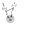
a	b	c

Figure 1. (a.) A spin network state with $N$ external lines based on the invariant $\omega$; a spin network with only these $N$ open lines. The lines are labeled $1,2,\dots,N$. Two of the spins $k$ and $l$ are identified. (b.) A particular example with two lines of $k$ and $l$ spin. (c.) The exchange of a spin-$1/2$ “particle.” This “experiment” helps determine the angle between the two lines.

These lines are built of $N$ ($N\geq 3$) spins $s_{i}$, $i=1,2,\dots N$. The relative angles between the different lines are described by angular momentum operators $\hat{J}_{(k)}$ which act on the $k$th line of the graph. (The indices in parentheses distinguish them from the indices of the spatial manifold.) The scalar product of two such spin operators is given by $\hat{T}^{(kl)}$

(1) $$\hat{T}^{(kl)}:=\hat{J}_{(k)}\cdot\hat{J}_{(l)}\equiv\sum_{i=1}^{3}\left(1\otimes\dots\otimes\hat{J}^{i}_{(k)}\otimes\dots\otimes\hat{J}^{i}_{(l)}\otimes\dots\otimes 1\right).$$

This operator acts non-trivially only on the two lines with spins $j_{k}$ and $j_{l}$. For instance, if $\hat{J}=\hat{J}_{(1)}+\hat{J}_{(2)}$, then the operator $\hat{T}^{(12)}$ may be written as

(2) $$\hat{T}^{(12)}=\tfrac{1}{2}\left[\hat{J}^{2}-\hat{J}_{(1)}^{2}-\hat{J}_{(2)}^{2}\right]$$

and has eigenvalues $\tfrac{1}{2}\left[j(j+1)-j_{1}(j_{1}+1)-j_{2}(j_{2}+1)\right]$. (Throughout this paper I denote scalar products with $T^{(\dots)}$.)

The spin geometry theorem states that for a sufficiently classical state $\omega$ the expectation values $\langle\omega\mid\hat{T}^{(kl)}\mid\omega\rangle\equiv\left\langle\hat{T}^{(kl)}\right\rangle_{\omega}$ model the scalar products of vectors in Riemannian 3-dimensional space. For states $\omega$ which are the direct product of unique polarization vectors the expectation value $\left\langle\hat{T}^{(kl)}\right\rangle_{\omega}$ is precisely the inner product of those polarization vectors [9].

In more detail, the interpretation of $\hat{T}^{(kl)}$ as scalar product of vectors requires a certain richness in the state $\omega$. Just as one must specify a set of conditions to find the Newtonian limit of general relativity, one must specify a set of classical limit conditions for these operators. These are the “classical constraints.” In the spin geometry theorem one has a choice of constraints based on the following scalar product lemma [9]: If $T^{(kl)}$ is a real, symmetric $N\times N$ matrix then these three conditions are equivalent:

1. There exist 3-dimensional vectors $\{\vec{v}\,{}^{k}\}$, $i=1,2,\dots N$, such that $T^{(kl)}$ is the scalar product, i.e. $T^{(kl)}=\vec{v}\,{}^{k}\cdot\vec{v}\,{}^{l}$.

2. $T^{(kl)}$ is positive, semi-definite of rank $\leq 3$.

3. $x_{k}\,T^{(kl)}\,x_{l}\geq 0$ for real $x_{k}$ and the determinants of all symmetric $4\times 4$ submatrices of $T^{(kl)}$ vanish.

The proof is an application of linear algebra [9].

In the quantum theory and for spins of finite magnitude, the classical constraints are only satisfied approximately. Hence, one says that a matrix $\left\langle\hat{T}^{(kl)}\right\rangle=T^{(kl)}$ satisfies the “$\epsilon$-constraints” if, for some $\epsilon>0$,

1. $T^{(kk)}>0$ and $x_{k}T^{kl}x_{l}\geq 0$ for real $x_{k}$ and

2. The matrix of cosines

   $$C^{(kl)}=\frac{T^{(kl)}}{2\left[T^{(kk)}T^{(ll)}\right]^{1/2}}$$

   satisfies

   $$\left|\det C^{(kl)}\right|^{1/2}<\epsilon$$

   when summing over $k,l$ in a 4-tuple of indices $K$. This condition requires that the four volume, defined by $K$, is less than $\epsilon$.

By the properties of symmetric matrices given above, spin operators $\hat{T}^{(kl)}$ satisfying these classical constraints approximate condition 3 above for real, symmetric matrices. This is how classical angles are approximated.

Quantum states can support this classical angle interpretation only when they are sufficiently correlated so that the geometric relations between spins give well-defined $\hat{T}^{(kl)}$’s. This condition is specified using a bound on the uncertainty. Defining the root-mean-square uncertainty in a state $\omega$ as

$$\sigma_{\omega}\hat{T}^{(kl)}:=\left[\left\langle\left(\hat{T}^{(kl)}-\left\langle\hat{T}^{(kl)}\right\rangle_{\omega}\right)^{2}\right\rangle_{\omega}\right]^{1/2},$$

$\hat{T}^{(kl)}$ is “$\delta$-classical” in the state $\omega$ when

$$\frac{\sigma_{\omega}\hat{T}^{(kl)}}{\|\hat{T}^{(kl)}\|}<\delta$$

where $\|\hat{T}^{(kl)}\|:={\rm sup}\{|\left\langle\hat{T}^{(kl)}\right\rangle_{\omega}|:\|\omega\|=1\}$. (For finite spins $\hat{T}^{(kl)}$ is a bounded operator, as can be seen from Eq. (2).) Since $\|\hat{T}^{(kl)}\|$ obtains the maximum value $j_{k}j_{l}$, the uncertainty $\sigma_{\omega}\hat{T}^{(kl)}/j_{k}j_{l}\leq\delta$. Thus, when the spins are large, the spin product operator $\hat{T}^{(kl)}$ models angles in 3-dimensional space.

The theorem is stated as

Theorem 1.

Spin Geometry Theorem: For all $\epsilon>0$, there exists a $\delta>0$ such that the values $\left\langle\hat{T}^{(kl)}\right\rangle_{\omega}$ satisfy the $\epsilon$-constraints for Riemannian 3-space, provided the observable $\hat{T}^{(kl)}$ is $\delta$-classical in the state $\omega$.

The proof may be found in Ref. [9] and only rests on the assumption that $\omega$ contains enough information to be $\delta$-classical (and the parameter $\delta$ is independent of the state $\omega$). In short, three dimensional angles are obtained if the state has two properties: Its spins must be large so the scalar products are fine enough to obtain the classical limit. And the state must be sufficiently correlated so there is enough information to separate random correlation from relative orientation.

Penrose proves a similar result using diagrammatic techniques which I sketch here. (See Refs. [1] and [9] for more detail.) One can consider a network with two free ends as in Fig. (1b). Penrose builds a new network by splitting off one line from the $s_{l}$ line and connecting it to the $s_{k}$ line. The two outcomes ($k\pm 1$) are shown in Fig.(1c). The cosine of the angle between the two edges $k$ and $l$ is defined to be the relative probability of the two outcomes. However, this is not sufficient. This angle is not the scalar product operator but also includes an “ignorance” factor. For instance, if the state $\omega$ was a set of uncorrelated lines then, in the limit of large spins, the two relative probabilities would become equal. If any angle was assigned in this case, it would have to be a right angle. Penrose fixes this ambiguity by making two successive measurements. If the resulting angles are approximately the same, then Penrose says the angle is well defined. Thus the cosine may be determined with

$$\mathchoice{\raisebox{-18.0pt}{ \psfig{height=40.0pt,silent={}} \hskip 2.0pt}}{\raisebox{-11.0pt}{\hskip 1.0pt \psfig{height=25.0pt,silent={}} \hskip 1.0pt}}{\raisebox{-10.0pt}{ \psfig{height=20.0pt,silent={}} \hskip 1.0pt}}{\raisebox{-8.0pt}{ \psfig{height=18.0pt,silent={}} }}\approx kl\cos\theta\mathchoice{\raisebox{-18.0pt}{ \psfig{height=40.0pt,silent={}} \hskip 2.0pt}}{\raisebox{-11.0pt}{\hskip 1.0pt \psfig{height=25.0pt,silent={}} \hskip 1.0pt}}{\raisebox{-10.0pt}{ \psfig{height=20.0pt,silent={}} \hskip 1.0pt}}{\raisebox{-8.0pt}{ \psfig{height=18.0pt,silent={}} }}.$$

The cosine may be calculated using recoupling theory. The relation between this approach and the scalar product can be seen rather directly. In brief, since $J^{i}=\tfrac{\hbar}{2}\sigma^{i}$ where $\sigma^{i}$ are the Pauli matrices and since [13]

(3) $$\frac{1}{2}\sum_{i=1}^{3}\sigma^{i\,B}_{A}\sigma^{i\,D}_{C}\equiv\mathchoice{\raisebox{-8.0pt}{ \psfig{height=24.0pt,silent={}} \hskip 2.0pt}}{\raisebox{-3.0pt}{\hskip 1.0pt \psfig{height=11.0pt,silent={}} \hskip 1.0pt}}{\raisebox{-2.0pt}{ \psfig{height=9.0pt,silent={}} \hskip 1.0pt}}{\raisebox{-1.0pt}{ \psfig{height=7.0pt,silent={}} }}$$

the angle is defined with a diagram identical to the one used in Eq. (1). Indeed, the angle is an eigenvector of the scalar product operator.

The spin geometry theorem shows that it is possible to build a classical-looking angle on a fundamentally combinatorial space. It is the limit which allows a fundamentally discrete spacetime to have classical properties. In this same manner, the spin geometry theorem offers lessons for the current formulation of quantum gravity. While the kinematic formulation is well understood and on rigorous footing, there is little notion of how to recover our familiar Minkowski spacetime. The subtleties encountered in the Spin Geometry Theorem surely have a reflection in the classical limit of non-perturbative quantum gravity.

With the spin geometry theorem as motivation, this paper introduces operators which lead to quantized directions. The idea is to, directly as possible, define angle operators for quantum geometry as they are defined in the spin geometry theorem. As the setting for these operators is quantum geometry, this is reviewed first.

3. Quantum Geometry: A brief review

In addition to a quick review of quantum geometry this section serves two purposes. It sets the framework of the operator definitions and serves to fix signs, factors, and units.

The quantum geometry framework is suitable for a class of gauge theories which are quantized with canonical, background metric-free methods. The notable example of such a theory is, of course, canonical quantum gravity. The kinematics of this theory is placed on an oriented, analytic three manifold $\Sigma$ which is compact (or the fields to be mentioned shortly satisfy appropriate asymptotic conditions). The classical configuration space $\cal{A}$ consists of all $su(2)$-valued smooth connections $A_{a}^{i}(x)$ on $\Sigma$. (The index $a$ is a one-form index while the $i$ is an internal Lie-algebra index.) The phase space is the cotangent bundle over $\cal A$ with momenta represented by vector densities $E^{ai}(x)$ of weight one – “triads” for short. These two variables are conjugate

(4) $$\begin{split}\{A_{a}^{i}(x),A_{b}^{j}(y)\}=0;\;&\;\;\{E^{ai}(x),E^{bj}(y)\}=0;\\ \{A_{a}^{i}(x),E^{bj}(y)\}&=8\pi G\delta_{a}^{b}\delta^{ij}\delta^{3}(x,y).\end{split}$$

When quantizing, on account of the gauge and diffeomorphism invariances of the theory, it is useful to construct configuration variables from Wilson loops or holonomies of paths [14, 15, 16]. To model geometry it is necessary to include vertices and so the state space is most appropriately constructed out of graphs. I denote a graph embedded in $\Sigma$ by ${\mathsf{G}}$. It contains a set of $N$ edges ${\bf e}$ and a set of vertices ${\bf v}$. Every connection $A$ in ${\cal A}$ associates a group element to an edge $e$ of $\bf e$ via the holonomy,

$$U_{e}(A):={\cal P}\exp\int_{e}dt\dot{e}^{a}A_{a}.$$

Here, $A_{a}:=A_{a}^{i}\tau^{i}$ with $\tau^{i}$ proportional to the Pauli matrices via $\tau^{i}=-\tfrac{i}{2}\sigma^{i}$. Every complex-valued smooth function of $N$ copies of the group gives a function on ${\cal A}$

$$C_{\mathsf{G}}(A):=c(U_{e_{1}}(A),\dots,U_{e_{N}}(A)).$$

While these configuration variables only capture information about finite dimensional spaces of the infinite dimensional space ${\cal A}$, when all graphs are included the space is large enough to separate points in ${\cal A}$. As in linear field theories, these functions are called cylindrical functions. Associated to a particular graph, these are denoted ${\rm Cyl}_{\mathsf{G}}$. The union of these spaces over all graphs, ${\rm Cyl}$, is taken to be the configuration space.

In the quantum theory the configuration space is necessarily enlarged to the space of generalized connections $\overline{\cal A}$. One of these generalized connections $\bar{A}$ assigns to every edge $e$ in $\mathsf{G}$ a group element $\overline{A}(e)$ in $SU(2)$ [17]. It turns out that there is a measure on this space induced by the Haar measure on the group. The kinematic Hilbert space of states, ${\cal H}$, is given by the square integrable functions on this space [17] - [21]. Elements of the Hilbert space

$$\Psi_{G,c}(\bar{A}):=\prod_{e=1}^{N}c(U_{e})$$

enjoy the scalar product defined using the Haar measure

$$\langle\Psi_{G,c}\mid\Psi_{G,c^{\prime}}\rangle:=\int_{[SU(2)]^{n}}d^{n}g\,\overline{c(U_{e_{1}},...,U_{e_{N}})}c^{\prime}(U_{e_{1}},...,U_{e_{N}}).$$

(This is defined for two functions based on the same graph. To see that this places no restriction on the scalar product, note that any cylindrical function of a graph can be expressed on a larger graph by assigning trivial holonomies to edges not in the smaller graph.)

There is also a Hilbert space of states of square integrable functions of the gauge invariant configuration space $\overline{\cal A/G}$ (defined through a projective limit of $\cal A/G$ [20] [17]). Most of this work is in this Hilbert space denoted by $\cal H$. There is a basis on this set of states, the spin network basis[7]. In this context a spin network ${\cal N}$ consists of the triple $(\mathsf{G};{\bf i,n})$ of an oriented graph, labels on the vertices or “intertwiners,” and integer edge labels indexing the representation carried by the edge. The corresponding spin net state $\mid s\rangle$ in $\cal H$ is defined in the connection representation as

$$\langle A\mid s\rangle\equiv\langle A\mid{\mathsf{G}}\,{\bf i\,n}\rangle=\prod_{v\in{\bf v}({\mathsf{G}})}i_{v}\circ\otimes_{e\in e({\mathsf{G}})}U_{(n_{e})}[A].$$

The intertwiners are invariant tensors on the group so these states are gauge invariant.

The action of the triads on the configuration space may be computed from the Poisson brackets. However, as the triads are dual to pseudo two-forms, they most comfortably live on two surfaces, generally denoted by $S$. (There are subtleties with working with surfaces with boundary [22], [5].) The variables are

(5) $$E_{S}^{i}=\int_{S}d^{2}\sigma\,n_{a}(\sigma)E^{ai}(x(\sigma))$$

in which $\sigma$ are coordinates on the surface and $n_{a}=\epsilon_{abc}\tfrac{dx^{b}}{d\sigma_{1}}\tfrac{dx^{c}}{d\sigma_{2}}$ is the normal. Using the Poisson brackets of Eq. (4) and general properties of holonomies, one may show that for a cylindrical function $C_{\mathsf{G}}$ [23] [13]

(6) $$\begin{split}\{C_{\mathsf{G}},E^{i}_{S}\}&=8\pi G\int_{S}d^{2}\sigma\int_{e}dtn_{a}(\sigma)\dot{e}^{a}(t)\delta^{3}(x(t),y(\sigma))\left[U_{e}(0,t)\tau^{i}U_{e}(t,1)\right]_{m}^{n}\left[C_{({\mathsf{G}}-e)}\right]_{n}^{m}\\ &=4\pi G\sum_{I\in\{{\mathsf{G}}\cap S\}}\chi^{S}_{I}\left[C_{({\mathsf{G}}-e)}\right]_{n}^{m}\,\begin{cases}[U_{e}\tau^{i}]_{m}^{n}&\text{ if the edge is incoming, }\\[9.0pt] [\tau^{i}U_{e}]_{m}^{n}&\text{ if the edge is outgoing.}\end{cases}\end{split}$$

I have introduced a bit of new notation: The function $C_{({\mathsf{G}}-e)}$ is based on the original graph without the edge $e$. The indices $m,n$ are matrix indices for the representation carried by the edge $e$. The sum in the second line is over all intersections, $I$, between the graph and the surface. (If the surface cuts through an edge, a bivalent vertex is added to the graph ${\mathsf{G}}$.) The sign factor $\chi^{S}_{I}$ is $+1$ for edges $I$ with orientations aligned with the surface normal and $-1$ for edges with orientations oppositely aligned with the surface normal.

There are also two remarks to make. First, the result is non-vanishing only when there is at least one intersection between the graph ${\mathsf{G}}$ and the surface $S$. Second, the overall factor of $\tfrac{1}{2}$ can be seen to arise from a “thickened surface” regularization [23]. On the boundary of $S$ the issue is more delicate and is conjectured to have a jet dependence [22].

It is convenient to express the triad’s action in terms of left (or right) invariant vector fields on the $I$th copy of the group, $X_{I}^{i}$. Thus,

(7) $$\{C_{\mathsf{G}},E_{S}^{i}\}=4\pi G\chi^{S}_{I}X_{I}^{i}\cdot C_{\mathsf{G}}.$$

I have used the summation convention for the label $I$; all edges in the intersection of the graph and the surface are included. The handedness of the vector field is given by the orientation of the edge. With this preparation, we may directly define the quantum operator

(8) $$\hat{E}_{S}^{i}\cdot\Psi_{\mathsf{G}}(A):=il^{2}\chi^{S}_{I}X_{I}^{i}\cdot\Psi_{\mathsf{G}}(A)$$

in which the scale $l^{2}:=4\pi G\hbar$ is introduced ($c=1$). This operator is essentially self-adjoint in ${\cal H}$ [5], [8]. It is also useful to introduce the angular momentum operators associated to an edge, $\hat{J}_{(e)}^{i}\equiv i\hbar X_{(e)}^{i}$, which satisfy the usual algebra

$$\left[\hat{J}_{(e)}^{i},\hat{J}_{(e^{\prime})}^{j}\right]=i\epsilon^{ijk}\delta_{(e\,e^{\prime})}\hat{J}_{(e)}^{k}.$$

The $\delta$-function restricts the relation to one edge; $\hat{J}$ on distinct edges commute. The diagrammatic form of this operator is the “one-handed”

(9) $$\hat{E}_{S}^{i}=il^{2}\chi^{S}_{I}\raisebox{-6.0pt}{ \psfig{height=14.0pt,silent={}} \hskip 2.0pt}$$

in which the index $i$ is the index of the angular momentum operator $\hat{J}^{i}$. The grasping is chosen such that, in the plane of the digram, when the orientation on the edge points up, the 2-line is on the left (and on the right for downward orientations) [25]. It is critical to note that the diagrammatic representation of a grasping involves the choice of a sign. This is why the sign factor $\chi^{S}_{I}$ remains in the expression for the “unclasped hand” in Eq. (9).

The definition of the first cosine operator uses an operator of quantum geometry, the area. I will review the construction here. For simplicity let a surface $S$ be specified by $z=0$ in an adapted coordinate system. Expressed in terms of the triad $E^{ai}$, the area of the surface only depends on the $z$-vector component via [4], [24], [5]

(10) $$A_{S}=\int_{S}d^{2}x\sqrt{E_{z}^{i}E_{z}^{i}}.$$

The quantum operator is defined using the operators of Eq. (8) and by partitioning the surface $S$ so that only one edge or vertex threads through each element of the partition. Thus the integral of Eq. (10) becomes a sum over operators only acting at intersections of the surface with the spin network. With this ground work one may compute the spectrum.

The spectrum is most easily computed by first working with the square of the area operator. Calling the square of the integrand of Eq. (10) $\hat{O}$, the two-handed operator at one intersection is

(11) $$\hat{O}\mid s\rangle=(4\pi G)^{2}\chi^{S}_{I}\,\chi^{S}_{J}\,\hat{J}_{I}\cdot\hat{J}_{J}\mid s\rangle.$$

Here, $\hat{J}_{I}$ denotes the vector operator $\hat{J}$ acting on the edge $e_{I}$. This operator is almost the familiar $\hat{J}^{2}$ but for the sign factors $\chi^{S}_{I}$.

(a.)	(b.)

Figure 2. Two types of intersections of a spin network with a surface (a.) One isolated edge $e$ intersects the surface transversely. The normal $\hat{n}$ is also shown. (b.) One vertex of a spin network lies in the surface. Only the non-tangent edges contribute to the area.

One can calculate the action of the operator $\hat{O}$ on an edge $e$ labeled by $n$ as depicted in Figure 2(a.). In this case the hands act on the same edge so the sign is $1$, $\left(\chi^{S}_{I}\right)^{2}=1$, and the operator becomes $\hat{J}^{2}$. The calculation makes use of the Pauli matrix identity of Eq. (3)

$$\begin{split}\hat{O}_{e}\mid s\rangle&\equiv(4\pi G)^{2}\hat{J}^{2}\mid s\rangle\\ &=-l^{4}\,\frac{n^{2}}{2}\,\mathchoice{\raisebox{-8.0pt}{ \psfig{height=24.0pt,silent={}} \hskip 2.0pt}}{\raisebox{-3.0pt}{\hskip 1.0pt \psfig{height=11.0pt,silent={}} \hskip 1.0pt}}{\raisebox{-2.0pt}{ \psfig{height=9.0pt,silent={}} \hskip 1.0pt}}{\raisebox{-1.0pt}{ \psfig{height=7.0pt,silent={}} }}\mid(s-e)\rangle\\ &=l^{4}\,\frac{n(n+2)}{4}\mid s\rangle.\end{split}$$

On the second line the edge is shown in the the diagram so it is removed from the spin network $s$ giving the state $\mid(s-e)\rangle$. The diagram is reduced using recoupling identities as in Ref. [26]. The area operator is the square root of this operator acting at all intersections $i$

(12) $$\hat{A}(S)\mid s\rangle:=\sum_{i}\hat{O_{i}}^{1/2}\mid s\rangle.$$

Thus, the area coming from all the transverse edges is [4]

(13) $$\hat{A}(S)\mid s\rangle=l^{2}\sum_{i}\sqrt{\frac{n_{i}(n_{i}+2)}{4}}\mid s\rangle.$$

The units are collected into the length $l\sim 10^{-35}$ m. The result is also easily re-expressed in terms of the more familiar angular momentum variables $j=\tfrac{n}{2}$.

The full spectrum of the area operator is found by considering all the intersections of the spin network with the surface $S$, including vertices which lie on the surface as in Figure 2(b.). The edges incident to a vertex on the surface are divided into three categories, those which are above the surface $j^{u}$, below the surface $j^{d}$, and tangent to the surface $j^{t}$. Summing over all contributions [5], [24]

(14) $$\hat{A}(S)\mid s\rangle=\frac{l^{2}}{2}\sum_{v}\left[2j_{v}^{u}(j_{v}^{u}+1)+2j_{v}^{d}(j_{v}^{d}+1)-j_{v}^{t}(j_{v}^{t}+1)\right]^{1/2}\mid s\rangle.$$

This result suggests that space is discrete; measurements of area can only take quantized values. This property is also seen in the operators for quantized directions.

4. A Cosine Operator

The definition of the (first) cosine operator will proceed as in Section 2 by first introducing a combinatorial scalar product operator and then defining the normalized scalar product or cosine operator. It turns out that, though the combinatorics of both operators is perfectly well defined, the classical limit of the scalar product operator is singular. This is expected as, in this approach, the metric is ill-defined. The operator is analogous to the original operator introduced by Penrose in that the action of the operator is found by attaching a 2-line to two incident edges of a vertex. The precise meaning of the operator, however, only becomes clear when “incident edges of the vertex” are specified. Further, though the operators are similar, the interpretation is not. The quantum gravity operator is a scalar product density.

4.1. Scalar Product Operator

The scalar product operator is motivated from the definition of $\hat{T}^{(kl)}$. For simplicity, consider the “point-wise” version of the operator which measures the scalar product at one vertex of a spin network basis state. As reviewed in Section 3, the triad operators are expressed in terms of surfaces. Thus, the scalar product operator is associated to two surfaces, instead of two edges of a spin network. The scalar product density operator is defined as

(15) $$\begin{split}\hat{T}^{(S_{k}S_{l})}_{v}&:=-\xi\,\chi^{S_{k}}_{I}\chi^{S_{l}}_{I^{\prime}}\mathchoice{\raisebox{-8.0pt}{ \psfig{height=24.0pt,silent={}} \hskip 2.0pt}}{\raisebox{-3.0pt}{\hskip 1.0pt \psfig{height=11.0pt,silent={}} \hskip 1.0pt}}{\raisebox{-2.0pt}{ \psfig{height=9.0pt,silent={}} \hskip 1.0pt}}{\raisebox{-1.0pt}{ \psfig{height=7.0pt,silent={}} }}\\ &\equiv-\xi\chi^{S_{k}}_{I}X_{I}^{j}\;\chi^{S_{l}}_{I^{\prime}}X^{j}_{I^{\prime}}\end{split}$$

in which $\xi$ is a dimensionful parameter to be fixed by comparison to the classical theory. It will be convenient to divide the edges into categories according to their relation to the two surfaces. They are grouped in five categories, labeled by four “quadrants” I, II, III, and IV, defined by the surface normals and one “tangent” $t$ for the tangent edges as indicated in Figure 3(a.). The interpretation of the quadrants is slightly different than one might expect. An edge is “in” a quadrant not when it passes through the quadrant, but when the orientation is pointed in the quadrant; if all incident edges are outgoing then the categories determine in which quadrant the edges lie.

4.2. Spectrum of the scalar product operator

(a.)	(b.)

Figure 3. (a.) The intersection of the two surfaces $S_{1}$ and $S_{2}$ with one dimension suppressed. The edges of the graph, when oriented pointing away from the vertex, may be divided into four categories according to where they lie in relation to the two surfaces. (b.) The “core” of the intertwiner for the vertex.The labels on the lines indicate the representations in each of the four quadrants. The rest of the intertwiner is left unspecified.

I present two calculations of the spectrum. In the spin network basis I use the diagrammatic method to find the spectrum. Then the angular momentum operator expression for the scalar product is given. The results are identical.

The operator defined in Eq. (15) acts on every edge at the vertex $v$. In terms of the diagrammatics, the operator returns the state with a 2-line attached. The original state is recovered after simplifying the state using recoupling. The eigenvalue is determined by the sign factor, edge labels and recoupling.

It is useful to choose the intertwiners on the vertex as shown in Fig. 3(b.). The edges in the separate quadrants are combined into separate internal edges, e.g., the edge labeled with $a$ is the combined total of all the edges in “quadrant I.” These internal edges are then combined, I with III to make $u$ and II with IV to make $p$. Finally, the tangents are included in the internal edge $t$. This intertwiner is useful on account of two facts. First, the rotational invariance of the trivalent vertex means that

(16) $$a\,\mathchoice{\raisebox{-8.0pt}{ \psfig{height=24.0pt,silent={}} \hskip 2.0pt}}{\raisebox{-3.0pt}{\hskip 1.0pt \psfig{height=11.0pt,silent={}} \hskip 1.0pt}}{\raisebox{-2.0pt}{ \psfig{height=9.0pt,silent={}} \hskip 1.0pt}}{\raisebox{-1.0pt}{ \psfig{height=7.0pt,silent={}} }}=b\ \mathchoice{\raisebox{-8.0pt}{ \psfig{height=24.0pt,silent={}} \hskip 2.0pt}}{\raisebox{-3.0pt}{\hskip 1.0pt \psfig{height=11.0pt,silent={}} \hskip 1.0pt}}{\raisebox{-2.0pt}{ \psfig{height=9.0pt,silent={}} \hskip 1.0pt}}{\raisebox{-1.0pt}{ \psfig{height=7.0pt,silent={}} }}+c\ \mathchoice{\raisebox{-8.0pt}{ \psfig{height=24.0pt,silent={}} \hskip 2.0pt}}{\raisebox{-3.0pt}{\hskip 1.0pt \psfig{height=11.0pt,silent={}} \hskip 1.0pt}}{\raisebox{-2.0pt}{ \psfig{height=9.0pt,silent={}} \hskip 1.0pt}}{\raisebox{-1.0pt}{ \psfig{height=7.0pt,silent={}} }}.$$

One can “slide” the graspings of the incident edges “down” to the principle internal edges. (This identity is derived using recoupling theory in Ref. [24].) Second, the “cross terms” cancel, e.g. in the notation of Figure (3) for every term with the $S_{1}$ hand grasping an edge in the IIIrd quadrant and the $S_{2}$ hand grasping an edge in the IInd quadrant, there is an identical term with the opposite sign in which the hands grasp the other edges.

The operator acting on a spin network state $s$ then gives, with recoupling coefficients $\lambda$,

(17) $$\hat{T}^{(S_{k}S_{l})}_{v}\mid s\rangle=\frac{\xi}{2}\left(a^{2}\lambda_{a}+c^{2}\lambda_{c}+2ac\lambda_{ac}-b^{2}\lambda_{b}-d^{2}\lambda_{d}-2bd\,\lambda_{bd}\right)\mid s\rangle.$$

The recoupling coefficients come in two types:

$$\mathchoice{\raisebox{-18.0pt}{ \psfig{height=40.0pt,silent={}} \hskip 2.0pt}}{\raisebox{-11.0pt}{\hskip 1.0pt \psfig{height=25.0pt,silent={}} \hskip 1.0pt}}{\raisebox{-10.0pt}{ \psfig{height=20.0pt,silent={}} \hskip 1.0pt}}{\raisebox{-8.0pt}{ \psfig{height=18.0pt,silent={}} }}=\lambda_{a}\mathchoice{\raisebox{-18.0pt}{ \psfig{height=40.0pt,silent={}} \hskip 2.0pt}}{\raisebox{-11.0pt}{\hskip 1.0pt \psfig{height=25.0pt,silent={}} \hskip 1.0pt}}{\raisebox{-10.0pt}{ \psfig{height=20.0pt,silent={}} \hskip 1.0pt}}{\raisebox{-8.0pt}{ \psfig{height=18.0pt,silent={}} }}$$

and

$$\mathchoice{\raisebox{-18.0pt}{ \psfig{height=40.0pt,silent={}} \hskip 2.0pt}}{\raisebox{-11.0pt}{\hskip 1.0pt \psfig{height=25.0pt,silent={}} \hskip 1.0pt}}{\raisebox{-10.0pt}{ \psfig{height=20.0pt,silent={}} \hskip 1.0pt}}{\raisebox{-8.0pt}{ \psfig{height=18.0pt,silent={}} }}=\lambda_{ac}\mathchoice{\raisebox{-18.0pt}{ \psfig{height=40.0pt,silent={}} \hskip 2.0pt}}{\raisebox{-11.0pt}{\hskip 1.0pt \psfig{height=25.0pt,silent={}} \hskip 1.0pt}}{\raisebox{-10.0pt}{ \psfig{height=20.0pt,silent={}} \hskip 1.0pt}}{\raisebox{-8.0pt}{ \psfig{height=18.0pt,silent={}} }}.$$

These are evaluated to be

(18) $$\mathchoice{\raisebox{-18.0pt}{ \psfig{height=40.0pt,silent={}} \hskip 2.0pt}}{\raisebox{-11.0pt}{\hskip 1.0pt \psfig{height=25.0pt,silent={}} \hskip 1.0pt}}{\raisebox{-10.0pt}{ \psfig{height=20.0pt,silent={}} \hskip 1.0pt}}{\raisebox{-8.0pt}{ \psfig{height=18.0pt,silent={}} }}=\frac{\theta(a,a,2)}{\Delta_{a}}\mathchoice{\raisebox{-18.0pt}{ \psfig{height=40.0pt,silent={}} \hskip 2.0pt}}{\raisebox{-11.0pt}{\hskip 1.0pt \psfig{height=25.0pt,silent={}} \hskip 1.0pt}}{\raisebox{-10.0pt}{ \psfig{height=20.0pt,silent={}} \hskip 1.0pt}}{\raisebox{-8.0pt}{ \psfig{height=18.0pt,silent={}} }}=-\frac{a+2}{2a}\mathchoice{\raisebox{-18.0pt}{ \psfig{height=40.0pt,silent={}} \hskip 2.0pt}}{\raisebox{-11.0pt}{\hskip 1.0pt \psfig{height=25.0pt,silent={}} \hskip 1.0pt}}{\raisebox{-10.0pt}{ \psfig{height=20.0pt,silent={}} \hskip 1.0pt}}{\raisebox{-8.0pt}{ \psfig{height=18.0pt,silent={}} }}$$

and

(19) $$\begin{split}\mathchoice{\raisebox{-18.0pt}{ \psfig{height=40.0pt,silent={}} \hskip 2.0pt}}{\raisebox{-11.0pt}{\hskip 1.0pt \psfig{height=25.0pt,silent={}} \hskip 1.0pt}}{\raisebox{-10.0pt}{ \psfig{height=20.0pt,silent={}} \hskip 1.0pt}}{\raisebox{-8.0pt}{ \psfig{height=18.0pt,silent={}} }}&=\frac{{\rm Tet}\left[\begin{array}[]{ccc}a&a&u\\ c&c&2\end{array}\right]}{\theta(a,c,u)}\mathchoice{\raisebox{-18.0pt}{ \psfig{height=40.0pt,silent={}} \hskip 2.0pt}}{\raisebox{-11.0pt}{\hskip 1.0pt \psfig{height=25.0pt,silent={}} \hskip 1.0pt}}{\raisebox{-10.0pt}{ \psfig{height=20.0pt,silent={}} \hskip 1.0pt}}{\raisebox{-8.0pt}{ \psfig{height=18.0pt,silent={}} }}\\ &=-\frac{a(a+2)+c(c+2)-u(u+2)}{4ac}\mathchoice{\raisebox{-18.0pt}{ \psfig{height=40.0pt,silent={}} \hskip 2.0pt}}{\raisebox{-11.0pt}{\hskip 1.0pt \psfig{height=25.0pt,silent={}} \hskip 1.0pt}}{\raisebox{-10.0pt}{ \psfig{height=20.0pt,silent={}} \hskip 1.0pt}}{\raisebox{-8.0pt}{ \psfig{height=18.0pt,silent={}} }}.\end{split}$$

The recoupling quantities may be found in Refs. [24], [25], and [26]. Substituting these results into Eq. (17) one finds the spectrum of the scalar product operator

(20) $$\begin{split}\hat{T}^{(S_{k}S_{l})}\mid s\rangle=\frac{\xi}{4}&\left[2a(a+2)+2c(c+2)-u(u+2)\right.\\ &\left.-\left(2b(b+2)+2d(d+2)-p(p+2)\right)\right]\mid s\rangle.\end{split}$$

The form of this operator immediately implies a number of results. Before giving those, however, it is worth deriving this spectrum with angular momentum operators.

One may associate one of these operators to each of the quadrants. For an $n$-valent vertex the edges are partitioned into those which “point” into the four quadrants and those which are tangent. Let the first $a$ edges be associated to quadrant I, edges $a+1$ to $q$ be associated to the IInd quadrant, and so on. Using the definitions

(21) $$\begin{split}\hat{J}^{i}_{(I)}&:=i\hbar\left(X^{i}_{1}+\dots+X^{i}_{a}\right)\\ \hat{J}^{i}_{(II)}&:=i\hbar\left(X^{i}_{a+1}+\dots+X^{i}_{q}\right)\\ \hat{J}^{i}_{(III)}&:=i\hbar\left(X^{i}_{q+1}+\dots+X^{i}_{r}\right)\\ \hat{J}^{i}_{(IV)}&:=i\hbar\left(X^{i}_{r+1}+\dots+X^{i}_{s}\right)\\ \hat{J}^{i}_{(t)}&:=i\hbar\left(X^{i}_{s+1}+\dots+X^{i}_{n}\right)\end{split}$$

and the usual rules for angular momentum operators, one may show that

(22) $$\hat{T}^{(S_{k}S_{l})}=\frac{\xi}{\hbar^{2}}\left[2\hat{J}^{2}_{(I)}+2\hat{J}^{2}_{(III)}-\hat{J}^{2}_{(I+III)}-2\hat{J}^{2}_{(II)}-2\hat{J}^{2}_{(IV)}+\hat{J}^{2}_{(II+IV)}\right].$$

Here, $\hat{J}_{(I+III)}=\hat{J}_{(I)}+\hat{J}_{(III)}$. From this expression the spectrum may be computed to be

$$\xi\left[2\tfrac{a}{2}(\tfrac{a}{2}+1)+2\tfrac{c}{2}(\tfrac{c}{2}+1)-\tfrac{u}{2}(\tfrac{u}{2}+1)-2\tfrac{b}{2}(\tfrac{b}{2}+1)-2\tfrac{d}{2}(\tfrac{d}{2}+1)+\tfrac{p}{2}(\tfrac{p}{2}+1)\right]$$

as before in Eq. (20).

Now the remarks: (i.) The operator vanishes when the surfaces do not intersect and when there are no vertices in the intersection. (ii.) While the presentation only concerns two surfaces, it is clear that this operator is well-defined for all pairs of surfaces with the vertex in the intersection. The spectrum would only involve a change in the edge labels $a,b,c,$ and $d$. This operator, like the spin geometry operator, gives an $N\times N$ matrix of scalar products (for $N$ surfaces). (iii.) By the argument in Ref. [5] the operator is densely defined and essentially self-adjoint on ${\cal H}_{\mathsf{G}}$. (iv.) This is the complete spectrum. Briefly, suppose to the contrary that a continuous part of the spectrum exists then we can project onto this space. But since $\hat{T}^{(S_{k}S_{l})}$ sends ${\rm Cyl}^{2}_{\mathsf{G}}$ into itself and Cyl is dense in the Hilbert space, the projection vanishes (This is an argument given in Ref. [5] for the area operator. See also [8].) (v.) Finally, there is another form of the scalar product operator which makes it formally resemble the scalar product operator in the spin geometry theorem. Defining

(23) $$\begin{split}\hat{J}^{i}_{(A_{1})}&:=\hat{J}^{i}_{(I)}+\hat{J}^{i}_{(II)}-\hat{J}^{i}_{(III)}-\hat{J}^{i}_{(IV)},\\ \hat{J}^{i}_{(A_{2})}&:=\hat{J}^{i}_{(I)}-\hat{J}^{i}_{(II)}-\hat{J}^{i}_{(III)}+\hat{J}^{i}_{(IV)},{\rm and}\\ \hat{J}^{i}_{(T)}&:=\hat{J}^{i}_{(A_{1})}+\hat{J}^{i}_{(A_{2})},\end{split}$$

one has that the scalar product operator is

(24) $$\hat{T}^{(12)}=\frac{1}{2}\left(\hat{J}^{2}_{(T)}-\hat{J}^{2}_{(A_{1})}-\hat{J}^{2}_{(A_{2})}\right).$$

This is formally identical to the operator of Eq. (2) used in the spin geometry theorem.

4.3. The cosine operator: Definition

A cosine can be constructed from the scalar product by normalization. The scalar product operator is normalized by the contribution of the single vertex $v$ to the areas of both surfaces, Eq. (14). This results in a point-wise operator.

Denoting the vertex area operators as $\hat{A}_{v}^{S}$, the operator $\hat{C}^{(S_{k}S_{l})}_{v}$ is defined as

(25) $$\begin{split}\hat{C}_{v}(S_{k}S_{l})&:=\frac{1}{\hat{A}_{v}^{S_{k}}}\hat{T}^{(S_{k}S_{l})}_{v}\frac{1}{\hat{A}_{v}^{S_{l}}}\\ &\equiv\frac{1}{\sqrt{\sum_{I_{v}}\chi^{S_{k}}_{I}X_{I}^{j}\chi^{S_{k}}_{I}X^{j}_{I}}}\sum_{I_{v},J_{v}}\chi^{S_{k}}_{I}X_{I}^{j}\;\chi^{S_{l}}_{J}X^{j}_{J}\frac{1}{\sqrt{\sum_{I_{v}}\chi^{S_{l}}_{I}X_{I}^{j}\chi^{S_{l}}_{I}X^{j}_{I}}}.\end{split}$$

As is clear from the non-commutivity of the area operators themselves [23], this $\hat{C}_{v}(S_{k}S_{l})$ operator has ordering ambiguities. On a given vertex, the three operators from which $\hat{C}_{v}(S_{k}S_{l})$ is constructed may not commute. To define a cosine operator, it is best to satisfy two properties: There ought to be a definite ordering prescription and the operator ought to be symmetric. These two criteria suggest the definition of the first cosine operator as

(26) $${\rm\hat{C}os}_{v}(S_{k}S_{l}):=\frac{1}{2}\left[\hat{C}(S_{k}S_{l})_{v}+\left(\hat{C}(S_{k}S_{l})_{v}\right)^{\dagger}\right].$$

Since the scalar product and area operators are essentially self-adjoint, this definition is a simple average of two orderings of the operator, $\hat{C}_{v}(S_{k}S_{l})$ and $\hat{C}_{v}(S_{l}S_{k})$. The operator of Eq. (26) describes the cosine of the angle between the two surfaces $S_{k}$ and $S_{l}$ – the angle between the two normals. In the cases in which the surfaces coincide, it has a minimum value $-1$ for identical but oppositely oriented surfaces and a maximum value $+1$ when $S_{k}=S_{l}$. In addition, as the next subsection shows, this cosine operator has the correct naive classical limit. However, this operator is cumbersome and may be regarded as one explicit construction rather than a definitive definition.

4.4. The naive classical expression

In this subsection a calculation shows that the cosine operator of Eq. (26), when written in terms of the new variables, has the expected form. Since the ordering issue is a quantum ambiguity, in the classical expressions it is not necessary to distinguish between ${\rm\hat{C}os}_{v}(S_{k}S_{l})$ and $\hat{C}_{v}(S_{k}S_{l})$.

Expressed as a function of the triads the cosine operator becomes

$${\rm Cos}_{v}(S_{k}S_{l})=\frac{E_{S_{k}}^{i}E_{S_{l}}^{i}}{\sqrt{E_{S_{k}}^{i}E_{S_{k}}^{i}}\sqrt{E_{S_{l}}^{j}E_{S_{l}}^{j}}}.$$

As the operator only acts in a small region around the vertex, the integrals in the definition of $E_{S}^{i}$, Eq. (5) may be well approximated as

$$\int d^{2}\tau\,n_{a}\,E^{ai}\approx\Delta^{2}\tau n_{a}E^{ai}.$$

In this small region one has, when the two unit normals for $S_{k}$ and $S_{l}$ are $n$ and $m$, respectively,

(27) $$\begin{split}{\rm Cos}_{v}(S_{k}S_{l})&=\frac{n_{a}E^{ai}m_{b}E^{bi}}{\sqrt{n_{a}E^{ai}n_{b}E^{bi}}\sqrt{m_{a}E^{aj}m_{b}E^{bj}}}=\frac{q\,q^{ab}n_{a}m_{b}}{\sqrt{qq^{ab}n_{a}n_{b}}\,\sqrt{qq^{cd}m_{c}m_{d}}}\\ &\equiv cos(\theta)\end{split}$$

where $\theta$ is the angle between $n_{a}$ and $m_{b}$ and $q^{ab}$ is the inverse spatial metric.

4.5. Operator regularization: Loop and connection representation

The scalar product operator is very similar to the area operator of quantum geometry. The same regularization techniques used for the area operator can be carried over to the scalar operator case with only minor changes. Therefore, I only sketch the two regularizations.

In the loop representation the regularization of the area observable satisfies two properties. First, when the classical observable is “pre-regularized,” the classical regularized quantity is required to converge to the classical observable. Second, the regularization is required to preserve the invariances of the theory.

In the “box regularization” of the area operator [24], the classical area observable is first re-expressed as a regularized quantity. The surface is partitioned into squares and thickened to a three dimensional region. The two triads are expressed in terms of the two-handed loop variable. The classical regularized expression is then the integral of the variable over the boxes. A similar procedure works for the scalar product density.

The classical expression to regularize is the scalar product density associated to two surfaces

(28) $$T^{(S_{k}S_{l})}=\int_{S_{l}}\int_{S_{k}}d^{2}\sigma d^{2}\tau\,n_{a}(x(\sigma))m_{b}(x(\tau))E^{ai}(x(\sigma))E^{bi}(x(\tau))$$

where $n$ and $m$ are the surface normals for $S_{k}$ and $S_{l}$, respectively. To provide a classical regularized expression for the scalar product, one partitions the two surfaces into squares with sides $\epsilon_{i}$ for $S_{i}$. Each surface is then thickened to a box $B$ of height $\delta_{i}$. The dimensions of the boxes are linked together $\delta_{l}=\epsilon_{l}^{r}$, $1<r<2$ to give a one parameter limit as in Ref. [24]. The key difference here is that two limits must be taken, one for each surface. The scalar product density is only defined in a region around the intersection of the two surfaces. In order that the limits be well-defined the partitions of the surfaces are adapted so that the intersection of the surfaces lies in the interior of a set of boxes.

Like the area observable the scalar product density may also be regularized by the two handed loop variable [15]

$$\hat{T}^{ab}_{\alpha}(x,y):=-{\rm Tr}\left[E^{a}(x)U_{\alpha}(x,y)E^{b}(y)U_{\alpha}(y,x)\right]$$

which acts at two points $x$ and $y$. The classical regularized expression is integrated over the thickened surfaces

$$T^{(S_{k}S_{l})}_{\epsilon}=\frac{1}{2\delta_{k}\delta_{l}}\sum_{B_{l},B_{k}}\int_{B_{k}\otimes B_{l}}d^{3}x\,d^{3}y\;n_{a}(x)\,m_{b}(y)T^{ab}_{\alpha}(x,y).$$

To lowest order, this is Eq. (28).

The quantum operator is just the expression with the operator form of $T^{ab}_{\alpha}$. When the quantum operator acts on a spin network edge $e$, the result is

(29) $$\hat{T}^{(S_{k}S_{l})}_{\epsilon}\mid\mathchoice{\raisebox{-8.0pt}{ \psfig{height=24.0pt,silent={}} \hskip 2.0pt}}{\raisebox{-3.0pt}{\hskip 1.0pt \psfig{height=11.0pt,silent={}} \hskip 1.0pt}}{\raisebox{-2.0pt}{ \psfig{height=9.0pt,silent={}} \hskip 1.0pt}}{\raisebox{-1.0pt}{ \psfig{height=7.0pt,silent={}} }}\rangle=l^{4}{n^{2}\over 2\delta^{2}}\int_{{B}_{k}\otimes{B}_{l}}d^{3}x\,d^{3}y\,n_{a}(x)m_{b}(y)\Delta^{a}[e,x]\Delta^{b}[e,y]\,\mid\mathchoice{\raisebox{-8.0pt}{ \psfig{height=24.0pt,silent={}} \hskip 2.0pt}}{\raisebox{-3.0pt}{\hskip 1.0pt \psfig{height=11.0pt,silent={}} \hskip 1.0pt}}{\raisebox{-2.0pt}{ \psfig{height=9.0pt,silent={}} \hskip 1.0pt}}{\raisebox{-1.0pt}{ \psfig{height=7.0pt,silent={}} }}\rangle.$$

The $\hat{T}^{ab}$ operator grasps the edge and the $\epsilon$ indicates that the the limits have yet to be taken. Letting the $\delta$-functions eat the spatial integrals, one has

(30) $$l^{4}{n^{2}\over 2\delta_{l}\delta_{k}}\left(\int_{e}ds\,n_{a}(e(s))\dot{e}^{a}(s)\int_{e}dt\,n_{b}(e(t))\dot{e}^{b}(t)\right)\mid\mathchoice{\raisebox{-8.0pt}{ \psfig{height=24.0pt,silent={}} \hskip 2.0pt}}{\raisebox{-3.0pt}{\hskip 1.0pt \psfig{height=11.0pt,silent={}} \hskip 1.0pt}}{\raisebox{-2.0pt}{ \psfig{height=9.0pt,silent={}} \hskip 1.0pt}}{\raisebox{-1.0pt}{ \psfig{height=7.0pt,silent={}} }}\rangle.$$

In the limit process, which relies on the topology of a continuous manifold and not the Hilbert space, the integrals reduce to [24]

$$\int_{e}dt\,n_{b}(e(t))\dot{e}^{b}(t)=\begin{cases}0&\text{if $e$ is tangent to $S$}\\ \pm\delta/2&\text{otherwise.}\end{cases}$$

The diagrammatic operator is equivalent to the product of two invariant vector fields so we have, in the limit,

$$\hat{T}^{(S_{k}S_{l})}\mid s\rangle=-\frac{l^{4}}{8}\chi^{S_{k}}_{I}X^{i}_{I}\;\chi^{S_{l}}_{J}X^{i}_{J}$$

in which $l^{2}=4\pi G\hbar$. Comparing this result with the definition Eq. (15), we learn that the constant $\xi$ is fixed as

$$\xi=\frac{l^{4}}{8}.$$

The classical regularized expression fixes the parameter $\xi$.

The cosine operator may be regularized using the loop regularizations for the scalar product operator as above and the area operator as in Ref. [24].

One may also perform a regularization directly with the triads. The chief advantage of this regularization is that the limits exist in the Hilbert space topology. The regularization of the area makes use of tempered triad operators integrated over the surface. Given a Lie-algebra valued field on $S$, the classical variables are

$$[E_{S}]_{f}:=\int_{S}d^{2}\sigma\,f^{i}_{\epsilon}(x(\sigma,v)\,n_{a}E^{ai}(x(\sigma)).$$

The fields are chosen to be of compact support on $S$. As $\epsilon$ goes to zero, the support of $f^{i}_{\epsilon}(x(\sigma,v)$ contracts to the point $v$. In this version of the regularization one quantizes these triads directly, replacing $E^{ai}$ with $-i\hbar\delta/\delta A_{a}^{i}$.

When the triads are integrated with test functions of compact support. This region shrinks to a point as the regulator $\epsilon$ vanishes. So the scalar product operator may be expressed as

(31) $$\begin{split}[\hat{T}^{(S_{l}S_{k})}]_{f}(x)\cdot\Psi_{\mathsf{G}}&:=[E_{S_{l}}]_{f}[E_{S_{k}}]_{f}\cdot\Psi_{\mathsf{G}}\\ &=-\frac{l^{4}}{4}\sum_{v,v^{\prime}}\sum_{I,J}\chi^{S_{l}}_{I}f_{\epsilon}(x,v)X^{i}_{I}\,\chi^{S_{k}}_{J}f_{\epsilon}(x,v^{\prime})X^{i}_{J}\cdot\Psi_{\mathsf{G}}.\end{split}$$

The first sum is over vertices $v,v^{\prime}$ in the intersection of the two surfaces and the second is over incident edges. As $\epsilon$ tends to zero, the operators act on a single compact region and the operator becomes

$$[\hat{T}^{(S_{l}S_{k})}_{v}]_{f}=-\frac{l^{4}}{4}\sum_{v}\left(f_{\epsilon}(x,v)\right)^{2}\sum_{I,J}\chi^{S_{l}}_{I}X^{i}_{I}\chi^{S_{k}}_{J}X^{i}_{J}.$$

This operator is similar to the determinant of the induced surface metric operator $[\hat{g}_{S}]_{f}$ of Ref. [5]. Like this metric operator, the $[\hat{T}^{(S_{l}S_{k})}_{v}]_{f}$ develops a $\delta^{4}(0)$ singularity in the limit.

However, the cosine operator when regularized in this manner, is well defined. As $\epsilon$ goes to zero, it becomes,

(32) $$[{\rm\hat{C}os}(S_{l}S_{k})]_{f}=\frac{\left(f_{\epsilon}(x,v)\right)^{2}\sum_{I,J}\chi^{S_{l}}_{I}X^{i}_{I}\chi^{S_{k}}_{I}X^{i}_{J}}{\sqrt{\left(f_{\epsilon}(x,v)\right)^{2}\sum_{I,J}\chi^{S_{l}}_{I}X^{i}_{I}\chi^{S_{l}}_{J}X^{i}_{J}}\,\sqrt{\left(f_{\epsilon}(x,v)\right)^{2}\sum_{I,J}\chi^{S_{k}}_{I}X^{i}_{I}\chi^{S_{k}}_{J}X^{i}_{J}}}.$$

Since the test functions cancel, this operator is independent of $\epsilon$ and so is manifestly well-defined in the limit; $[{\rm\hat{C}os}(S_{l}S_{k})]_{f}\equiv\hat{C}_{v}(S_{l}S_{k})$. This result is just the operator of Eq. (25).

5. An angle operator

There is another definition of the angle operator which may be even more useful. In many ways closer to the operator used by Penrose in the diagrammatic form of the spin geometry theorem, this operator assigns an angle to two bundles of edges incident to a vertex. Like the scalar product operator, the quantities which determine the angle are the “internal edges” of a spin network vertex, rather than the external edges.

(a.)	(b.)

Figure 4. (a.) A vertex with two bundles of edges defined by the cones $C_{1}$ and $C_{2}$. (b.) The “core” of the intertwiner for the vertex is chosen so that there are $n$ lines (divided into two internal lines $n_{+}$ and $n_{-}$) in $C_{1}$, $p$ lines in $C_{2}$, and the remainder of the incident edges in $r$.

The quantum operator is defined as follows. Around any single vertex incident edges are partitioned into three categories. I will call them $C_{1}$, $C_{2}$, and $R$ (the names are motivated below). Associated to these partitions are three spin operators $J_{1}$, $J_{2}$, and $J_{r}$ and a trivalent vertex labeled by $n$, $p$ and $r$. The quantum angle operator is defined to be

(33) $$\hat{\theta}^{(12)}_{v}:=\arccos\frac{\hat{J}_{1}\cdot\hat{J}_{2}}{|\hat{J}_{1}|\,|\hat{J}_{2}|}$$

in which $|\hat{J}|=\sqrt{\hat{J}^{2}}$. After the work of Section 4.2, deriving the spectrum is immediate. The result is

$$\theta^{(12)}_{v}={\rm arccos}\left(\frac{j_{r}(j_{r}+1)-j_{1}(j_{1}+1)-j_{2}(j_{2}+1)}{2\left[j_{1}(j_{1}+1)\,j_{2}(j_{2}+1)\right]^{1/2}}\right).$$

The key idea of the relation to quantum geometry is to measure the angle between two bundles of edges each contained within disjoint “conical regions” with the vertices of the cones based at a spin network vertex. As shown in Fig. 4a, I introduce a closed surface in the neighborhood of the vertex. This surface, which is topologically $S^{2}$, may be partitioned into three regions, say $S_{1}$, $S_{2}$, and $S_{r}$, such that $S_{1}$ and $S_{2}$ are simply connected, disjoint regions while $S_{r}$ is multiply connected (a sphere with two holes cut out). For simplicity, the partition is made so that no edges intersect the boundaries of the regions. The surfaces $S_{1}$ and $S_{2}$ define the regions for which the angle is defined. By construction, all the intersections between the surfaces and the spin network are bivalent. In the following discussions of the naive classical limit and the regularization, it is convenient to introduce a flat background metric in the neighborhood of the vertex and a “radius” of the spherical surface, $\delta$. As this radius varies, the surfaces $S_{1}$ and $S_{2}$ are defined so that they always form the base of the cones $C_{1}$ and $C_{2}$. Thus, the edges and representations on the edges intersecting the surfaces do not depend on $\delta$.

The naive classical limit is very similar to the cosine operator in Section 4.4. In fact, the operator has the same form, only the definitions of the surfaces has changed. Using the above surfaces, the operator

$$\frac{J_{1}\cdot J_{2}}{|J_{1}|\,|J_{2}|}$$

has the same expression in terms of triads as the cosine operator of Eq. (27). Again this operator has the correct behavior in the naive classical limit.

The regularization is straight forward, given the surfaces and the parameter $\delta$. The product of triads associated to the two surfaces is defined as

$$\left[T^{(S_{1}S_{2})}_{v}\right]_{\delta}:=E^{i}_{S_{1}}\,E^{i}_{S_{2}}.$$

While in the limit of vanishing $\delta$ this product is not well defined, the function

$$\frac{\left[{T}^{(S_{1}S_{2})}_{v}\right]_{\delta}}{A(S_{1})A(S_{2})},$$

is well defined in the limit. One may now define the (2nd) cosine operator ${\rm\hat{c}os}^{(12)}_{v}$ to be

$${\rm\hat{c}os}^{(12)}_{v}:=\frac{\left[\hat{T}^{(S_{1}S_{2})}_{v}\right]_{\delta}}{A(S_{1})A(S_{2})}$$

which is equivalent to

$$\frac{1}{2}\frac{\hat{J}^{2}_{r}-\hat{J}^{2}_{1}-\hat{J}_{2}^{2}}{|\hat{J}_{1}|\,|\hat{J}_{2}|}.$$

when the orientations on the edges is taken to be outgoing.

The result of this construction is that the incident edges are neatly divided into three categories which are the sums of representations passing through the surfaces $S_{1}$, $S_{2}$, and $J_{(r)}$. So there is a natural choice for intertwiner at the vertex $v$ such that all the incident edges passing through each surface combine into one internal edge. The “core” of the intertwiner is labeled by $j_{1}$, $j_{2}$, and $j_{r}$. The last spin, $j_{r}$, is the remainder of the total spin.

At this stage it is worth commenting that all these operators commute. This is easily seen by noticing that the partition of the edges into cones 1 and 2 and “the rest” creates three disjoint sets of edges. Also, it is worth noting that, in a small region around a vertex, there are no edges tangent to the surfaces. Thus, this operator is well-defined on the Hilbert space. The angle operator is defined in the expected way

$$\hat{\theta}^{(12)}_{v}:={\rm arccos}\left({\rm\hat{c}os}^{(12)}_{v}\right).$$

This angle operator has the nice property that an angle is determined quantum-geometrically by the internal structure of the intertwiner at the vertex. This operator is also “realistic” in that the angle operator compares two regions rather than single edges.

Finally it is worth commenting that the operator is still defined for edges of arbitrary orientation, although the spectrum is modified. In this case, the cosine operator is

(34) $$\frac{J^{2}_{(n_{+}+p_{+})}-J^{2}_{(n_{+}+p_{-})}-J^{2}_{(n_{-}+p_{+})}+J^{2}_{(n_{-}+p_{-})}}{2\sqrt{J^{2}_{(1)}}\sqrt{J^{2}_{(2)}}}$$

in which $n_{+},n_{-}$ ($p_{+},p_{-}$) label the edges passing through the surface $S_{1}$ ($S_{2}$).

6. Conclusion

Based on the operators of the spin geometry theorem, several operators for quantum geometry were introduced. The scalar product density operator was defined in Eq. (15). It only acts on a single vertex $v$ of the spin network and is only non-vanishing when $v$ lies in the intersection of the two surfaces $S_{l}$ and $S_{k}$. The overall parameter was fixed by the classical limit in Section 4.5, giving the result

(35) $$\hat{T}^{(S_{k}S_{l})}_{v}:=-\frac{l^{4}}{8}\,\chi^{S_{k}}_{I}\chi^{S_{l}}_{I^{\prime}}\mathchoice{\raisebox{-8.0pt}{ \psfig{height=24.0pt,silent={}} \hskip 2.0pt}}{\raisebox{-3.0pt}{\hskip 1.0pt \psfig{height=11.0pt,silent={}} \hskip 1.0pt}}{\raisebox{-2.0pt}{ \psfig{height=9.0pt,silent={}} \hskip 1.0pt}}{\raisebox{-1.0pt}{ \psfig{height=7.0pt,silent={}} }}.$$

The bounded and discrete spectrum is given in Eq. (20). Though classically ill-behaved, this is a well-defined quantum operator.

The more complex cosine operator was defined in Eq. (26) with the ordering

$${\rm\hat{C}os}_{v}(S_{k}S_{l}):=\frac{1}{2}\left[\hat{C}^{(S_{k}S_{l})}_{v}+\left(\hat{C}^{(S_{k}S_{l})}_{v}\right)^{\dagger}\right].$$

Closely related to the operator of the spin geometry theorem, this operator measures the cosine of the angle between the normals of two surfaces. It is only non-vanishing at the intersection of these surfaces and at the vertices of a spin network state. While this operator has the correct form in the naive classical limit, the quantum definition, due to ordering difficulties, is cumbersome.

An operator which measures angles between two “conical regions” was defined in Section 5 via

$$\hat{\theta}^{(12)}_{v}:=\arccos\frac{\hat{J}_{(1)}\cdot\hat{J}_{(2)}}{\sqrt{\hat{J}_{(1)}^{2}}\,\sqrt{\hat{J}_{(2)}^{2}}}.$$

This angle operator is simple, quantum mechanically well-behaved, and has the correct naive classical limit.

There are several striking properties of these operators. Both the cosine and angle operators have fully discrete spectra and are independent of the Planck scale. This is easily seen in the regularizations; the factors of the length scale $l$ cancel in the spectrum of the cosine operator. While required on dimensional grounds, this independence is new to the operators of quantum geometry. This property does not indicate that the angle discreteness is coarsely grained. Rather, the grain is determined by the (semi)classical state on which the operator acts (see below). An obvious corollary to this is that these operators are the first operators of quantum geometry which are free of the Immirizi-parameter ambiguity ([10] - [12]) since they contain equal powers of the triad operator in the numerator and denominator. This is an operator which is independent of the Immirizi-parameter-sector of the Hilbert space.

I close with three remarks on the wider implications of these definitions and a discussion of the spin geometry theorem. (i.) While the operator ${\rm\hat{C}os}_{v}(S_{k}S_{l})$ is gauge invariant and diffeomorphism invariant (at least when the surfaces are specified in a diffeomorphism covariant manner such as by value of a scalar field), there are other closely related operators which may be of interest. One possibility for a realistic microscopic operator would be to average the value of the cosine operator over a small region defined by two thickened surfaces. This microscopic operator is an average over the cosines of all the vertices in the region which would better approximate realistic measurements of angles. A classical observable for the cosine averaged over a volume $R$ is constructed from two scalar fields $\phi$ and $\pi$,

$$[\cos\theta](\phi,\pi,R):=\frac{1}{V(R)}\int_{R}d^{3}x\frac{q^{ab}\,\nabla_{a}\phi\nabla_{b}\pi}{\left[q^{ab}\,\nabla_{a}\phi\nabla_{b}\phi\;q^{cd}\,\nabla_{c}\pi\nabla_{d}\pi\right]^{1/2}}$$

– effectively a correlation of degrees of freedom. The corresponding quantum operator might be the volume averaged

$$\frac{1}{\hat{V}(R)}\sum_{v\in R}{\rm\hat{C}os}_{v}^{S_{l}S_{k}}\hat{V}_{v}$$

for level surfaces $S_{l}$ and $S_{k}$ of the scalar fields and vertices $v$ in the region $R$. At this stage, however, it is far from clear whether this operator could be well-defined.

Even so, a realistic model of the way in which angles are measured – even on an atomic scale – would involve averages over large (in terms of Planck volumes) spaces, perhaps along the lines indicated above. One can envision a network built from simple elements such as 4-valent vertices which might be able to support an accurate description of angles in a continuous space.

(ii.) The scalar product operator defined in Eq. (15) is similar to the $\hat{Q}(\omega)$ operator used in the construction of the first weave states [27]. There are two key differences. First, the $Q$ operator corresponds to the classical quantity

$$Q[\omega]=\int d^{3}x(\omega_{a}E^{ai}\,\omega_{b}E^{bi})^{1/2}$$

so $T^{(kk)}$ is “the square” of this operator. Second, the Q operator is based on a single one-form while the scalar product operator is based on two, distinct surface normals.

(iii.) One classical property of angles which is not obviously preserved on all quantum states by these operators is additivity. Classically we expect that the sum of the measurement of two adjacent angles equals the measurement of the total angle. Quantum mechanically this is not so. For instance consider three surfaces: two , $S_{1}$ and $S_{2}$, as in Figure (3) and one, $S_{3}$, passing through the IInd and IVth quadrants. If all the edges of the spin network in these two quadrants are concentrated in the two wedges between the surfaces $S_{1}$ and $S_{3}$ then the angles $\theta(S_{1},S_{2})$ and $\theta(S_{1},S_{3})$ are identical. Of course, the definition of these surfaces is a more delicate matter. It may be that this spin network vertex does not support a geometrical interpretation which makes a distinction between these surfaces.

With these angle operators it is possible to use the spin geometry theorem to partially characterize semiclassical states. Though the scalar product density operator of Eq. (15), differs from the analogous operator in the spin geometry theorem, some results carry over to the quantum geometry context.

For simplicity, I describe the results only for the angle operator of Eq. (33). The analysis of the spin geometry theorem uses properties of the scalar product which I take to be $\hat{J}_{(1)}\cdot\hat{J}_{(2)}$ as in numerator of the definition. It is a well-defined, essentially self-adjoint operator on the Hilbert space ${\cal H}$. These properties ensure that the main result of the spin geometry theorem holds in the quantum geometry context.

The key piece of the theorem is a relation between the uncertainty in the “normalized” scalar product operator and the size of determinants of four vectors. The normalized operator is the scalar product operator divided by the maximum possible value. On a fixed spin network, since the spectrum of the scalar product operator is

$$\tfrac{1}{2}\left[j_{r}(j_{r}+1)-j_{1}(j_{1}+1)-j_{2}(j_{2}+1)\right]$$

which obtains a maximum when $j_{r}=j_{1}+j_{2}$, the maximum is $j_{1}j_{2}$ [9]. I denote this normalized scalar product operator with $\hat{t}^{(kl)}$. The uncertainties in the operator $\hat{t}^{(kl)}$ are small for large spins.

Further, the uncertainty relations for this operator imply that the operator can be $\delta$-classical only if the spins are large. This may be seen using

$$\left\langle\Delta A\right\rangle\left\langle\Delta B\right\rangle\geq\frac{1}{2}\left|\left\langle[A,B]\right\rangle\right|$$

and

$$\left[J_{(1)}\cdot J_{(2)},J_{(2)}\cdot J_{(3)}\right]=iJ_{(1)}\cdot J_{(2)}\times J_{(3)}.$$

A calculation shows that the uncertainty is bounded by

(36) $$\delta^{2}>\Delta t_{12}\Delta t_{23}\geq\frac{A}{2j_{2}}$$

where

$$A=\frac{|\left\langle J_{(1)}\cdot J_{(2)}\times J_{(3)}\right\rangle|}{j_{1}j_{2}j_{3}}$$

is of $O(1)$ and $j_{2}$ is the spin on the internal edge shared by both operators [9]. Since the spin geometry theorem ties the uncertainty in the normalized scalar product operator ($\delta$-classical) to the approximation of the angle ($\epsilon$-constraints), angles are precisely defined only when the spin on the internal edges is large. The internal edges are involved because these are the only representations that are measured by the operators $\hat{J}_{(k)}$. Alternately one can see this as a result of operator grasping all edges passing through a particular surface. On account of the identity of Eq. (16), it is only the spin of the core intertwiner which is measured. Thus, the $\delta$-classical limit does not require that the external spins be large.

Since the scalar product operator is identical to the one used in the spin geometry theorem and since the vertex ensures that the spins are correlated, in the limit of large spins, the spin network states can support the interpretation of angles in three dimensional space. The key step in the proof, which is demonstrated in Ref. [9], is to show that for any $\epsilon>0$ there exists $\delta>0$ such that when $\Delta\hat{t}^{(kl)}<\delta$ for internal edges $k$ and $l$ in a 4-tuple, then the determinant the $4\times 4$ submatrix of these edges is less than $\epsilon$. When this condition is met than the state may be said to support angles via the scalar product proposition. We learn from Eq. (36) that $\Delta\hat{t}^{(kl)}$ is small when the spins on the internal edges is large. Therefore spin network states approximate angles in three space with arbitrary accuracy, given sufficiently large internal spins.

This argument suggests that the classical limit of spin networks – a state that accurately models the “continuum” we see around us – includes a condition on the spins on internal edges. The larger they are, the closer one can come to a continuum of angles. The condition does not specify how the large spins are distributed on external lines. In fact these spins could even be spin 1/2. Using naive statistical arguments it seems plausible that the most likely configuration is one with small spins on many external lines – a highly flocculent network. However, the precise form of the conditions on the internal edges is more subtle. For, the all possible internal spins need to be large (corresponding to all pairs of surfaces). But it is not clear how define these surfaces or cones “realistically.” Further, one might suspect that such a vertex, on account of the concentration of geometric flux, would be a point of high curvature. This would represent a sharp departure from flat space. Indeed, there is some reason to suspect that this the case [29]. Clearly, a condition on the internal spins is but one condition for the semiclassical limit. What this condition, together with the angle operator, does show is that the spin network states of quantum geometry are able to support an interpretation of angles in three dimensional space.

Acknowledgment.

It is a pleasure to thank José A. Zapata for discussions throughout this project and Kirill Krasnov for comments on the manuscript. I also thank Roberto DePietri for a discussion on the matter of a sign and, especially, for his invaluable comments which led to the angle operator of Section 5. I gratefully acknowledge the support of the Austrian Science Foundation (FWF) through a Lise Meitner Fellowship.

References

- [1] Roger Penrose, “Angular momentum: An approach to combinatorial spacetime” in Quantum Theory and Beyond edited by T. Bastin (Cambridge University Press, Cambridge, 1971); “Combinatorial Quantum Theory and Quantized Directions” in Advances in Twistor Theory, Research Notes in Mathematics 37, edited by L. P. Hughston and R. S. Ward (Pitman, San Fransisco, 1979) pp. 301-307; in Combinatorial Mathematics and its Application edited by D. J. A. Welsh (Academic Press, London, 1971); “Theory of Quantized Directions,” unpublished notes.
- [2] C. Rovelli and L. Smolin, ”Spin Networks and Quantum Gravity,” Phys. Rev. D 52 5743-5759 (1995).
- [3] Carlo Rovelli, “Loop Quantum Gravity,” Living Reviews in Relativity at http://www.livingreviews.org/Articles/Volume1/1998-1rovelli; “Strings, Loops, and Others: A critical survey of the present approaches to quantum gravity” in Gravitation and Relativity: At the turn of the Millennium, Proceedings of the GR-15 Conference, edited by Naresh Dadhich and Jayant Narlikar (Inter-University Center for Astronomy and Astrophysics, Pune, India, 1998) pp. 281 - 331; Online Preprint Archive: http://xxx.lanl.gov/abs/gr-qc/9803024.
- [4] C. Rovelli and L. Smolin, “Discreteness of area and volume in quantum gravity” Nuc. Phys. B 422 (1995) 593; Online Preprint Archive: http://xxx.lanl.gov/abs/qr-qc/9411005.
- [5] A. Ashtekar and J. Lewandowski, “Quantum theory of geometry I: Area operators” Class. Quant. Grav. 14 (1997) A43-A53; Online Preprint Archive: http://xxx.lanl.gov/abs/gr-qc/9602046.
- [6] A. Ashtekar and J. Lewandowski, “Quantum theory of geometry II: Volume operators” Adv. Theor. Math. Phys. 1 (1998) 388; Online Preprint Archive: http://xxx.lanl.gov/abs/gr-qc/9711031.
- [7] J. Baez, “Generalized measures in gauge theory” Lett. Math. Phys. 31 (1994) 213-223.
- [8] A. Ashtekar and J. Lewandowski, “Differential Geometry on the Space of Connections via Graphs and Projective Limits” J. Geom. Phys. 17 (1995) 191-230; Online Preprint Archive: http://xxx.lanl.gov/abs/hep-th/9412073.
- [9] John P. Moussouris, “Quantum models as spacetime based on recoupling theory” Oxford DPhil Thesis, unpublished (1983).
- [10] G. Immirzi, “Quantum Gravity and Regge Calculus” Nuc. Phys. Proc. Suppl. 57 (1997) 65-72.
- [11] C. Rovelli and T. Thiemann, “The Immirzi parameter in quantum general relativity” Phys.Rev. D 57 (1998) 1009-1014.
- [12] R. Gambini, O. Obregon, and J. Pullin, “Yang-Mills analogues of the Immirzi ambiguity” ‘Phys. Rev. D 59 (1999) 047505.
- [13] R. DePietri, “On the relation between the connection and the loop representation of quantum gravity,” Class. Quant. Grav. 14 (1997) 53-70; Online Preprint Archive: http://xxx.lanl.gov/abs/gr-qc/9605064.
- [14] T. Jacobson and L. Smolin, “Nonperturbative quantum geometries” Nuc. Phys. B 299 (1988) 295-345.
- [15] C. Rovelli and L. Smolin, “Loop representation of quantum general relativity” Nuc. Phys. B 331 (1990) 80-152.
- [16] A. Ashtekar and C. Isham, “Representations of the holonomy algebras of gravity and non-abelian gauge theories” Class. and Quant. Grav. 9 (1992) 1433-1485.
- [17] A. Ashtekar and J. Lewandowski, “Differential geometry on the space of connections via graphs and projective limits” J. Geom. Phys. 17 (1995) 191; Online Preprint Archive: http://xxx.lanl.gov/abs/hep-th/941207.
- [18] A. Ashtekar and J. Lewandowski, “Representation theory of analytic holonomy algebras” in Knots and quantum gravity edited by J. Baez (Oxford University Press, 1994); Online Preprint Archive: http://xxx.lanl.gov/abs/gr-qc/9311010.
- [19] J. Baez and S. Sawin, “Functional Integration for Spaces of Connections;” Online Preprint Archive: http://xxx.lanl.gov/abs/q-alg/9507023.
- [20] A. Ashtekar and J. Lewandowski, “Projective techniques and functional integration” J. Math. Phys. 36 (1995) 2170.
- [21] J. Mourão and D. Marolf, “On the support of the Ashtekar- Lewandowski measure” Comm. Math. Phys. 170 (1995) 583.
- [22] S. Majid, personal communication. See also “Fourier transforms on and knot invariants”J. Math Phys. 31 (1990) 924.
- [23] A. Ashtekar, A. Corichi, and J. A. Zapata, “Quantum Geometry III: Non-commutativity of Riemannian Structures;” Online Preprint Archive: http://xxx.lanl.gov/abs/gr-qc/9806041.
- [24] S. Frittelli, L. Lehner, C. Rovelli, “The complete spectrum of the area from recoupling theory in loop quantum gravity” Class. Quant. Grav. 13 (1996) 2921-2932; Online Preprint Archive: http://xxx.lanl.gov/abs/gr-qc/9608043.
- [25] Roberto DePietri and Carlo Rovelli, “Geometry eigenvalues and the scalar product from recoupling theory in loop quantum gravity” Phys. Rev. D 54 (1996) 2664-2690.
- [26] Louis H. Kauffman and Sóstenes L. Lins, Temperley-Lieb Recoupling Theory and Invariants of 3-Manifolds, Annals of Mathematics Studies N. 134 (Princeton University Press, Princeton, 1994).
- [27] A. Ashtekar, C. Rovelli, and L. Smolin, “Weaving a classical geometry with quantum threads” Phys. Rev. Lett. 69 (1992) 237.
- [28] Roberto DePietri, personal communication, April 1999.
- [29] S. Major, “Quasilocal energy for spin net gravity” Online Preprint Archive: http://xxx.lanl.gov/abs/gr-qc/9906052.