Abstract

The fluctuations of the flux radiated by an evaporating black hole will be discussed. Two approaches to this problem will be adopted. In the first, the squared flux operator is defined by normal ordering. In this case, both the mean flux and the mean squared flux are well defined local quantites. It is shown that the flux undergoes large fluctuations on a time scale of the order of the black hole’s mass. Thus the semiclassical theory of gravity, in which a classical gravitational field is coupled to the expectation value of the stress tensor, breaks down below this time scale. In the second approach, one does not attempt to give meaning to the squared flux as a local quantity, but only as a time-averaged quantity. In both approaches, the mean squared mass minus the square of the mean mass grows linearly in time, but four times as fast in the second approach as in the first.

1 Introduction

One of the most remarkable theoretical discoveries of recent decades was that of black hole evaporation by Hawking [1, 2] in 1974. This discovery demonstrated that a black hole emits a (filtered) thermal spectrum of radiation, and will eventually cease to exist as a classical black hole. However, Hawking’s derivation of this effect and most of the subsequent papers on the topic have dealt only with the mean flux of radiation emitted by the black hole. There should in addition be fluctuations of the flux, which will be the topic of this paper.

In order to discuss the fluctuations in the components of the stress tensor, it is necessary to be able to define the expectation value of the square of a stress tensor component. As will be discussed in the following section, this is a more difficult problem than the definition of the expectation value of the stress tensor operator itself. In flat spacetime, one possibility is to normal order the product of stress tensor operators. This gives a meaning to quantities such as the square of the energy density or pressure at a spacetime point and hence to a local measure of the fluctuations in these quantites. It will be shown in Sect. 2 that normal ordering here involves dropping both a divergent vacuum term and a divergent, state-dependent, cross term. The normal ordering approach was adopted in Refs. [3, 4, 5], and was generalized to static curved spacetimes by Phillips and Hu [6]. It leads to the correct classical limit in that the expectation value of a squared stress tensor component is the square of its expectation value in the limit that the quantum state is a coherent state. Furthermore, it leads to the prediction that quantum states which exhibit negative energy densities have large energy density fluctuations [5].

Black hole evaporation necessarily involves negative energy density in that a flux of negative energy going down the horizon is needed to account for the mass loss by the black hole. Thus the results of Ref. [5] lead us to suspect that there must be large instantaneous fluctuations in the Hawking flux. Such large fluctuations can also be inferred on statistical physics grounds, as will be discussed in Sect. 3.5. In the present paper, we will restrict our attention to the Hawking flux in the asymptotic region far from the event horizon where spacetime is approximately flat. In Sect. 3, this will be done using the normal ordering prescription. In Sect. 3.2, a formula will be derived for the squared flux radiated by a moving mirror in two dimensional spacetime. This can be used to discuss the fluctuations in the flux enitted by a black hole in two dimensions. In Sect. 3.4, the corresponding analysis will be carried out for a Schwarzschild black hole in four dimensional spacetime. In both cases it will be shown that there are fractional flux fluctuations of order unity on time scales of the order of the mass of the black hole.

However, there are alternatives to the normal ordering method which involve space or time averages of the stress tensor. One such alternative was used by Barton [7] to study the fluctuations of the Casimir force. In Sect. 4 the possibility of averaging the flux over time in a two dimensional model will be examined. Using an integration by parts procedure, it is possible to define time integrals of the state-dependent cross term. It will be shown that the mean squared mass of the black hole undergoes a random walk in that its deviation from the square of the mean mass grows linearly in time. This is true regardless of whether or not the cross term is retained, but the rate of growth due to the cross term is three times that obtained in the normal ordering prescription.

The results of the paper will be summarized and discussed in Sect. 5.

2 Normal-ordering expansions and the cross term

In Minkowski spacetime we renormalize the expectation value of the energy-momentum tensor by subtracting out the Minkowski divergence,

$$\langle T_{\mu\nu}\rangle_{renormalized} = \langle:T_{\mu\nu}:\rangle$$ (1)

$$= \langle T_{\mu\nu}\rangle-\langle T_{\mu\nu}\rangle_{M}\,.$$

Here $\langle\rangle_{M}$ denotes the expectation value in the Minkowski vacuum state. For quadratic operators, this subtraction is just normal ordering. However, this is not true for the squared energy-momentum tensor. In this paper we will study the massless, minimally coupled scalar field, for which the energy-momentum tensor is

$$T_{\mu\nu}=\phi_{(,\mu}\phi_{,\nu)}-\frac{1}{2}g_{\mu\nu}\phi_{,\rho}\phi^{,\rho}=\frac{1}{2}(\phi_{,\mu}\phi_{,\nu}+\phi_{,\nu}\phi_{,\mu})-\frac{1}{2}g_{\mu\nu}\phi_{,\rho}\phi^{,\rho}.$$ (2)

The flux operator $T^{rt}=-T_{rt}$ has finite expectation values. The product of a pair of normal ordered quadratic operators, $\langle:\phi_{1}\phi_{2}::\phi_{3}\phi_{4}:\rangle$ can be expressed using Wick’s theorem as

$$:\phi_{1}\phi_{2}::\phi_{3}\phi_{4}: = :\phi_{1}\phi_{2}\phi_{3}\phi_{4}:$$ (3)

$$+:\phi_{1}\phi_{3}:\langle\phi_{2}\phi_{4}\rangle_{M}+:\phi_{1}\phi_{4}:\langle\phi_{2}\phi_{3}\rangle_{M}$$

$$+:\phi_{2}\phi_{3}:\langle\phi_{1}\phi_{4}\rangle_{M}+:\phi_{2}\phi_{4}:\langle\phi_{1}\phi_{3}\rangle_{M}$$

$$+\langle\phi_{1}\phi_{3}\rangle_{M}\langle\phi_{2}\phi_{4}\rangle_{M}+\langle\phi_{1}\phi_{4}\rangle_{M}\langle\phi_{2}\phi_{3}\rangle_{M}\,.$$

The first term is fully normal-ordered, the next four are cross terms and the final two are pure vacuum terms. The flux two-point function for an arbitrary state can written as

$$\langle T_{rt}(x)T_{rt}(x^{\prime})\rangle$$ (4)

$$= \langle:T_{rt}(x)::T_{rt}(x^{\prime}):\rangle$$

$$= \langle:T_{rt}(x)T_{rt}(x^{\prime}):\rangle+\langle T_{rt}(x)T_{rt}(x^{\prime})\rangle_{cross}+\langle T_{rt}(x)T_{rt}(x^{\prime})\rangle_{M},$$

where the vacuum term

$$\langle T_{rt}(x)T_{rt}(x^{\prime})\rangle_{M}=\langle\phi(x)_{,r}\phi(x^{\prime})_{,r^{\prime}}\rangle_{M}\langle\phi(x)_{,t}\phi(x^{\prime})_{,t^{\prime}}\rangle_{M}$$ (5)

is the expectation value in the Minkowski vacuum state and

$$\langle T_{rt}(x)T_{rt}(x^{\prime})\rangle_{cross}=\langle:\phi(x)_{,r}\phi(x^{\prime})_{,r^{\prime}}:\rangle\langle\phi(x)_{,t}\phi(x^{\prime})_{,t^{\prime}}\rangle_{M}+\langle:\phi(x)_{,t}\phi(x^{\prime})_{,t^{\prime}}:\rangle\langle\phi(x)_{,r}\phi(x^{\prime})_{,r^{\prime}}\rangle_{M}$$ (6)

is a state-dependent cross term. In the coincidence limit, $x^{\prime}\rightarrow x$, $\langle T_{rt}(x)T_{rt}(x^{\prime})\rangle_{M}$ and $\langle T_{rt}(x)T_{rt}(x^{\prime})\rangle_{cross}$ are divergent. We can see that although the off-diagonal components of energy-momentum tensor are finite, their square is divergent and remains so even if $\langle T_{rt}^{2}\rangle_{M}$ is subtracted. We have cross terms which contain state-dependent divergences. If we wish to give meaning to the notion of the squared flux as a local quantity, it is necessary to remove this divergence. One possibility is simply to remove both the vacuum and cross term and define $\langle T_{rt}^{2}\rangle=\langle:T_{rt}^{2}:\rangle$. In the following section, we will consider the normal ordered term alone, and in Sect. 4, we will return to the issue of whether there is a nontrivial physical content to the cross term.

Note that the quantities we will investigate, $\langle:T_{rt}(x)T_{rt}(x^{\prime}):\rangle$ and $\langle:T_{rt}(x)T_{rt}(x^{\prime}):\rangle$ $+\langle T_{rt}(x)T_{rt}(x^{\prime})\rangle_{cross}$, are distinct from the stress tensor correlation function given by

$$C_{\mu\nu\rho\sigma}=\langle T_{\mu\nu}(x)T_{\rho\sigma}(x^{\prime})\rangle-\langle T_{\mu\nu}(x)\rangle\langle T_{\rho\sigma}(x^{\prime})\rangle\,.$$ (7)

This latter quantity is independent of the choice of renormalization in the sense that it is unchanged by subtracting a c-number from $T_{\mu\nu}$, but it is singular in the coincidence limit. This correlation function was used by Muller and Schmid [8] to discuss cosmological perturbations due to quantum fields and by Carlitz and Willey [9] in the context of black hole evaporation. However, for the questions which we wish to pose, it seems more natural to examine the various terms in Eq. (4).

3 Flux fluctuations using the normal-ordering scheme

3.1 Formula for $\langle:T^{2}_{rt}:\rangle$

Consider the massless scalar field, whose stress tensor is given by Eq. (2). The normal-ordered expectation value of a product of fluxes is shown in Appendix A to be

$$\langle:T_{rt}(x)T_{rt}(x^{\prime}):\rangle = \langle:T_{rt}(x):\rangle\langle:T_{rt}(x^{\prime}):\rangle+\langle:\phi_{,r}(x)\phi_{,r}(x^{\prime}):\rangle\langle:\phi_{,t}(x)\phi_{,t}(x^{\prime}):\rangle$$ (8)

$$+\langle:\phi_{,r}(x)\phi_{,t}(x^{\prime}):\rangle\langle:\phi_{,t}(x)\phi_{,r}(x^{\prime}):\rangle$$

and the squared flux is

$$\langle:T_{rt}^{2}(x):\rangle=lim_{x^{\prime}\rightarrow x}\langle:T_{rt}(x)T_{rt}(x^{\prime}):\rangle$$ (9)

3.2 Two dimensional moving mirror

In flat space-time, boundaries induce vacuum energy and stress. If the boundaries move, then particles can be created. A single reflecting boundary (mirror) can create particles if it undergoes non-uniform acceleration.

We follow the treatment of Fulling and Davies [10, 11], and consider a massless scalar field in two dimensional flat spacetime with an arbitrary mirror trajectory, as illustrated in Fig. 1.

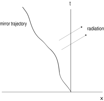
Figure 1: The worldline of a mirror moving to the left. The radiation emitted to the right is illustrated.

The trajectory for the mirror is

$$x=z(t),$$ (10)

where $|z^{\prime}(t)|<1$, and $z=0$ for $t\leq 0$. The boundary condition for the scalar field $\phi$ is

$$\phi(t,z(t))=0,$$ (11)

and the positive frequency mode function for $t>0$ is given by

$$\phi_{\omega}(x)=i(4\pi\omega)^{-1/2}[e^{-i\omega v}-e^{-i\omega(2\tau_{u}-u)}].$$ (12)

Here $u\equiv t-x$ and $v\equiv t+x$ are null coordinates, and the parameter $\tau_{u}$ is defined by

$$\tau_{u}-z(\tau_{u})=u.$$ (13)

The phase of the reflected wave is a function of $u$ only and is defined by

$$p(u)=2\tau_{u}-u.$$ (14)

The phase change of the out-going mode is due to the Doppler shift at the moving mirror. It is not surprising to see that the moving mirror can create particles, since the mirror boundary condition changes a positive frequency mode into a mixture of positive and negative frequencies.

The quantum field operator can be written as

$$\phi(x,t)=\int_{0}^{\infty}d\omega[a_{\omega}\phi_{\omega}+a_{\omega}^{\dagger}\phi_{\omega}^{*}],$$ (15)

where $a_{\omega}$ and $a_{\omega}^{\dagger}$ are annihilation and creation operators, respectively. The in-vacuum state $|0\rangle$ is defined by

$$\begin{array}[]{cc}a_{\omega}|0\rangle=0,&\forall\end{array}\omega.$$ (16)

We use the point-splitting method to extract out the Minkowski vacuum divergence. Let $\phi^{*}_{\omega}$ be replaced by $\phi^{*}_{\omega}(t+\epsilon,x)$, and

$$\langle\phi_{,\mu}\phi_{,\nu}\rangle=\lim_{\epsilon\rightarrow 0}\int_{0}^{\infty}\phi_{\omega,\mu}(r,t)\phi^{*}_{\omega,\nu}(r,t+\epsilon)d\omega.$$ (17)

The derivatives of the mode functions become

$$\phi_{\omega,t} = \left(\frac{\omega}{4\pi}\right)^{1/2}[e^{-i\omega v}-p^{\prime}(u)e^{-i\omega p(u)}],$$ (18)

$$\phi_{\omega,r} = \left(\frac{\omega}{4\pi}\right)^{1/2}[e^{-i\omega v}+p^{\prime}(u)e^{-i\omega p(u)}],$$ (19)

$$\phi_{\omega,t}^{*} = \left(\frac{\omega}{4\pi}\right)^{1/2}[e^{i\omega(v+\epsilon)}-p^{\prime}(u+\epsilon)e^{i\omega p(u+\epsilon)}],$$ (20)

and

$$\phi_{\omega,r}^{*}=\left(\frac{\omega}{4\pi}\right)^{1/2}[e^{i\omega(v+\epsilon)}+p^{\prime}(u+\epsilon)e^{i\omega p(u+\epsilon)}].$$ (21)

We insert these expressions into Eq. (17), and evaluate the $\omega$-integration using

$$\int_{0}^{\infty}e^{ibx}dx=\frac{i}{b},$$ (22)

and

$$\int_{0}^{\infty}\omega e^{ia\omega}d\omega=\frac{\partial}{i\partial a}\int_{0}^{\infty}e^{ia\omega}d\omega=-\frac{1}{a^{2}}.$$ (23)

Expanding the results in a power series in $\epsilon$ yields

$$\langle\phi_{,r}\phi_{,t}\rangle = -\frac{1}{4\pi}\left[\frac{1}{4}\left(\frac{p^{\prime\prime}}{p^{\prime}}\right)^{2}-\frac{1}{6}\frac{p^{\prime\prime\prime}}{p^{\prime}}\right]+O(\epsilon),$$ (24)

$$\langle\phi_{,t}\phi_{,r}\rangle = -\frac{1}{4\pi}\left[\frac{1}{4}\left(\frac{p^{\prime\prime}}{p^{\prime}}\right)^{2}-\frac{1}{6}\frac{p^{\prime\prime\prime}}{p^{\prime}}\right]+O(\epsilon),$$ (25)

$$\langle\phi_{,r}\phi_{,r}\rangle = -\frac{1}{4\pi}\left[\frac{2}{\epsilon^{2}}+\frac{2p^{\prime}}{(v-p(u))^{2}}-\frac{1}{4}\left(\frac{p^{\prime\prime}}{p^{\prime}}\right)^{2}+\frac{1}{6}\frac{p^{\prime\prime\prime}}{p^{\prime}}\right],$$ (26)

and

$$\langle\phi_{,t}\phi_{t}\rangle=-\frac{1}{4\pi}\left[\frac{2}{\epsilon^{2}}-\frac{2p^{\prime}}{(v-p(u))^{2}}-\frac{1}{4}\left(\frac{p^{\prime\prime}}{p^{\prime}}\right)^{2}+\frac{1}{6}\frac{p^{\prime\prime\prime}}{p^{\prime}}\right].$$ (27)

Here $\langle\phi_{,r}\phi_{,t}\rangle$ and $\langle\phi_{,t}\phi_{,r}\rangle$ are finite, and $\langle\phi_{,r}\phi_{,r}\rangle$and $\langle\phi_{,t}\phi_{,t}\rangle$ can be renormalized by discarding the $\epsilon^{-2}$ term. This term is independent of $p(u)$ (i.e. independent of trajectory) and can be recognized as the Minkowski vacuum divergence. The normal-ordered operator products are

$$\langle:\phi_{,r}\phi_{,t}:\rangle = \langle\phi_{,r}\phi_{,t}\rangle,$$ (28)

$$\langle:\phi_{,t}\phi_{,r}:\rangle = \langle\phi_{,t}\phi_{,r}\rangle,$$ (29)

$$\langle:\phi_{,r}\phi_{,r}:\rangle = \langle\phi_{,r}\phi_{,r}\rangle+\frac{1}{2\pi\epsilon^{2}},$$ (30)

and

$$\langle:\phi_{,t}\phi_{,t}:\rangle=\langle\phi_{,t}\phi_{,t}\rangle+\frac{1}{2\pi\epsilon^{2}}.$$ (31)

We next substitute the above relations into Eq. (8). The squared flux for an arbitrary trajectory becomes

$$\langle:T_{rt}^{2}:\rangle=\left(\frac{1}{4\pi}\right)^{2}\left[\frac{-4(p^{\prime})^{2}}{(v-p(u))^{4}}+\frac{3}{16}\left(\frac{p^{\prime\prime}}{p^{\prime}}\right)^{4}-\frac{1}{4}\frac{(p^{\prime\prime})^{2}p^{\prime\prime\prime}}{(p^{\prime})^{3}}+\frac{(p^{\prime\prime\prime})^{2}}{12(p^{\prime})^{2}}\right],$$ (32)

and the flux is

$$\langle T^{rt}\rangle=\frac{1}{4\pi}\left[\frac{1}{4}\left(\frac{p^{\prime\prime}}{p^{\prime}}\right)^{2}-\frac{1}{6}\frac{p^{\prime\prime\prime}}{p^{\prime}}\right].$$ (33)

3.2.1 A trajectory which produce a thermal spectrum of particles

Fulling and Davies [10, 11] have discussed a particular mirror trajectory which produces a steady thermal flux of particles at late times, and which models a two-dimensional evaporating black hole. Carlitz and Willey [9] have shown that the correlation function $C$ defined in Eq. (7) in this case is just that for a thermal state. The trajectory has the asymptotic form

$$\begin{array}[]{cc}z(t)\sim-t-Ae^{-2\kappa t+B},&t\rightarrow\infty,\end{array}$$ (34)

where $A,B,$ and $\kappa$ are positive constants. Here

$$p(u)=2\tau_{u}-u\sim B-A^{-\kappa(u+B)},\quad u\rightarrow\infty.$$ (35)

Substituting this form Eq. (32) gives the normal-ordered squared flux

$$\langle:T_{rt}^{2}(x):\rangle=\left(\frac{1}{4\pi}\right)^{2}\left[\frac{\kappa^{4}}{48}-\frac{16A^{2}\kappa^{2}e^{-2\kappa(u+B)}}{(v-B+Ae^{-\kappa(u+B)})^{4}}\right]\to\left(\frac{1}{4\pi}\right)^{2}\frac{\kappa^{4}}{48},\quad u\to\infty.$$ (36)

Similarly, the expectation value of the flux is

$$\langle:T^{rt}(x):\rangle=-\langle:T_{rt}(x):\rangle=\frac{\kappa^{2}}{48\pi}.$$ (37)

The squared flux is related to the mean flux by

$$\langle:T_{rt}^{2}(x):\rangle=3\langle:T_{rt}:\rangle^{2},$$ (38)

and the relative deviation is

$$\frac{\langle:\triangle T_{rt}:\rangle}{\langle:T_{rt}:\rangle}=\frac{\sqrt{\langle:T_{rt}^{2}(x):\rangle-\langle:T_{rt}:\rangle^{2}}}{\langle:T_{rt}:\rangle}=\sqrt{2}.$$ (39)

The fractional flux fluctuations are thus of order unity.

Correlation function

The function $\langle T_{rt}(x)T_{rt}(x^{\prime})\rangle$ is finite except in the short distance limit $x^{\prime}-x\rightarrow 0$. On the other hand, the normal-ordered function $\langle:T_{rt}(x)T_{rt}(x^{\prime}):\rangle$ has a finite value in this limit. Here we restrict our discussion to the latter function. We define a normalized correlation function as (note that this is distinct from the function $C$ defined in Eq. (7) )

$$\xi(\triangle t)=\frac{\langle:T_{rt}(t)T_{rt}(t^{\prime}):\rangle-\langle:T_{rt}(t):\rangle\langle:T_{rt}(t^{\prime}):\rangle}{\langle:T_{rt}(t):\rangle\langle:T_{rt}(t^{\prime}):\rangle},$$ (40)

where $\triangle t=|t-t^{\prime}|$ and the spatial points are coincident. For the specific trajectory of Eq. (34), $\xi(\triangle t)$ is

$$\xi(\triangle t)=288\left[\frac{e^{-\kappa\triangle t}}{(1-e^{-\kappa\triangle t})^{2}}-\frac{1}{(\kappa\triangle t)^{2}}\right]^{2},$$ (41)

which is plotted in Fig. $2$. Note that $\xi(\triangle t)$ is finite for all $\triangle t\geq 0$.

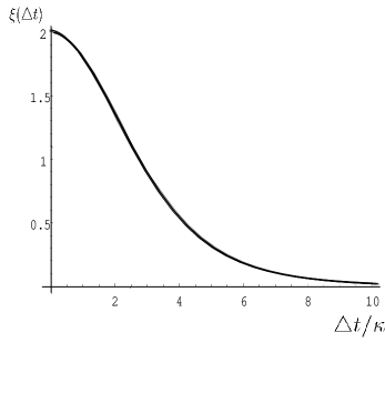
Figure 2: The correlation function for thermal radiation in two dimensional spacetime.

$$\xi(\tau_{c})=\frac{1}{2}\xi(0),$$ (42)

and is approximately

$$\tau_{c}\approx\frac{3}{\kappa}.$$ (43)

3.3 Two dimensional black hole

Fulling and Davies have shown that the mirror trajectory of Eq. (34) produces the same quantum state in the asymptotic region as does a two dimensional evaporating black hole of mass $M$ if $\kappa=1/4M$. Thus the flux and squared flux for the 2-D black hole are

$$\langle:T^{rt}(x):\rangle=\frac{1}{768\pi M^{2}},$$ (44)

and

$$\langle:T_{rt}^{2}(x):\rangle=3\langle:T_{rt}(x):\rangle^{2}.$$ (45)

The correlation time $\tau_{c}$ becomes

$$\tau_{c}=11M.$$ (46)

Thus the Hawking flux undergoes large fluctuations, varying by a factor of order unity on a time scale of order $11M$.

3.4 Four dimensional black hole

In four dimensions, the treatment of black hole evaporation becomes more complicated than in two dimensions. This is due to the angular degrees of freedom and the resultant potential barrier around the black hole. Ingoing and outgoing waves experience scattering off of this potential barrier. We will consider the case of a nonrotating, uncharged (Schwarzschild) black hole, and will follow the treatment of DeWitt [12]. The mode functions are of the form

$$u=\frac{1}{2\pi r\sqrt{2\omega}}R_{l}(\omega|r)Y_{lm}(\theta,\phi)\,e^{-i\omega t},$$ (47)

where the $Y_{lm}(\theta,\phi)$ are the usual spherical harmonics. Vector signs will be used to indicate the two independent modes which have the asymptotic forms

$$\overrightarrow{R}_{l}(\omega|r)\to\left\{\begin{array}[]{cc}e^{i\omega r^{*}}+\overrightarrow{A}_{l}(\omega)e^{i\omega r*}&,r^{*}\to-\infty\\ B_{l}(\omega)e^{i\omega r^{*}}&,r^{*}\to\infty\end{array}\right.$$ (48)

and

$$\overleftarrow{R}_{l}(\omega|r)\to\left\{\begin{array}[]{cc}B_{l}(\omega)e^{-i\omega r^{*}}&,r^{*}\to-\infty\\ e^{-i\omega r^{*}}+\overleftarrow{A}_{l}(\omega)e^{i\omega r^{*}}&r^{*}\to\infty\end{array}\right.,$$ (49)

where $r^{*}$ is the usual tortoise coordinate

$$r^{*}=r+2M\ln\left(\frac{r}{2M}-1\right).$$ (50)

The transmission coefficients $B_{l}$ and reflection coefficients $A_{l}$ satisfy the relations

$$|\overleftarrow{A_{l}}(\omega)|=|\overrightarrow{A_{l}}(\omega)|,$$ (51)

$$1-|\overrightarrow{A_{l}}(\omega)|^{2}=1-|\overleftarrow{A_{l}}(\omega)|^{2}=|B_{l}(\omega)|^{2},$$ (52)

and

$$\overrightarrow{A_{l}}^{*}(\omega)B_{l}(\omega)=-B^{*}_{l}\overleftarrow{A_{l}}(\omega).$$ (53)

The components of the energy-momentum tensor in the Unruh vacuum state near future null infinity are of the form (See Ref. 12 for details.)

$$\langle\phi_{,\mu}\phi_{,\nu}\rangle\sim\sum_{l,m}\int_{0}^{\infty}[\overleftarrow{u}_{,\mu}\overleftarrow{u}_{,\nu}^{*}+\coth(4\pi M\omega)\overrightarrow{u}_{,\mu}\overrightarrow{u}_{,\nu}^{*}]d\omega.$$ (54)

The asymptotic form of the mode functions are

$$\overrightarrow{u}=\frac{1}{2\pi r\sqrt{2\omega}}B_{l}(\omega)e^{i\omega r^{*}}Y_{lm}\,e^{-i\omega t},$$ (55)

and

$$\overleftarrow{u}=\frac{1}{2\pi r\sqrt{2\omega}}Y_{lm}e^{-i\omega t}(e^{-i\omega r^{*}}+\overleftarrow{A}_{l}(\omega)e^{i\omega r^{*}}).$$ (56)

The derivatives of these mode functions become

$$\overleftarrow{u}_{,r}\overleftarrow{u}^{*}_{,t} = \frac{\omega|Y_{lm}|^{2}}{8\pi^{2}r^{2}}(1-|\overleftarrow{A_{l}}|^{2}+\overleftarrow{A_{l}}^{*}e^{-2i\omega r}-\overleftarrow{A_{l}}e^{2i\omega r}),$$ (57)

$$\overleftarrow{u}_{,t}\overleftarrow{u}^{*}_{,r} = \frac{\omega|Y_{lm}|^{2}}{8\pi^{2}r^{2}}(1-|\overleftarrow{A_{l}}|^{2}-\overleftarrow{A_{l}}^{*}e^{-2i\omega r}+\overleftarrow{A_{l}}e^{2i\omega r}),$$ (58)

$$\overleftarrow{u}_{,t}\overleftarrow{u}^{*}_{,t} = \frac{\omega|Y_{lm}|^{2}}{8\pi^{2}r^{2}}(1+|\overleftarrow{A_{l}}|^{2}+\overleftarrow{A_{l}}^{*}e^{-2i\omega r}+\overleftarrow{A_{l}}e^{2i\omega r}),$$ (59)

$$\overleftarrow{u}_{,r}\overleftarrow{u}^{*}_{,r} = \frac{\omega|Y_{lm}|^{2}}{8\pi^{2}r^{2}}(1+|\overleftarrow{A_{l}}|^{2}+\overleftarrow{A_{l}}^{*}e^{-2i\omega r}+\overleftarrow{A_{l}}e^{2i\omega r}),$$ (60)

$$\overrightarrow{u}_{,r}\overrightarrow{u}^{*}_{,t} = \frac{-\omega|B_{l}|^{2}|Y_{lm}|^{2}}{8\pi^{2}r^{2}},$$ (61)

$$\overrightarrow{u}_{,t}\overrightarrow{u}^{*}_{,r} = \frac{-\omega|B_{l}|^{2}|Y_{lm}|^{2}}{8\pi^{2}r^{2}},$$ (62)

$$\overrightarrow{u}_{,r}\overrightarrow{u}^{*}_{,r} = \frac{\omega|B_{l}|^{2}|Y_{lm}|^{2}}{8\pi^{2}r^{2}},$$ (63)

and

$$\overrightarrow{u}_{,t}\overrightarrow{u}^{*}_{,t}=\frac{\omega|B_{l}|^{2}|Y_{lm}|^{2}}{8\pi^{2}r^{2}}.$$ (64)

Substitution of these relation into Eq. (54) and use of the summation formula

$$\sum_{m}|Y_{lm}|^{2}=\frac{2l+1}{4\pi},$$ (65)

yields

$$\langle\phi_{,r}\phi_{,t}\rangle = \sum_{l,m}\int_{0}^{\infty}[\overleftarrow{u}_{,r}\overleftarrow{u}_{,t}^{*}+\coth(4\pi M\omega)\overrightarrow{u}_{,r}\overrightarrow{u}_{,t}^{*}]d\omega$$ (66)

$$= \frac{-\sin\theta}{4\pi^{2}}\sum_{l,m}|Y_{lm}|^{2}\int_{0}^{\infty}\frac{|B_{l}|^{2}\omega}{e^{8\pi M\omega}-1}d\omega$$

$$+\frac{\sin\theta}{32\pi^{3}}\sum_{l}(2l+1)\int_{0}^{\infty}\omega(\overleftarrow{A_{l}}^{*}e^{-2i\omega r}-\overleftarrow{A_{l}}e^{2i\omega r})d\omega.$$

The first term on the right hand side is $\langle T_{rt}\rangle$. Similar calculations give us these derivatives in terms of the mean flux $\langle T^{rt}\rangle$ as

$$\langle\phi_{,r}\phi_{,t}\rangle = -\langle T^{rt}\rangle+I_{2,}$$ (67)

$$\langle\phi_{,t}\phi_{,r}\rangle = -\langle T^{tr}\rangle-I_{2,}$$ (68)

$$\langle\phi_{,r}\phi_{,r}\rangle = \langle T^{rt}\rangle+I_{0}-I_{1,}$$ (69)

and

$$\langle\phi_{,t}\phi_{,t}\rangle=\langle T^{rt}\rangle+I_{0}+I_{1}.$$ (70)

where the integrals $I_{0},$ $I_{1}$ and $I_{2}$ are

$$I_{0}=\frac{\sin\theta}{16\pi^{3}}\sum_{l}(2l+1)\int^{\infty}_{0}\omega d\omega,$$ (71)

$$I_{1}=\frac{\sin\theta}{16\pi^{3}}\sum_{l}(2l+1)\int^{\infty}_{0}\omega A(\omega)\cos(\delta(\omega)+2r\omega)d\omega,$$ (72)

and

$$I_{2}=-i\frac{\sin\theta}{16\pi^{3}}\sum_{l}(2l+1)\int^{\infty}_{0}\omega A(\omega)\sin(\delta(\omega)+2r\omega)d\omega.$$ (73)

We can identity $I_{0}$ as the Minkowski divergence, and symmetrization removes the pure imaginary term $I_{2}$. Discarding these two terms yields

$$\frac{1}{2}(\langle:\phi_{,r}\phi_{,t}:\rangle+\langle:\phi_{,t}\phi_{,r}:\rangle) = \langle:T_{rt}:\rangle=\langle:T_{tr}:\rangle,$$ (74)

$$\langle:\phi_{,r}\phi_{,r}:\rangle = -\langle:T_{rt}:\rangle-I_{1,}$$ (75)

and

$$\langle:\phi_{,t}\phi_{,t}:\rangle=-\langle:T_{rt}:\rangle+I_{1.}$$ (76)

Using the relations

$$\begin{array}[]{cc}A(\omega)\to A_{0,}&\omega\to 0,\\ A(\omega)\to 0,&\omega\to\infty,\end{array}$$

and

$$\begin{array}[]{cc}\delta(\omega)\to\delta_{0},&\omega\to\infty,\end{array}$$

the integral $I_{1}$ at large distance, $r\to\infty$, becomes

$$\int^{\infty}_{0}\omega A(\omega)\cos(\delta(\omega)+2r\omega)d\omega = \frac{1}{r^{2}}\int^{\infty}_{0}xA\left(\frac{x}{r}\right)\cos\left[\delta\left(\frac{x}{r}\right)+2x\right]d\omega$$

$$\sim \frac{A_{0}}{r^{2}}\int^{\infty}_{0}\cos(2x+\delta_{0})xdx\propto\frac{1}{r^{2}}.$$

Thus the term $I_{1}$ is much smaller than the mean flux

$$\langle T^{rt}\rangle=\frac{\sin\theta}{16\pi^{3}}\sum_{l}(2l+1)\int^{\infty}_{0}\frac{|B_{l}|^{2}}{e^{8\pi M\omega-1}}d\omega$$ (78)

which is a nonzero constant at large distance, and hence $I_{1}$ can be ignored. The squared flux becomes

$$\langle:T_{rt}^{2}:\rangle = \langle:T_{rt}:\rangle^{2}+\langle:\phi_{,r}\phi_{,t}:\rangle\langle:\phi_{,t}\phi_{,r}:\rangle+\langle:\phi_{,r}\phi_{,r}:\rangle\langle:\phi_{,t}\phi_{,t}:\rangle$$ (79)

$$= 2\langle:T_{rt}:\rangle^{2}+(\langle:T_{rt}:\rangle-I_{1})(\langle:T_{rt}:\rangle+I_{1})$$

$$\approx 3\langle T_{rt}\rangle^{2}.$$

We thus get the same relation between the squared flux and the mean flux as in the case of a two dimensional evaporating black hole.

Next we will discuss the normal-ordered correlation function and ignore the contribution from $I_{1}$. From Eq. (54), we have

$$\langle:\phi_{,r}(x)\phi_{,r}(x^{\prime}):\rangle = Re\left[\frac{1}{16\pi^{2}r^{2}}\sum_{l}(2l+1)\int_{0}^{\infty}\frac{|B_{l}|^{2}\omega e^{i\omega\triangle t}}{e^{8\pi M\omega}-1}d\omega\right],$$ (80)

$$\langle:\phi_{,t}(x)\phi_{,t}(x^{\prime}):\rangle = Re\left[\frac{1}{16\pi^{2}r^{2}}\sum_{l}(2l+1)\int_{0}^{\infty}\frac{|B_{l}|^{2}\omega e^{i\omega\triangle t}}{e^{8\pi M\omega}-1}d\omega\right],$$ (81)

$$\langle:\phi_{,r}(x)\phi_{,t}(x^{\prime}):\rangle = Re\left[-\frac{1}{16\pi^{2}r^{2}}\sum_{l}(2l+1)\int_{0}^{\infty}\frac{|B_{l}|^{2}\omega e^{i\omega\triangle t}}{e^{8\pi M\omega}-1}d\omega\right],$$ (82)

and

$$\langle:\phi_{,t}(x)\phi_{,r}(x^{\prime}):\rangle=Re\left[-\frac{1}{16\pi^{2}r^{2}}\sum_{l}(2l+1)\int_{0}^{\infty}\frac{|B_{l}|^{2}\omega e^{i\omega\triangle t}}{e^{8\pi M\omega}-1}d\omega\right],$$ (83)

where $\triangle t=t^{\prime}-t$. The correlation function defined in Eq. (40) now becomes

$$\xi(\triangle t)=\frac{2\left(Re\left[\sum_{l}(2l+1)\int_{0}^{\infty}\frac{|B_{l}|^{2}\omega e^{i\omega\triangle t}}{e^{8\pi M\omega}-1}d\omega\right]\right)^{2}}{\left(Re\left[\sum_{l}(2l+1)\int_{0}^{\infty}\frac{|B_{l}|^{2}\omega}{e^{8\pi M\omega}-1}d\omega\right]\right)^{2}}.$$ (84)

For our purposes, the transmission coefficient may be approximated by a step function

$$B_{l}(p)\approx\Theta(\sqrt{27}M\omega-l).$$ (85)

In this approximation, modes with energies below the peak of the angular momentum barrier are assumed to be perfectly reflected, and those with energies above the peak are completely transmitted. This is a reasonably good approximation, as may be seen by examining Figure 1 in Ref. [13], where numerical results for the transmission and reflection coefficients are given. The summation on $l$ yields

$$\sum_{l}(2l+1)|B_{l}|^{2}=\sum_{l}(2l+1)\Theta(\sqrt{27}M\omega-l)=27M^{2}\omega^{2}+6\sqrt{3}M\omega+1\,,$$ (86)

and the numerator of Eq. (84) becomes

$$S(\triangle t) = Re\left(\sum_{l}(2l+1)\int_{0}^{\infty}\frac{|B_{l}|^{2}\omega e^{i\omega\triangle t}}{e^{8\pi M\omega}-1}d\omega\right)$$ (87)

$$= Re\left(\int_{0}^{\infty}\frac{(27M^{2}\omega^{2}+6\sqrt{3}M\omega+1)\omega e^{ip\triangle t}}{e^{8\pi M\omega}-1}d\omega\right)$$

$$= \frac{27}{(8\pi)^{4}M^{2}}Re\left(\int_{0}^{\infty}\frac{x^{3}e^{ibx}}{e^{x}-1}dx\right)+\frac{6\sqrt{3}}{(8\pi)^{3}M^{2}}Re\left(\int_{0}^{\infty}\frac{x^{2}e^{ibx}}{e^{x}-1}dx\right)$$

$$+\frac{1}{(8\pi)^{2}M^{2}}Re\left(\int_{0}^{\infty}\frac{xe^{ibx}}{e^{x}-1}dx\right),$$

where $x=8\pi M\omega$ and $b=\triangle t/8\pi M$. The correlation function is

$$\xi(\triangle t)=\frac{2S(\triangle t)^{2}}{S(0)^{2}},$$ (88)

and is plotted in Fig. $3$.

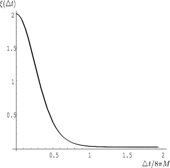
Figure 3: The correlation function for the radiation from a black hole in four dimensional spacetime.

The correlation time $\tau_{c}$ is around $0.3(8\pi M)\approx 8M$ . As in the two dimensional case, the four dimensional Hawking radiation undergoes large flux fluctuations on a time scale of about $8M$.

3.5 Flux Fluctuations as Thermal Fluctuations

It is reasonable to expect that the flux fluctuations computed in the previous subsection can be interpreted as ordinary thermal fluctuations. Thermal fluctuations of the energy in the canonical ensemble are described by the relation

$$\frac{\Delta E}{E}=\frac{T\,\sqrt{k_{B}C_{V}}}{E}\,,$$ (89)

where $E$ is the mean energy at temperature $T$ for a system with heat capacity $C_{V}$. In the case of thermal radiation, $E\propto T^{4}$, so $C_{V}=4E/T$, and hence

$$\frac{\Delta E}{E}=2\sqrt{\frac{k_{B}T}{E}}\,.$$ (90)

Note that $E/(k_{B}T)$ is a measure of the mean number of photons in the thermal radiation, so the above result is the familiar $1/\sqrt{N}$ statistical fluctuation.

Let us take $E$ to be the energy emitted by a black hole in one correlation time, $\tau_{c}\approx 8M$, and the power emitted to be that calculated by Page [14] for photon emission from a Schwarzscild black hole:

$$P=3.4\times 10^{-5}\,M^{-2}\,.$$ (91)

This leads to a rather small number of photons emitted per correlation time,

$$\frac{E}{k_{B}T}\approx 8\times 10^{-3}$$ (92)

and rather large fractional energy fluctuations

$$\frac{\Delta E}{E}\approx 23\,.$$ (93)

This estimate is somewhat larger than the result obtained from the normal ordered squared flux in the previous subsection. However, it is a very rough estimate which depends upon our choice for the energy $E$ and the collecting time. If we had chosen to integrate the flux for a time longer than $\tau_{c}$, the statistical fluctuations would be somewhat reduced. Also, the spectrum of particles emitted by a black hole is not exactly Planckian, but has been filtered by the angular momentum barrier.

4 The Physics of the Cross Term

We now turn to examining the cross term between the vacuum fluctuations and the finite, state dependent parts. Recall that this contribution is singular in the coincidence limit, and hence does not lead to a well defined local definition of the squared flux. If it is not to be subtracted by some renormalization method, then it can only be given physical meaning by dealing with time or space averages.

4.1 Switching Functions

One possibility is to suppose that we operationally measure the flux with a model detector which has a finite response time. Suppose that the response of our detector is described by a Lorentzian function with characteristic width $\tau$,

$$f(t)=\frac{\tau}{\pi}\frac{1}{(t-t_{0})^{2}+\tau^{2}}.$$ (94)

The averaged squared flux becomes

$$\langle T_{rt}^{2}(x)\rangle_{average}=\int_{-\infty}^{\infty}\int_{-\infty}^{\infty}f(t)f(t^{\prime})\langle T_{rt}(x)T_{rt}(x^{\prime})\rangle dtdt^{\prime}.$$ (95)

We will examine the case of the thermal flux from a mirror or black hole in two dimensions, and assume that the sampling time is short compared to the correlation time, $\tau\ll\tau_{c}$. In this case, the correlation functions are approximately constant, and the average of the normal ordered term is

$$A_{2}=\int_{-\infty}^{\infty}\int_{-\infty}^{\infty}f(t)f(t^{\prime})\langle:T_{rt}(x)T_{rt}(x^{\prime}):\rangle dtdt^{\prime}\approx\langle:T_{rt}(x)T_{rt}(x^{\prime}):\rangle.$$ (96)

The average of the cross term can be written as

$$A_{1} =\int_{-\infty}^{\infty}\int_{-\infty}^{\infty}f(t)f(t^{\prime})\left[\langle:\phi(x)_{,r}\phi(x^{\prime})_{,r^{\prime}}:\rangle\langle\phi(x)_{,t}\phi(x^{\prime})_{,t^{\prime}}\rangle_{M}+\right.$$ (97)

$$\left.\langle:\phi(x)_{,t}\phi(x^{\prime})_{,t^{\prime}}:\rangle\langle\phi(x)_{,r}\phi(x^{\prime})_{,r^{\prime}}\rangle_{M}\right]dtdt^{\prime}\approx 2\langle:T^{rt}:\rangle\int_{-\infty}^{\infty}f(t)f(t^{\prime})\frac{1}{-2\pi(t-t^{\prime})^{2}}dtdt^{\prime}$$

$$\approx \frac{1}{4\pi\tau^{2}}\,\langle T^{rt}\rangle,$$

where we have used Eq. (B8) in Appendix B.

For comparison, it is of interest to give the average of the vacuum term

$$A_{0} =\int_{-\infty}^{\infty}\int_{-\infty}^{\infty}f(t)f(t^{\prime})\langle\phi(x)_{,r}\phi(x^{\prime})_{,r^{\prime}}\rangle_{M}\langle\phi(x)_{,t}\phi(x^{\prime})_{,t^{\prime}}\rangle_{M}dtdt^{\prime}$$ (98)

$$= \int_{-\infty}^{\infty}\int_{-\infty}^{\infty}f(t)f(t^{\prime})\frac{1}{4\pi^{2}(t-t^{\prime})^{4}}dtdt^{\prime}=\frac{1}{64\pi^{2}\tau^{4}}\,,$$

using Eq. (B16).

In the case of a two-dimensional black hole, where $\langle T^{rt}\rangle=1/(768\pi M^{2})$ and $\langle:T_{rt}^{2}:\rangle=3\langle T_{rt}\rangle^{2}$, we see that $A_{0}\gg A_{1}\gg A_{2}$ when $T\gg M$. If we were to let $T\approx M$, our assumption that the correlation functions are constant would no longer be exact. Nonetheless, this calculation should give a resonable order of magnitude estimate, and predicts that all three terms are of the same order of magnitude.

4.2 A Mirror as a Flux Detector

Here we will examine a model in which the flux is measured by the force which it exerts on a reflecting or absorbing surface. All of our discussion will be in one spatial dimension, so the force on a partially reflecting surface is

$$F=r\,:T^{rt}:\,,$$ (99)

where $0<r\leq 2$ and $\frac{1}{2}r$ is the fraction of the radiation which is reflected. Consider a mirror with mass $m$ which starts at rest at time $t=0$ . The mean velocity and mean squared velocity at $t=\tau$ are

$$\langle v\rangle=\frac{1}{m}\int_{0}^{\tau}\langle F\rangle dt$$ (100)

and

$$\langle v^{2}\rangle=\frac{1}{m^{2}}\int_{0}^{\tau}\int_{0}^{\tau}\langle F(t)F(t^{\prime})\rangle dtdt^{\prime}.$$ (101)

The force two-point function is

$$\langle F(t)F(t^{\prime})\rangle = r^{2}\langle:T_{rt}(t)::T_{rt}(t^{\prime}):\rangle$$

$$= r^{2}\langle:T_{rt}(t)T_{rt}(t^{\prime}):\rangle+r^{2}\langle T_{rt}T_{rt}\rangle_{cross}+r^{2}\langle T_{rt}T_{rt}\rangle_{M}.$$

We are interested in the difference between the fluctuations in a given state and those in the Minkowski vacuum, and so drop the vacuum term. We then define the fluctuations by subtracting out the square of the mean value:

$$\langle\triangle T^{2}\rangle=\langle T^{2}\rangle-\langle T\rangle^{2}.$$ (103)

The normal-ordered flux fluctuation is given by

$$\langle\triangle T_{rt}^{2}\rangle_{NO} = \langle:T_{rt}(t)T_{rt}(t^{\prime}):\rangle-\langle T_{rt}(t)\rangle\langle T_{rt}(t^{\prime})\rangle$$

$$= \langle:\phi_{,r}(t)\phi_{,r}(t^{\prime}):\rangle\langle:\phi_{,t}(t)\phi_{,t}(t^{\prime}):\rangle+\langle:\phi_{,r}(t)\phi_{,t}(t^{\prime}):\rangle\langle:\phi_{,t}(t)\phi_{,r}(t^{\prime}):\rangle,$$

and the cross-term contribution is

$$\langle\triangle T_{rt}^{2}\rangle_{cross}=\langle:\phi_{,r}(t)\phi_{,r}(t^{\prime}):\rangle\langle\phi_{,t}(t)\phi_{,t}(t^{\prime})\rangle_{M}+\langle:\phi_{,t}(t)\phi_{,t}(t^{\prime}):\rangle\langle\phi_{,r}(t)\phi_{,r}(t^{\prime})\rangle_{M.}$$ (105)

The velocity fluctuation can be written as

$$\langle\triangle v^{2}\rangle = \langle v^{2}\rangle-\langle v\rangle^{2}$$ (106)

$$= \langle\triangle v^{2}\rangle_{NO}+\langle v^{2}\rangle_{cross}$$

$$= \frac{r^{2}}{m^{2}}\int\langle\triangle T_{rt}^{2}\rangle_{NO}dtdt^{\prime}+\frac{r^{2}}{m^{2}}\int\langle\triangle T_{rt}^{2}\rangle_{cross}dtdt^{\prime}.$$

4.2.1 Coherent state

A coherent state describes a classical field excitation and is hence a useful model to reveal the effects of the cross term. Consider a single-mode coherent state $|z\rangle$ for a mode with frequency $\omega_{0}$

$$a_{\omega}|z\rangle=\delta_{\omega\omega_{0}}z|z\rangle.$$ (107)

The free quantum field expanded in normal modes is

$$\phi(x,t)=\sum_{\omega}(a_{\omega}\phi_{\omega}+a_{\omega}^{\dagger}\phi_{\omega}^{*}),$$ (108)

where the mode function for a standing wave in a box of length $L$ is

$$\phi_{\omega}=\frac{1}{\sqrt{2\omega L}}e^{-i\omega t}\sin(\omega x).$$ (109)

Assume that the mirror remains approximately stationary, as will be the case when its mass is large, and set $x=x^{\prime}$. Further, let $z=Re^{i\triangle}$ and find

$$\langle z|:\phi_{,r}(x)\phi_{,r^{\prime}}(x^{\prime}):|z\rangle=\frac{\omega_{0}|z|^{2}\cos^{2}(\omega_{0}r)}{L}[\cos(\omega_{0}(t-t^{\prime}))+\cos(2\triangle-\omega_{0}(t+t^{\prime}))],$$ (110)

and

$$\langle z|:\phi_{,t}(x)\phi_{,t^{\prime}}(x^{\prime}):|z\rangle=\frac{\omega_{0}|z|^{2}\sin^{2}(\omega_{0}r)}{L}[\cos(\omega_{0}(t-t^{\prime}))-\cos(2\triangle-2\omega_{0}t+\omega_{0}(t+t^{\prime}))].$$ (111)

We also have that

$$\langle\phi(x)_{,t}\phi(x^{\prime})_{,t^{\prime}}\rangle_{M}=\langle\phi(x)_{,r}\phi(x^{\prime})_{,r^{\prime}}\rangle_{M}=-\frac{1}{2\pi(t-t^{\prime})^{2}}.$$ (112)

For the coherent state, the only fluctuations come from the cross term because

$$\langle z|:T_{\mu\nu}T_{\rho\sigma}:|z\rangle=\langle z|:T_{\mu\nu}:|z\rangle\langle z|:T_{\rho\sigma}:|z\rangle.$$ (113)

The velocity fluctuation is then

$$\langle\triangle v^{2}\rangle = \frac{r^{2}}{m^{2}}\int\langle\triangle T_{rt}^{2}\rangle_{cross}dtdt^{\prime}$$

$$= \frac{-\omega_{0}|z|^{2}r^{2}}{\pi Lm^{2}}\int\{\cos^{2}(\omega_{0}r)[\cos(\omega_{0}(t-t^{\prime}))+\cos(2\triangle-\omega_{0}(t+t^{\prime}))]$$

$$+\sin^{2}(\omega_{0}r)[\cos(\omega_{0}(t-t^{\prime}))-\cos(2\triangle-2\omega_{0}t+\omega_{0}(t+t^{\prime}))]\}\frac{1}{(t-t^{\prime})^{2}}dtdt^{\prime}.$$

This integral is poorly defined due to the singularity of the integrand at $t=t^{\prime}$. A possible resolution of this difficulty is to employ a trick which has been used by various authors under the rubrics of “generalized principle value” [15] or “differential regularization” [16]. In any case, it involves writing the singular factor as a derivative of a less singular function, and then integrating by parts. We will also assume that the flux is adiabatically switched on in the past and off again in the future, so that any surface terms vanish. Thus we may use relations such as

$$\int f(t,t^{\prime})\frac{1}{(t-t^{\prime})^{2}}dtdt^{\prime}=\frac{1}{2}\int[\partial_{t}\partial_{t^{\prime}}f(t,t^{\prime})]\,\ln((t-t^{\prime})^{2})dtdt^{\prime}\,.$$ (115)

Let $r=0$ , $x=\omega_{0}t$, and $x^{\prime}=\omega_{0}t^{\prime}$. The velocity fluctuation becomes

$$\langle\triangle v^{2}\rangle=-\frac{r^{2}\omega_{0}^{3}|z|^{2}}{2\pi Lm^{2}}\int_{0}^{\tau}\int_{0}^{\tau}[\cos(\omega_{0}t-\omega_{0}t^{\prime})+\cos(2\triangle-\omega_{0}t-\omega_{0}t^{\prime})]\ln[\omega_{0}(t-t^{\prime})]^{2}dtdt^{\prime}$$ (116)

The integral may now be written in terms of the variables $U=x-x^{\prime}$ and $V=x+x^{\prime}$, using the identity

$$\int_{0}^{\tau}\int_{0}^{\tau}dtdt^{\prime}=\frac{1}{2}\left(\int_{-\tau}^{0}dU\int_{-U}^{U+2\tau}dV+\int_{0}^{\tau}dU\int_{U}^{2\tau-U}dV\right),$$ (117)

and evaluated in terms of sine and cosine integral functions. We are primarily interested in the asymptotic form for large $\tau$, which is

$$\langle\triangle v^{2}\rangle\sim\frac{2r^{2}\omega_{0}^{2}|z|^{2}}{3Lm^{2}}\,\tau\,.$$ (118)

This result shows that the cross term leads to a contribution to the mean squared velocity of the mirror which grows linearly in time. This is the characteristic time dependence of a random walk process. It is useful to compare the fluctuations with the mean velocity

$$\langle v\rangle = \frac{r}{m}\int_{0}^{\tau}\langle T^{rt}\rangle dt$$ (119)

$$= \frac{|z|^{2}\,r}{4Lm}\sin(2\omega_{0}x)[\cos(2\triangle)-\cos(2\triangle-2\omega_{0}\tau)].$$

The mean velocity happens to vanish at the special point $x=0$ at which we evaluated $\langle\triangle v^{2}\rangle$. However, at a more general point it is of order

$$\langle:v:\rangle\approx\frac{|z|^{2}\,r}{Lm},$$ (120)

and the fractional velocity fluctuations becomes of order

$$\frac{\sqrt{\langle\triangle v^{2}\rangle}}{\langle v\rangle}\approx\frac{\omega_{0}\sqrt{L\tau}}{|z|}.$$ (121)

Although this quantity grows in time, it is also inversely proportional to the amplitude $|z|$. Thus for a nearly classical state ($|z|\gg 1$), it can remain small for a very long time.

4.2.2 Thermal state created by moving mirror

Consider the 2-D moving mirror with an arbitrary trajectory. These flux fluctuation, without the vacuum term, can be written as

$$\langle\triangle T_{rt}^{2}\rangle_{total}=\langle\triangle T_{rt}^{2}\rangle_{no}+\langle\triangle T_{rt}^{2}\rangle_{cross}$$ (122)

$$= 2\left(\frac{1}{4\pi}\right)^{2}\left[\frac{p^{\prime}(u)p^{\prime}(u^{\prime})}{(p(u)-p(u^{\prime}))^{2}}-(\frac{p^{\prime}(u^{\prime})}{(v-p(u^{\prime}))^{2}})^{2}-(\frac{p^{\prime}(u)}{(v-p(u))^{2}})^{2}-\frac{1}{(t-t^{\prime})^{4}}\right],$$

where

$$\langle\triangle T_{rt}^{2}\rangle_{no} = 2\left(\frac{1}{4\pi}\right)^{2}\left[-(\frac{p^{\prime}(u^{\prime})}{(v-p(u^{\prime}))^{2}})^{2}-(\frac{p^{\prime}(u)}{(v-p(u))^{2}})^{2}+(\frac{p^{\prime}(u)p^{\prime}(u^{\prime})}{(p(u)-p(u^{\prime}))^{2}})^{2}+\frac{1}{(t-t^{\prime})^{4}}\right.$$ (123)

$$\left.-\frac{2p^{\prime}(u)p^{\prime}(u^{\prime})}{(p(u)-p(u^{\prime}))^{2}(t-t^{\prime})^{2}}\right],$$

and

$$\langle\triangle T_{rt}^{2}\rangle_{cross}=4\left(\frac{1}{4\pi}\right)^{2}\left[\frac{p^{\prime}(u)p^{\prime}(u^{\prime})}{(p(u)-p(u^{\prime}))^{2}}-\frac{1}{(t-t^{\prime})^{2}}\right]\frac{1}{(t-t^{\prime})^{2}}.$$ (124)

The total velocity fluctuation is

$$\langle\triangle v^{2}\rangle_{total} = \frac{r^{2}}{m^{2}}\int_{0}^{\tau}\int_{0}^{\tau}\langle\triangle T_{rt}^{2}\rangle_{total}dtdt^{\prime}$$ (125)

$$= \frac{2\,r^{2}}{(4\pi)^{2}m^{2}}\int_{0}^{\tau}\int_{0}^{\tau}\left\{\left[\frac{p^{\prime}(u)p^{\prime}(u^{\prime})}{(p(u)-p(u^{\prime}))^{2}}\right]^{2}\right.$$

$$- \left.\left[\frac{p^{\prime}(u)}{(v^{\prime}-p(u))^{2}}\right]^{2}-\left[\frac{p^{\prime}(u^{\prime})}{(v-p(u^{\prime}))^{2}}\right]^{2}-\frac{1}{(t-t^{\prime})^{4}}\right\}dtdt^{\prime}.$$

As before, we suppose that $\langle\triangle T_{rt}^{2}\rangle_{total}$ is multiplied by a swithching function which vanishes in the past and in the future. Then the $(t-t^{\prime})^{-4}$ term gives no contribution after an integration by parts. Note that this term is of the same form as the pure vacuum contribution, so our results will not depend upon whether the vacuum part was subtracted beforehand or not.

Consider the trajectory which produces a thermal spectrum, $p(u)=B-Ae^{-\kappa(u+B)}$ and again assume that the detector remains at a fixed location, which we take to be $x=0$. Then $u=v=t$ and $u^{\prime}=v^{\prime}=t^{\prime}$. The integral of two middle terms in Eq. (125) may be shown to approach a constant in the limit of large sampling time $\tau$:

$$\int_{0}^{\tau}\int_{0}^{\tau}\left\{\left[\frac{p^{\prime}(u)}{(v^{\prime}-p(u))^{2}}\right]^{2}+\left[\frac{p^{\prime}(u^{\prime})}{(v-p(u^{\prime}))^{2}}\right]^{2}\right\}dtdt^{\prime}\to constant.$$ (126)

As we will see, this is small compared to the leading term, which grows linearly in $\tau$. The total velocity fluctuation is now

$$\!\!\!\!\!\!\!\!\!\!\!\!\!\!\!\!\langle\triangle v^{2}\rangle_{total} \sim \frac{2\,r^{2}}{(4\pi)^{2}m^{2}}\int_{0}^{\tau}\int_{0}^{\tau}\left[\frac{p^{\prime}(u)p^{\prime}(u^{\prime})}{(p(u)-p(u^{\prime}))^{2}}\right]^{2}dtdt^{\prime}$$ (127)

$$= \frac{\kappa^{4}\,r^{2}}{8\pi^{2}m^{2}}\int_{0}^{\tau}\frac{e^{2\kappa(t-t^{\prime})}}{(1-e^{\kappa(t-t^{\prime})})^{4}}dtdt^{\prime}=\frac{\kappa^{4}\,r^{2}}{4\pi^{2}m^{2}}\int_{0}^{\tau}(\tau-U)\,\frac{e^{2\kappa U}}{(1-e^{\kappa U})^{4}}\,dU\,,$$

where in the last step we have used the change of variables given in Eq. (117). At late times, we have

$$\langle\triangle v^{2}\rangle_{total}\sim\frac{\tau\kappa^{4}\,r^{2}}{4\pi^{2}m^{2}}\int_{0}^{\tau}\frac{e^{2\kappa U}}{(1-e^{\kappa U})^{4}}\,dU\sim\frac{\tau\kappa^{3}\,r^{2}}{2\pi^{2}m^{2}}\int_{-\infty}^{\infty}\frac{e^{2x}}{(1-e^{x})^{4}}\,dx\,,$$ (128)

where $x=\kappa U$. If we ignore the singularity in the integrand, this integral may be evaluated directly:

$$\int_{-\infty}^{\infty}\frac{e^{2x}}{(1-e^{x})^{4}}\,dx=-\left[\frac{3e^{x}-1}{6(1-e^{x})^{3}}\right]^{x=\infty}_{x=-\infty}=\frac{1}{6}$$ (129)

A more rigorous approach is to use the relation

$$\frac{1}{x^{4}}=-\frac{1}{12}\frac{d^{4}}{dx^{4}}\ln x^{2},$$ (130)

integrate by parts, and then evaluate the resulting integral numerically:

$$\int_{-\infty}^{\infty}\frac{1}{x^{4}}\,\frac{e^{2x}}{(1-e^{x})^{4}}\,dx=-\frac{1}{12}\int_{-\infty}^{\infty}\ln x^{2}\frac{d^{4}}{dx^{4}}\left[\frac{x^{4}e^{2x}}{(1-e^{x})^{4}}\right]\,dx\approx\frac{1}{6}\,.$$ (131)

In either case, the result is

$$\langle\triangle v^{2}(\tau)\rangle_{total}=\frac{\kappa^{3}\,r^{2}}{48\pi^{2}m^{2}}\tau\,.$$ (132)

As in the case of the coherent state discussed in the previous subsection, the mean squared velocity fluctuations grow linearly in time.

We now wish to determine the relative contributions of the normal-ordered and cross terms. A calculation analogous to that performed for $\langle\triangle v^{2}\rangle_{total}$ reveals that the normal-ordered contribution is also linearly growing in time:

$$\langle\triangle v^{2}\rangle_{no}\sim\frac{\tau\kappa^{3}\,r^{2}}{2\pi^{2}m^{2}}\int_{-\infty}^{\infty}\left[\frac{1}{x^{4}}+\frac{e^{2x}}{(1-e^{x})^{4}}-2\frac{e^{x}}{x^{2}(1-e^{x})^{2}}\right]dx\,.$$ (133)

In this case, the integrand is finite from the beginning, so no integration by parts is needed. The integral may be evaluated numerically to yield

$$\langle\triangle v^{2}\rangle_{no}\sim\frac{\kappa^{3}\,r^{2}\tau}{192\pi^{2}m^{2}}(1.00)\,.$$ (134)

The cross term contribution may be obtained as the difference of Eqs. (132) and (134), but it is useful as a check to compute it independently. If we follow the procedure used to find the asymptotic form of $\langle\triangle v^{2}\rangle_{total}$, including an integration by parts, the result is

$$\langle\triangle v^{2}\rangle_{cross}\sim\frac{\kappa^{3}\,r^{2}\tau}{2\pi^{2}m^{2}}\int_{-\infty}^{\infty}\ln x^{2}\,\left[\frac{6}{x^{4}}-\frac{e^{x}(e^{2x}+4e^{x}+1)}{[1-e^{x}]^{4}}\right]dx\,.$$ (135)

Again, the integral may be evaluated numerically with the result

$$\langle\triangle v^{2}\rangle_{cross}\sim\frac{\kappa^{3}\,r^{2}\tau}{66\pi^{2}m^{2}}(1.00)\approx 3\langle\triangle T_{rt}^{2}\rangle_{no}\,.$$ (136)

Thus to the accuracy of the numerical calculations, the three independently computed pieces do indeed satisfy

$$\langle\triangle v^{2}\rangle_{total}=\langle\triangle v^{2}\rangle_{no}+\langle\triangle v^{2}\rangle_{cross}\,.$$ (137)

The normal-ordered term contributes 25% of the total effect, as compared to 75% from the cross term.

4.2.3 Mass Fluctuations of Two Dimensional Black Holes

We may use the above results to discuss the fluctuations in the mass of evaporating black holes in two dimensions. Define the mass operator by

$$M(T)=M_{0}-\int_{0}^{\tau}T^{rt}(t)dt\,,$$ (138)

where $M_{0}$ is the initial mass at time $t=0$. The mean mass decreases according to the semiclassical theory of gravity as

$$\langle M\rangle=M_{0}-\int_{0}^{\tau}\langle T^{rt}(t)\rangle dt\,,$$ (139)

However, the squared mass will undergo fluctuations:

$$\langle M^{2}\rangle-\langle M\rangle^{2}=\int_{0}^{\tau}\int_{0}^{\tau}[\langle T_{rt}(t)\,T_{rt}(t^{\prime})\rangle-\langle T_{rt}(t)\rangle\langle T_{rt}(t^{\prime})\rangle]dtdt^{\prime}\,.$$ (140)

Equations  (125) and (132) may be used to show that

$$\langle M^{2}\rangle-\langle M\rangle^{2}\sim\frac{\kappa^{3}\,\tau}{48\pi^{2}}\approx\frac{\tau}{1152M_{0}^{3}},$$ (141)

where in the last step we assumed that $\kappa=1/(4M_{0})$, which is a good approximation in the early stages of evaporation. We may estimate the evaporation time $\tau_{evap}$ of a black hole by setting

$$\tau_{evap}\approx\frac{M_{0}}{\langle T_{rt}(0)\rangle}=768\pi M_{0}^{3}.$$ (142)

If we set $\tau=\tau_{evap}$ in Eq. (141), the result is

$$\langle M^{2}\rangle-\langle M\rangle^{2}\approx\frac{2}{3\pi}.$$ (143)

Recall that we are working in Planck units, so the right hand side of Eq. (143) represents a mass fluctuation of the order of the Planck mass. Even though this effect is quite small for macroscopic black holes, the cross term plays a significant role here. If one were to normal order the product of flux operators above, then the right hand sides of Eqs. (141) and (143) will be decreased by factor of $1/4$. This leads to a thought experiment in which one could use evaporating black holes to test the reality of the cross term. One prepares several black holes with the same initial mass, and then measures the masses at some later time. If the mass fluctuation grows linearly in time in accordance with Eq. (141) (or its four dimensional analog), then one would have measued the effect of the cross term.

5 Conclusion and discussion

We have seen that the flux of radiation from an evaporating black hole undergoes large fluctuations on short times scales. One approach to the subject of flux flucuations involves the use of normal ordered products of stress tensor operators. In this approach the squared flux is a finite, local quantity and the Hawking flux undergoes fluctuations of order one on times scales of order $M$, the black hole’s mass. These fluctuations can be viewed as esentially statistical fluctuations due to the small mean number of particle emitted by the black hole on this time scale.

However, the subject of stress tensor fluctuations can be a subtle one, and there is another approach in which one retains the state dependent cross term in the product of stress tensor operators. This term is divergent in the limit that both operators are evaluated at the same point. Consequently, if it is present one cannot give a meaning to the local squared flux. It is, however, still possible to define time integrals of a product of fluxes. These time integrals may be used to show that, at least in a two dimensional model, the mean square mass of a black hole differs from the square of the mean mass by an amount which grows linearly in time. Furthermore, the rate of growth is four times larger when the cross term is retained as compared to the normal ordering approach. Thus in principle, the two approaches have different observational consequences. Similarly, they give different predictions for the velocity fluctuations of a material body, such as the mirror discussed in Sect. 4.2.

In either approach, we are dealing with thermal radiation (or filtered radiation) in the asymptotic region far from the black hole. Thus the ambiguity in how to treat the fluctuations is not confined to the specific case of a black hole, but is present in a general quantum state. Because we are working in the asymptotic region, we cannot directly address the issue of horizon fluctuations caused by quantum stress tensor fluctuations [17]. Horizon fluctuations must be far below the Planck scale in order that Hawking’s semiclassical derivation [2] of black hole evaporation hold. Estimates of the scale of the scale of the horizon fluctuations due to quantization of the gravitational field (“active” as opposed to “passive” fluctuations) indicate that Hawking’s derivation does indeed hold for black holes above the Planck mass [18] . It is thus of interest to calculate more carefully the scale of “passive” fluctuations due to stress tensor fluctuations.

Acknowledgement: This work was supported in part by the National Science Foundation (Grant No. PHY-9800965).

Appendix A

Assume there is a quantum state $|\psi\rangle_{a}$ which can decompose the field operator into positive and negative frequency parts $\phi=\phi^{+}+\phi^{-}$, with $\phi^{+}|\psi\rangle_{a}=0$. By using Wick’s theorem, the four-point function can be expressed as

$$\phi_{1}\phi_{2}\phi_{3}\phi_{4} = N_{a}(\phi_{1}\phi_{2}\phi_{3}\phi_{4})+N_{a}(\phi_{1}\phi_{2})\langle\phi_{3}\phi_{4}\rangle_{a}+N_{a}(\phi_{1}\phi_{3})\langle\phi_{2}\phi_{4}\rangle_{a}+N_{a}(\phi_{1}\phi_{4})\langle\phi_{2}\phi_{3}\rangle_{a}$$ (A1)

$$+ N_{a}(\phi_{2}\phi_{3})\langle\phi_{1}\phi_{4}\rangle_{a}+N_{a}(\phi_{2}\phi_{4})\langle\phi_{1}\phi_{3}\rangle_{a}+N_{a}(\phi_{3}\phi_{4})\langle\phi_{1}\phi_{2}\rangle_{a}+\langle\phi_{1}\phi_{2}\rangle_{a}\langle\phi_{3}\phi_{4}\rangle_{a}$$

$$+ \langle\phi_{1}\phi_{3}\rangle_{a}\langle\phi_{2}\phi_{4}\rangle_{a}+\langle\phi_{1}\phi_{4}\rangle_{a}\langle\phi_{2}\phi_{3}\rangle_{a}\,,$$

where $N_{a}$ means normal ordering with respect to the state $|\psi\rangle_{a}$ and $\langle\rangle_{a}$ means the expectation value in this state. If we take the expectation value of the above relation in the state $|\psi\rangle_{a}$, the result is

$$\langle\phi_{1}\phi_{2}\phi_{3}\phi_{4}~{}\rangle_{a}=\langle\phi_{1}\phi_{2}\rangle_{a}\langle\phi_{3}\phi_{4}\rangle_{a}+\langle\phi_{1}\phi_{3}\rangle_{a}\langle\phi_{2}\phi_{4}\rangle_{a}+\langle\phi_{1}\phi_{4}\rangle_{a}\langle\phi_{2}\phi_{3}\rangle_{a}.$$ (A2)

For the particular case of the Minkowski vacuum,

$$\phi_{1}\phi_{2}\phi_{3}\phi_{4} = :\phi_{1}\phi_{2}\phi_{3}\phi_{4}:+:\phi_{1}\phi_{2}:\langle\phi_{3}\phi_{4}\rangle_{M}+:\phi_{1}\phi_{3}:\langle\phi_{2}\phi_{4}\rangle_{M}$$ (A3)

$$+ :\phi_{1}\phi_{4}:\langle\phi_{2}\phi_{3}\rangle_{M}+:\phi_{2}\phi_{3}:\langle\phi_{1}\phi_{4}\rangle_{M}+:\phi_{2}\phi_{4}:\langle\phi_{1}\phi_{3}\rangle_{M}$$

$$+ :\phi_{3}\phi_{4}:\langle\phi_{1}\phi_{2}\rangle_{M}+\langle\phi_{1}\phi_{2}\rangle_{M}\langle\phi_{3}\phi_{4}\rangle_{M}$$

$$+ \langle\phi_{1}\phi_{3}\rangle_{M}\langle\phi_{2}\phi_{4}\rangle_{M}+\langle\phi_{1}\phi_{4}\rangle_{M}\langle\phi_{2}\phi_{3}\rangle_{M}\,,$$

where $::$ means normal order to the Minkowski vacuum state. and $\langle\rangle_{M}$ means the expectation value in the Minkowski vacuum. The expectation value of the above equation in this state is

$$\langle\phi_{1}\phi_{2}\phi_{3}\phi_{4}\rangle_{M}=\langle\phi_{1}\phi_{2}\rangle_{M}\langle\phi_{3}\phi_{4}\rangle_{M}+\langle\phi_{1}\phi_{3}\rangle_{M}\langle\phi_{2}\phi_{4}\rangle_{M}+\langle\phi_{1}\phi_{4}\rangle_{M}\langle\phi_{2}\phi_{3}\rangle_{M}\,.$$ (A4)

By using the expressions

$$\phi_{1}\phi_{2}=:\phi_{1}\phi_{2}:+\langle\phi_{1}\phi_{2}\rangle_{M}$$ (A5)

and

$$\langle\phi_{1}\phi_{2}\rangle_{a}=\langle:\phi_{1}\phi_{2}:\rangle_{a}+\langle\phi_{1}\phi_{2}\rangle_{M}\,,$$ (A6)

we get

$$\langle:\phi_{1}\phi_{2}:\rangle_{a}=\langle\phi_{1}\phi_{2}\rangle_{a}-\langle\phi_{1}\phi_{2}\rangle_{M}$$ (A7)

and

$$\langle:\phi_{1}\phi_{2}\phi_{3}\phi_{4}:\rangle_{a}=\langle:\phi_{1}\phi_{2}:\rangle_{a}\langle:\phi_{3}\phi_{4}:\rangle_{a}+\langle:\phi_{1}\phi_{3}:\rangle_{a}\langle:\phi_{2}\phi_{4}:\rangle_{a}+\langle:\phi_{1}\phi_{4}:\rangle_{a}\langle:\phi_{2}\phi_{3}:\rangle_{a}\,.$$ (A8)

Appendix B

B1 Evaluation of $\int f(t)f(t^{\prime})\frac{1}{(t-t^{\prime})^{2}}dtdt^{\prime}$

The sampling function and its derivative are respectively

$$f(t)=\frac{\tau}{\pi}\frac{1}{(t-t_{0})^{2}+\tau^{2}}$$ (B1)

and

$$f^{\prime}(t)=\frac{-2\tau}{\pi}\frac{t-t_{0}}{((t-t_{0})^{2}+\tau^{2})^{2}}.$$ (B2)

The integral after intergation by parts yields

$$\int f(t)f(t^{\prime})\frac{1}{(t-t^{\prime})^{2}}dtdt^{\prime} = \int\int f^{\prime}(t)f^{\prime}(t^{\prime})\ln(t-t^{\prime})dtdt^{\prime}$$ (B3)

$$= \int f^{\prime}(t^{\prime})dt^{\prime}\int^{\infty}_{-\infty}f^{\prime}(t)\ln(t-t^{\prime})dt$$

$$= \int f^{\prime}(t^{\prime})A(t^{\prime})dt^{\prime},$$

where

$$A(t^{\prime})\equiv\frac{-2\tau}{\pi}\int^{\infty}_{-\infty}\frac{t-t_{0}}{((t-t_{0})^{2}+\tau^{2})^{2}}\ln(t-t^{\prime})dt.$$ (B4)

This integral contains a second order pole and can be done by residues. Let $x=t-t_{0}$, and the integral becomes

$$A(t^{\prime}) = \frac{-2\tau}{\pi}\int^{\infty}_{-\infty}\frac{x}{(x^{2}+\tau^{2})^{2}}\ln(x+t_{0}-t^{\prime})dx$$ (B5)

$$= \frac{-2\tau}{\pi}\oint\frac{z}{(z^{2}+\tau^{2})^{2}}\ln(z+t_{0}-t^{\prime})dz$$

$$= \frac{-2\tau}{\pi}\left(-\frac{\partial}{\partial\tau^{2}}\right)\oint\frac{z}{z^{2}+\tau^{2}}\ln(z+t_{0}-t^{\prime})$$

$$= \frac{2\tau}{\pi}(2\pi i)\left(\frac{\partial}{\partial\tau^{2}}\right)\left[\frac{\ln(z+t_{0}-t^{\prime})}{z+i\tau}\right]_{z=i\tau}$$

$$= \frac{b}{\tau^{2}+b^{2}}+i\frac{\tau}{\tau^{2}+b^{2}},$$

where $R=\sqrt{\tau^{2}+b^{2}}$ and $b=t^{\prime}-t_{0}$ . The double integral becomes

$$\int f^{\prime}(t^{\prime})A(t^{\prime})dt^{\prime}=\frac{-2\tau}{\pi}\frac{\pi[4\tau^{2}-(t_{0}-t_{0}^{\prime})^{2}]}{2\tau[4\tau^{2}+(t_{0}-t_{0}^{\prime})^{2}]^{2}}+i\left[\int f^{\prime}(t^{\prime})\,Im[A(t^{\prime})]dt^{\prime}\right]$$ (B6)

We keep only the real part and write

$$\int f(t)f(t^{\prime})\frac{1}{(t-t^{\prime})^{2}}dtdt^{\prime}=\frac{-2\tau}{\pi}\frac{\pi[4\tau^{2}-(t_{0}-t_{0}^{\prime})^{2}]}{2\tau[4\tau^{2}+(t_{0}-t_{0}^{\prime})^{2}]^{2}}.$$ (B7)

In the coincidence limit $t_{0}\to t_{0}^{\prime}$, the integral is

$$\lim_{t_{0}^{\prime}\to t_{0}}\int f(t)f(t^{\prime})\frac{1}{(t-t^{\prime})^{2}}dtdt^{\prime}=-\frac{1}{4\tau^{2}}.$$ (B8)

B2 Evaluation of $\int f(t)f(t^{\prime})\frac{1}{(t-t^{\prime})^{4}}dtdt^{\prime}$

The second derivative of sampling function is

$$f^{\prime\prime}(t)=-\frac{2\tau}{\pi}\left[\frac{1}{((t-t_{0})^{2}+\tau^{2})^{2}}-\frac{4(t-t_{0})^{2}}{((t-t_{0})^{2}+\tau^{2})^{3}}\right]\,.$$ (B9)

Integrating by parts yields

$$\int f(t)f(t^{\prime})\frac{1}{(t-t^{\prime})^{4}}dtdt^{\prime}=\frac{-1}{6}\int\int f(t)^{\prime\prime}f(t^{\prime})^{\prime\prime}\ln(t-t^{\prime})dtdt^{\prime}.$$ (B10)

A similar calculation as in B1 yields

$$B(t^{\prime}) = \int^{\infty}_{-\infty}f^{\prime\prime}(t)\ln(t-t^{\prime})dt$$ (B11)

$$= \frac{2\tau}{\pi}\left[\frac{\partial}{\partial\tau^{2}}\oint\frac{\ln z}{(z-t^{\prime}-t_{0})^{2}+\tau^{2}}dz+2\left(\frac{\partial}{\partial\tau^{2}}\right)^{2}\oint\frac{(z+t^{\prime}-t_{0})^{2}}{(z+t^{\prime}-t_{0})^{2}+\tau^{2}}\ln zdz\right]$$

$$= \frac{2a}{\pi}\left[\frac{\partial}{\partial\tau^{2}}B_{1}+2\left(\frac{\partial}{\partial\tau^{2}}\right)^{2}B_{2}\right].$$

where

$$B_{1}=\frac{\pi}{\tau}\ln z_{0}$$ (B12)

and

$$B_{2}=-\pi\tau\ln z_{0},$$ (B13)

where $z_{0}=\sqrt{\tau^{2}+b^{2}}$ and $b=t^{\prime}-t_{0}$. The integral $B(t^{\prime})$ becomes

$$B(t^{\prime})=\int^{\infty}_{-\infty}f^{\prime\prime}(t)\ln(t-t^{\prime})dt=-\frac{1}{\tau^{2}+b^{2}}+\frac{2\tau^{2}}{(\tau^{2}+b^{2})^{2}}\,.$$ (B14)

Substituting this result into the original double integral yields

$$\int f(t)f(t^{\prime})\frac{1}{(t-t^{\prime})^{4}}dtdt^{\prime}$$ (B15)

$$= \frac{-\tau}{3\pi}\int^{\infty}_{-\infty}(\frac{1}{((t^{\prime}-t_{0}^{\prime})^{2}+\tau^{2})^{2}}-\frac{4(t^{\prime}-t_{0}^{\prime})^{2}}{((t^{\prime}-t_{0}^{\prime})^{2}+\tau^{2})^{3}})(\frac{1}{\tau^{2}+b^{2}}-\frac{2\tau^{2}}{(\tau^{2}+b^{2})^{2}})dt^{\prime}$$

$$= \frac{16\tau^{2}-24\tau^{2}(t_{0}-t_{0}^{\prime})^{2}+(t_{0}-t_{0}^{\prime})^{4}}{(4\tau^{2}+(t_{0}-t_{0}^{\prime})^{2})^{4}}.$$

In the limit $t_{0}-t_{0}^{\prime}\rightarrow 0$, the integral becomes

$$\lim_{t_{0}^{\prime}\to t_{0}}\int f(t)f(t^{\prime})\frac{1}{(t-t^{\prime})^{4}}dtdt^{\prime}=\frac{1}{16\tau^{4}}.$$ (B16)

References

- [1] S.W. Hawking, Nature 248, 30 (1974).
- [2] S.W. Hawking, Commun. Math. Phys. 43, 199 (1975).
- [3] L.H. Ford, Ann. Phys (NY) 144, 238 (1982).
- [4] S. del Campo and L.H. Ford, Phys. Rev. D 38, 3657 (1988).
- [5] C.-I Kuo and L.H. Ford, Phys. Rev. D 47, 4510 (1993), gr-qc/9304008.
- [6] N.G. Phillips and B.L. Hu, Phys. Rev. D 55, 6123 (1997), gr-qc/9611012.
- [7] G. Barton, J. Phys. A 24, 991 (1991); 24, 5563 (1991).
- [8] H.F. Muller and C. Schmid, Energy Density Fluctuations in Inflationary Cosmology, gr-qc/9412021.
- [9] R.D. Carlitz and R.S. Willey, Phys. Rev. D 36, 2327 (1987).
- [10] S.A. Fulling and P.C.W. Davies, Proc. R. Soc. London A348, 393 (1976).
- [11] P.C.W. Davies and S.A. Fulling, Proc. R. Soc. London A356, 237 (1977).
- [12] B.S. DeWitt, Phys. Rep. 19C, 297 (1975).
- [13] B.P. Jensen, J.G. Mc Laughlin and A.C. Ottewill, Phys. Rev. D 45, 3002 (1992).
- [14] D.N. Page, Phys. Rev. D 13, 198 (1976).
- [15] K.T.R. Davies and R.W. Davies, Can. J. Phys. 67, 759 (1989); K.T.R. Davies, R.W. Davies, and G. D. White, J. Math. Phys. 31, 1356 (1990).
- [16] D.Z. Freedman, K. Johnson and J.I. Latorre, Nucl. Phys. B371, 353 (1992).
- [17] J.D. Bekenstein and V. F. Mukhanov, Phys. Lett. B360, 7 (1995), gr-qc/9505012; R.D. Sorkin, Two Topics concerning Black Holes: Extremality of the Energy, Fractality of the Horizon, gr-qc/9508002; How Wrinkled is the Surface of a Black Hole?, gr-qc/9701056; A. Casher, F. Englert, N. Itzhaki and R. Parentani, Nucl. Phys. B484, 419 (1997), hep-th/9606106.
- [18] L.H. Ford and N.F. Svaiter, Phys. Rev. D 56, 2226 (1997), gr-qc/9704050.