Abstract

The Hawking radiation is one of the most interesting phenomena predicted by the theory of quantum field in curved space. The origin of Hawking radiation is closely related to the fact that a particle which marginally escapes from collapsing into a black hole is observed at the future infinity with infinitely large redshift. In other words, such a particle had a very high frequency when it was near the event horizon. Motivated by the possibility that the property of Hawking radiation may be altered by some unknowned physics which may exist beyond some critical scale, Unruh proposed a model which has higher order spatial derivative terms. In his model, the effects of unknown physics are modeled so as to be suppressed for the waves with a wavelength much longer than the critical scale, $k_{0}^{-1}$. Surprisingly, it was shown that the thermal spectrum is recovered for such modified models. To introduce such higher order spatial derivative terms, the Lorentz invariance must be violated because one special spatial direction needs to be chosen. In previous works, the rest frame of freely-falling observers was employed as this special reference frame. Here we give an extension by allowing a more general choice of the reference frame. Developing the method taken by Corley, we show that the resulting spectrum of created particles again becomes the thermal one at the Hawking temperature even if the choice of the reference frame is generalized. Using the technique of the matched asymptotic expansion, we also show that the correction to the thermal radiation stays of order $k_{0}^{-2}$ or smaller when the spectrum of radiated particle around its peak is concerned.

I Introduction

The thermal radiation from a black hole was first predicted by Hawking [1], which phenomenon became widely known as the Hawking radiation. This prediction is based on quantum field theory in curved space, which is thought of as an effective theory valid for low energy physics. However, when we consider the mechanism of the Hawking radiation, crucial role is played by wave packets which left the past null infinity with very high frequency. Such wave packets propagate through the collapsing body just before the horizon formed, and undergo a large redshift on the way out to the future null infinity. Here arises one question. Can it be justified to apply quantum field theory in curved space, an effective theory at low energy, to the phenomenon which involves the infinitely high frequency regime? There may exist some unknown physics which invalidates the application of the standard quantum field theory in curved space [2].

One of such possibilities is that the spacetime may reveal its discrete nature at such high frequencies. To take account of the effect of possible modification of theory in the high frequency regime, Unruh proposed a simple toy model by a sonic analog of a black hole [3, 4]. In Unruh model, the dispersion relation of fields at high frequencies are modified so as to eliminate very short wavelength modes. In some sense, this modification is arranged to reflect the atomic structure of fluid which propagates sound waves. Usually, the group velocity of sound waves drops to values much less than the low frequency value when the wavelength becomes comparable to the atomic scale. In performing such modifications [4], one must assume the existence of a reference frame because the concept of high frequencies can never be a Lorentz invariant one. Namely, the Unruh’s model manifestly breaks the Lorentz invariance. To our surprise, even with such a drastic change of theory, the spectrum observed at the future infinity was turned out to be kept unaltered [4, 5, 6]. Here, in this paper, we consider a generalization of this model.

The Lorentz invariance is the very basic principle for both the special relativity and the general relativity. Hence, there are many efforts to examine the violation of the Lorentz invariance [7], and new ideas to make use of high energy astrophysical phenomena are also proposed recently [8]. However, we have not had any evidence suggesting this rather radical possibility yet. Therefore, one may think that it is not fruitful to study in detail such a toy model that violates the Lorentz invariance at the moment. But, we also have another motivation to study this toy model even if we could believe that the Lorentz invariance is an exact symmetry of the universe. In most of literature, the Hawking radiation was studied in the framework of non-interacting quantum fields in curved space. However, when we consider a realistic model, it will be necessary to consider fields with interaction terms [9]. The evolution of interacting fields in the background that is forming a black hole is a very interesting issue but to study it is very difficult. Hence, as a first step, it will be interesting to take partly into account the interaction between the quantum fields and the matter which is forming a black hole. Then, it will be natural to introduce a modified dispersion relation associated with the rest frame of the matter remaining around the black hole. In this sense, the Unruh’s model does not require that the fundamental theory itself violate the Lorentz invariance.

In order to introduce the modified dispersion relation we need to specify one special reference frame. In previous works [4, 5, 6, 10], the rest frame of freely-falling observers was employed as the special reference frame. In this case, the thermal spectrum of the Hawking radiation was shown to be reproduced. However, it is still uncertain whether the same thing remains true even when we adopt another reference frame as the special reference frame. In this paper, we give a generalization of previous works [4, 5, 6, 10] by allowing a more general choice of the reference frame.

In most parts of the present paper, we follow the strategy taken in the paper by Corley[6]. (See also [10].) In his paper, as modifications of the Unruh’s original model, two types of models were investigated. One is that with subluminal dispersion relation and the other is that with superluminal dispersion relation. It was shown analytically that the thermal spectrum at the Hawking temperature is reproduced in both cases. However, in the superluminal case, the standard notion of the causal structure of black hole breaks down. Even if we consider the case that the background geometry is given by a Schwarzschild black hole, the wave packets corresponding to the radiated particles can be traced back to the singularity inside the horizon due to their superluminal nature. Hence, the singularity becomes naked, and we confront the problem of the boundary condition at the singularity. To avoid this difficulty, it is often required that the vacuum fluctuations be in the ground state just inside the horizon. However, it is not clear what is the correct boundary condition. As a topic related to the superluminal dispersion relation, it was also reported that the Hawking radiation is not necessarily reproduced in the models with an inner horizon [11]. In this paper, we wish to focus on the subluminal case leaving such a delicate issue related to the superluminal dispersion relation for the future problem. Even in the restriction to the subluminal case, it will be important to study various models to examine the universality of the Hawking radiation. In the present paper, we finally find that the resulting spectrum of created particle stays thermal one at the Hawking temperature as long as we mildly change the choice of the special reference frame. By a systematic use of the technique of the so-called matched asymptotic expansion, we also evaluate how small the leading correction to the thermal radiation is. On the other hand, for some extreme modification of the reference frame, in which case the analytic treatment is no longer valid, the spectrum is numerically shown to deviate from the thermal one significantly.

This paper is organized as follows. First we introduce a generalization of the Unruh’s model in Sec.2. In Sec.3 we review what quantities need to be evaluated in computing the spectrum of particle creation in our model. In Sec.4, we construct a solution of the field equation, and we evaluate the spectrum of created particles by using this solution. To determine the order of the leading correction to the thermal spectrum, we employ the method of asymptotic matching in Sec.5. In Sec.5, we also demonstrate some results of numerical calculation to verify our analytic results. In addition, we display the results for some extreme cases which are out of the range of validity of our analytic treatment. Section 6 is devoted to conclusion. Furthermore, appendix C is added to discuss the effect of scattering due to the modified dispersion relation. Although we do not think that this effect is directly related to the issue of Hawking radiation, it can in principle change the observed spectrum of Hawking radiation drastically if it accumulates throughout the long way to a distant observer. In the present paper, we use units with $\hbar=c=G=1$.

II Model

In this section, we explain how we generalize the model that was investigated in the earlier works [4, 5, 6]. Following these references, we consider a massless scalar field propagating in a 2-dimensional spacetime given by

$$ds^{2}=-d\tilde{t}^{2}+(d\tilde{x}-\tilde{v}(\tilde{x})d\tilde{t})^{2},$$ (1)

where $\tilde{v}(x)$ is a function which goes to a constant at $\tilde{x}\to\infty$ and satisfies $\tilde{v}(\tilde{x})\geq-1$ for $\tilde{x}\geq 0$. The equality holds at $\tilde{x}=0$. Since the line element $d\tilde{x}=0$ is null at $\tilde{v}=-1$, we find that the event horizon is located at $\tilde{v}=-1$. Furthermore, by the coordinate transformation given by $d\tilde{t}=d\tilde{t}^{\prime}+\tilde{v}/(1-\tilde{v}^{2})d\tilde{x}$, the above metric can be rewritten as

$$ds^{2}=-(1-\tilde{v}^{2})d\tilde{t}^{\prime}{}^{2}+{1\over 1-\tilde{v}^{2}}d\tilde{x}^{2}.$$ (2)

If we set $\tilde{v}(\tilde{x})=-\sqrt{2M/(\tilde{x}+2M)}$, this metric represents a 2-dimensional counterpart of a Schwarzschild spacetime with the event horizon at $\tilde{x}=0$. In this coordinate system, the unit vector perpendicular to the $\tilde{t}=$constant hypersurfaces is given by $\tilde{u}_{\alpha}:=\partial_{\alpha}\tilde{t}$, and the differentiation in this direction is given by $\tilde{u}^{\alpha}\partial_{\alpha}=(\partial_{\tilde{t}}+\tilde{v}\partial_{\tilde{x}})$. We denote the unit outward pointing vector normal to $\tilde{u}_{\alpha}$ by $\tilde{s}^{\alpha}$. In order to examine the effect on the spectrum of the Hawking radiation due to a modification of theory in the high frequency regime, they investigated a system defined by the modified action of a scalar field,

$$S={1\over 2}\int d^{2}\tilde{x}\sqrt{-g}\,g^{\alpha\beta}{\cal D}_{\alpha}\phi^{*}{\cal D}_{\beta}\phi,$$ (3)

where the differential operator ${\cal D}$ is defined by $\tilde{u}^{\alpha}{\cal D}_{\alpha}=\tilde{u}^{\alpha}\partial_{\alpha},\tilde{s}^{\alpha}{\cal D}_{\alpha}=\hat{F}(\tilde{s}^{\alpha}\partial_{\alpha})$. If we set $\hat{F}(z)=z$, the action (3) reduces to the standard form. Since we are interested in the effect caused by the change in the high frequency regime, we assume that $\hat{F}(z)$ differs from $z$ only for large $z$.

In the above model, the dispersion relation for the scalar field manifestly breaks the Lorentz invariance, and there is a special reference frame specified by $\tilde{u}$. One can easily show that this reference frame is associated with a set of freely-falling observers. As noted in Introduction, it was shown that the spectrum of the Hawking radiation is reproduced in this model. Here we consider a further generalization of this model allowing to adopt other reference frames as the special reference frame.

However, because of technical difficulties, we restrict our consideration to stationary reference frames. As we are working on a 2-dimensional model, the reference frame is perfectly specified by choosing one time-like unit vector, which we denote by $u$. Since $\partial_{\tilde{t}}$ in the original coordinate system $(\tilde{t},\tilde{x})$ is a time-like Killing vector, the condition for the reference frame to be stationary becomes $\mbox{ {${\cal L}$}\raisebox{1.0pt}{$-$}}_{\partial_{\tilde{t}}}u^{\alpha}=0$, where $\mbox{ {${\cal L}$}\raisebox{1.0pt}{$-$}}_{\partial_{\tilde{t}}}$ is the Lee derivative in the direction of $\partial_{\tilde{t}}$. This condition can be simply written as ${\partial u^{\tilde{\alpha}}/\partial{\tilde{t}}}=0$, where we used indices associated with $\tilde{}$ to represent the components in the $(\tilde{t},\tilde{x})-$coordinate. Furthermore, the covariant components $u_{\tilde{\alpha}}(\tilde{x})=g_{\tilde{\alpha}\tilde{\beta}}(\tilde{x})u^{\tilde{\beta}}(\tilde{x})$ is also independent of $\tilde{t}$. Thus, if we introduce a new time coordinate $t$ by

$$dt=u_{\tilde{0}}^{-1}(\tilde{x})\left(u_{\tilde{0}}(\tilde{x})d\tilde{t}+u_{\tilde{1}}(\tilde{x})d\tilde{x}\right)=d\tilde{t}-\gamma(\tilde{x})d\tilde{x},$$ (4)

the $t-$constant hypersurfaces become manifestly perpendicular to $u_{\alpha}$. Here we introduced $\gamma(\tilde{x}):=-u_{\tilde{1}}(\tilde{x})/u_{\tilde{0}}(\tilde{x})$. Further, it is convenient to choose a new spatial coordinate $x$ so that $\partial_{t}$ coincide with the Killing vector Since

$$\partial_{t}=\partial_{\tilde{t}}+{\partial x\over\partial\tilde{t}}\partial_{\tilde{x}},$$ (5)

$x$ should be chosen as a function which depends only on $\tilde{x}$. Hence, we set

$$x:=\int_{0}^{\tilde{x}}\zeta(\tilde{x}^{\prime})d\tilde{x}^{\prime}.$$ (6)

By using such a new coordinate $(t,x)$ with

$$\zeta(\tilde{x}^{\prime})=(1-\tilde{v}\gamma)^{2}-\gamma^{2},$$ (7)

the metric (1) can be written in the form,

$$ds^{2}=\Omega^{2}(x)\left[-dt^{2}+(dx-v(x)dt)^{2}\right],$$ (8)

where we set

$$\Omega^{2}(x) := {1\over(1-\tilde{v}\gamma)^{2}-\gamma^{2}},$$ (9)

$$v(x) := \gamma+\tilde{v}(1-\tilde{v}\gamma).$$ (10)

Here we mention the constraint on $\Omega$. If we explicitly write down the condition that $u$ is a time-like unit vector, i.e., $u_{\alpha}u^{\alpha}=-1$, we find that $\Omega^{2}=u_{\tilde{0}}^{2}$ holds. Hence $\Omega^{2}>0$ is guaranteed as long as $u$ is time-like. Also, directly from the metric (8), we can easily verify $\Omega^{2}>0$ if and only if the $t-$constant hypersurfaces are space-like. Hence, it will be appropriate to assume $\Omega^{2}>0$. Then, we find that $\Omega^{2}$ has a finite minimum value when $|\tilde{v}|<1$. The minimum value is $1-\tilde{v}^{2}$ which is realized when $v=0$.

Next we write down the explicit form of $u$ and $s$. By using the facts that $u$ is perpendicular to the $t-$constant hypersurfaces and that it is an unit vector, we can show that the differentiation in the direction of $u$ is given by

$$u^{\alpha}\partial_{\alpha}={1\over{\Omega}}\,(\partial_{t}+v\partial_{x}).$$ (11)

Similarly, we can show that the differentiation in the direction of $s$, which is an unit vector perpendicular to $u$, is given by

$$s^{\alpha}\partial_{\alpha}={1\over{\Omega}}\,{\partial_{x}}.$$ (12)

By using $u$ and $s$, the metric can be represented as $g^{\alpha\beta}=-u^{\alpha}u^{\beta}+s^{\alpha}s^{\beta}$, and the determinant of $g_{\alpha\beta}$ becomes $g=-\Omega^{4}$.

Now, we find that to generalize the choice of the special reference frame introduced to set the modified dispersion relation is equivalent to generalize the metric form given in (1) to the one given in (8) replacing $\tilde{u}$ and $\tilde{s}$ with $u$ and $s$ in the defining equations of the differential operator ${\cal D}$. As a result, the action (3) becomes

$$S={1\over 2}\int dtdx\left[|(\partial_{t}+v\partial_{x})\phi|^{2}-{{\Omega}(x)}^{2}\left|{\hat{F}}\left({1\over{\Omega}}\partial_{x}\right)\phi\right|^{2}\right].$$ (13)

If we set $\Omega^{2}\equiv 1$, the models are reduced to the original one discussed in Ref. [6].

Here, we should mention one important relation for the later use. The temperature of the Hawking spectrum is determined by the surface gravity $\kappa$ defined by $\kappa:=d\tilde{v}/d\tilde{x}|_{\tilde{x}=0}$. The surface gravity $\kappa$ can also be represented as [13]

$$\kappa=\left.{dv\over dx}\right|_{x=0}.$$ (14)

In order to verify this relation, we evaluate $dv/dx$ by using Eqs. (6) and (10) to obtain

$${dv\over dx}={1\over{(1-\tilde{v}\gamma)^{2}-\gamma^{2}}}(\gamma_{,\tilde{x}}+\tilde{v}_{,\tilde{x}}(1-\tilde{v}\gamma)-\tilde{v}\tilde{v}_{,\tilde{x}}\gamma-\tilde{v}^{2}\gamma_{,\tilde{x}}).$$ (15)

From Eq. (10), we also find $v=-1$ when $x=0$. Hence, substituting $v=-1$ into (15), we obtain Eq. (14).

Then, let us derive the field equation by taking the variation of the action (13). Assuming that ${\hat{F}}(z)$ is an odd function of $z$, we obtain

$$({\partial}_{t}+{\partial}_{x}v)({\partial}_{t}+v{\partial}_{x}){\phi}={\Omega}{\hat{F}}\!\left({1\over{\Omega}}{\partial}_{x}\right){\Omega}\,{\hat{F}}\!\left({1\over{\Omega}}{\partial}_{x}\right){\phi}.$$ (16)

To proceed further calculations, we need to assume a specific dispersion relation. Following Ref. [6], we adopt here

$$\hat{F}(z)=z+{1\over 2k_{0}^{2}}z^{3},$$ (17)

where $k_{0}$ is a constant. Since the model should be arranged to differ from the ordinary one only in the high frequency regime, the critical wave number $k_{0}$ is supposed to be sufficiently large. With this choice of $\hat{F}$, neglecting the terms that are inversely proportional to the fourth power of $k_{0}$, the field equation becomes

$$({\partial}_{t}+{\partial}_{x}v)({\partial}_{t}+v{\partial}_{x}){\phi}=\left[\partial_{x}^{2}+{1\over 2k_{0}^{2}}\left(\partial_{x}^{2}{1\over\Omega}\partial_{x}{1\over\Omega}\partial_{x}\right)+{1\over 2k_{0}^{2}}\left(\partial_{x}{1\over\Omega}\partial_{x}{1\over\Omega}\partial_{x}^{2}\right)\right]\phi.$$ (18)

Before closing this section, we briefly discuss the meaning of the functions $\Omega$ and $v$. From (11), it is easy to understand that $v$ is the coordinate velocity of the integration curves of $u$. To understand the meaning of $\Omega$, we further calculate the covariant acceleration of the integral curves of $u$, $|u^{\alpha}_{~{};\beta}u^{\beta}|$, where semicolon represents the covariant differentiation. After a straightforward calculation, we see that the covariant acceleration is given by $|\partial_{x}\Omega^{-1}|$. Hence, we find that the derivative of $\Omega^{-1}$ gives the acceleration of the reference frame.

III particle creation rate

In this section, we briefly review how to evaluate the spectrum of Hawking radiation. We clarify what quantities need to be calculated for this purpose. (For the details, see Ref. [5].)

To evaluate the spectrum of Hawking radiation, we need to solve the field equation (18) with an appropriate boundary condition. However, owing to the time translation invariance with the Killing vector $\partial_{t}$, we do not have to solve the partial differential equation (18) directly. By setting ${\phi}(t,x)=e^{-i{\omega}t}{\psi}(x)$, Eq. (18) reduces to an ordinary differential equation (ODE),

$$\left[(-i\omega+{\partial}_{x}v)(-i\omega+v{\partial}_{x})-\left\{{{\partial}_{x}}^{2}+{1\over{2{k_{0}}^{2}}}{\left({{\partial}_{x}}^{2}{1\over{\Omega}}{\partial}_{x}{1\over{\Omega}}{\partial}_{x}\right)}+{1\over{2{k_{0}}^{2}}}{\left({\partial}_{x}{1\over{\Omega}}{\partial}_{x}{1\over{\Omega}}{{\partial}_{x}}^{2}\right)}\right\}\right]\psi=0.$$ (19)

We could not make use of this simplification if we relax the restriction that the reference frame should be stationary.

Here we note that the norm of $\partial_{t}$ is given by $|\partial_{t}|=\sqrt{1-v^{2}}\Omega=\sqrt{1-\tilde{v}^{2}}$. Therefore, the frequency $\omega^{(stat)}$ for the static observers who stay at a constant $x$(or $\tilde{x}$) is related to $\omega$ by

$$\omega^{(stat)}=\omega/\sqrt{1-\tilde{v}^{2}}.$$ (20)

Hence, as long as $\tilde{v}_{\infty}:=\tilde{v}(x\to\infty)$ is not equal to zero, $\omega^{(stat)}$ differs from $\omega$. By looking at the metric (2) in the static chart, we find that this frequency shift is merely caused by the familiar effect due to the gravitational redshift. Therefore, even if we consider models with $\tilde{v}_{\infty}\neq 0$, $\omega$ might be identified with the frequency observed at the hypothetical infinity where the gravitational potential is set to be zero. However, the situation is more transparent if we can set $\tilde{v}_{\infty}=0$ like the 2-dimensional black hole case. In this case, we can identify $\omega$ with $\omega^{(stat)}$ without any ambiguity. As mentioned in Ref. [5], there is a difficulty in evaluating the spectrum of radiation in the case of $v_{\infty}:=v(x\to\infty)=0$. In previous models, $v_{\infty}=0$ directly implies $\tilde{v}_{\infty}=0$. Therefore, we could not apply the result to the example of a 2-dimensional black hole spacetime directly. On this point, in our extended model, the cases with $\tilde{v}_{\infty}=0$ can be dealt with since $\tilde{v}_{\infty}=0$ does not mean $v_{\infty}\neq 0$.

Let us return to the problem to solve Eq. (19). From the above ODE, the asymptotic solution at $x\to\infty$ is easily obtained by assuming the plane wave solution like

$$\psi(x)\propto e^{ikx}.$$ (21)

Substituting this form into Eq. (19), we obtain the dispersion relation

$$(\omega-v_{\infty}k)^{2}=k^{2}-{k^{4}\over k_{0}^{2}\Omega_{\infty}^{2}},$$ (22)

where $\Omega_{\infty}$ is the asymptotic constant value of $\Omega$. The quantity on the left hand side

$$\omega^{\prime}:=\omega-vk,$$ (23)

is related to the frequency measured by the observers in the special reference frame. In fact, this frequency divided by $\Omega$ is the factor that appears when we act the operator $iu^{\alpha}\partial_{\alpha}$ on a wave function $e^{-i(\omega t-kx)}$. As shown in Ref. [5], two of the 4 solutions of Eq. (22) have large absolute values, which we denote by $k_{\pm}$, and the other two have small absolute values, which we denote $k_{\pm s}$. For each pair, one is positive and the other is negative. The subscript $\pm$ represents the signature of the solution. Then, the general solution of Eq. (22) at $x\to\infty$ is given by a superposition of these plane wave solutions as

$$\psi(x)=\sum_{l=\pm,\pm s}c_{l}(\omega)e^{ik_{l}(\omega)x}.$$ (24)

By such a local analysis, however, the coefficients $c_{\ell}(\omega)$ are not determined. To determine them, we need to find the solution that satisfies the boundary condition corresponding to no ingoing waves plunging into the event horizon. This condition is slightly different from the condition that the solution of ODE (19) vanishes inside the horizon. The latter condition is stronger than the former one because the latter one also prohibits the pure outgoing wave from the event horizon which may exist in the present model with the modified dispersion relation. The former condition is the sufficient condition to determine the wave function uniquely, while the existence of the solution that satisfies the latter condition is not guaranteed in general. However, once we find such a solution that satisfies the latter stronger condition, it is the solution that satisfies the required boundary condition. In the succeeding sections, we solve ODE (19) requiring the latter condition.

Finally, we present the formula to evaluate the expectation value of the number of emitted particles naturally defined at $x\to\infty$. In spite of our generalization of models, the same derivation of the formula that is given in Ref. [5] is still valid. The same arguments follow without any change, but one possible subtlety exists on the point whether the expression of the conserved inner product is unaltered or not. Therefore, we briefly explain this point. The defining expression for the conserved inner product given in Ref. [5] is

$$({\phi_{1}},{\phi_{2}})=i{\int}dx[{\phi_{1}}^{*}({\partial}_{t}+v{\partial}_{x}){\phi_{2}}-{\phi_{2}}({\partial}_{t}+v{\partial}_{x}){\phi_{1}}^{*}],$$ (25)

where the integration is taken over a $t$-constant hypersurface. Here both ${\phi_{1}}$ and ${\phi}_{2}$ are supposed to be solutions of the field equation. The constancy of this inner product is related to the invariance of the function

$${\cal L}(\phi_{1},\phi_{2}):=(\partial_{t}+\partial_{x})\phi_{1}\cdot(\partial_{t}+\partial_{x})\bar{\phi}_{2}-\Omega^{2}\left[\hat{F}\left({1\over\Omega}\partial_{x}\right)\phi_{1}\right]\cdot\left[\hat{F}\left({1\over\Omega}\partial_{x}\right)\bar{\phi}_{2}\right],$$ (26)

under the global phase transformation

$$\phi\to e^{i\lambda}\phi.$$ (27)

Taking the differentiation of ${\cal L}(e^{i\lambda}\phi_{1},e^{i\lambda}\phi_{2})$ with respect to $\lambda$, we have

$$0={d{\cal L}(e^{i\lambda}\phi_{1},e^{i\lambda}\phi_{2})\over d\lambda} = {\partial{\cal L}\over\partial\phi_{1}}i\phi+{\partial{\cal L}\over\partial\dot{\phi}_{1}}{d(i\phi_{1})\over dt}+{\partial{\cal L}\over\partial\bar{\phi}_{2}}(-i\bar{\phi}_{2})+{\partial{\cal L}\over\partial\dot{\bar{\phi}_{2}}}{d(-i\bar{\phi}_{2})\over dt}$$ (28)

$$= i{d\over dt}\left({\partial{\cal L}\over\partial\dot{\phi}_{1}}\phi_{1}-{\partial{\cal L}\over\partial\dot{\bar{\phi}_{2}}}{\bar{\phi}_{2}}\right),$$ (29)

where we used the field equation in the last equality. Eq. (29) proves the constancy of the inner product (25). Of course, the constancy of the inner product (25) can also be verified by directly calculating its $t$-derivative using the field equation.

Now that we verified that the extension of model does not alter the expression of the inner product, we just quote the formula from Ref. [5]. For a wave packet which is peaked around a frequency $\omega$, the expectation value of the number of created particles is given by

$$N(\omega)={|\omega^{{}^{\prime}}(k_{-})v_{g}(k_{-})c_{-}^{2}(\omega)|\over{|\omega^{{}^{\prime}}(k_{+s})v_{g}(k_{+s})c_{+s}^{2}(\omega)|}}.$$ (30)

where $v_{g}(k):=\partial\omega(k)/\partial k$ is the group velocity measured by a static observer.

IV solving field equation

In this section, to determine the coefficients $c_{l}$, we solve the field equation (19) by using several approximations. In the region close to the horizon, we use the method of Fourier transform. The solution is found to be uniquely determined by imposing the boundary condition discussed in the preceding section. On the other hand, in the region sufficiently far from the horizon, we construct four independent solutions which become $e^{ik_{\ell}(\omega)x}$ at $x\to\infty$. We use the WKB approximation for the two short-wavelength modes and we use the simple $1/k_{0}^{2}$ expansion for the other two long-wavelength modes. Later, we find that these two different regions of validity have an overlapping interval as long as $k_{0}$ is taken to be sufficiently large. Hence, the requirement that the solutions obtained in both regions match in this overlapping interval determines the coefficients $c_{\ell}(\omega)$.

Basically, our computation is an extension of that given by Corley [6]. Here we take into account the generalization of models discussed in Sec. 2. Furthermore, to evaluate the order of the leading deviation from the thermal spectrum, we shall take into account some higher order terms. At the same time, we also carefully keep counting the order of errors contained in our estimation. For brevity, we concentrate on the most interesting case in which $\omega$ and $\kappa$ are same order.

A the case close to the horizon

Now we want to find a solution satisfying the boundary condition that the wave function rapidly decrease in the horizon. Therefore, we restrict our consideration to the region close to the horizon, $|x|<x_{1}$, by choosing a sufficiently small $x_{1}$. We introduce a parameter,

$$\delta:=\max_{|x|<x_{1},i=0,1,2}\tilde{\delta}_{i}(x),$$ (31)

with

$$\tilde{\delta}_{0}:=\kappa x,\quad\tilde{\delta}_{1}:={\kappa_{1}^{2}x\over\kappa},\quad\tilde{\delta}_{2}:={\Omega_{0}\over\Omega_{1}}x.$$ (32)

Since we wish to think of $\delta$ as a small parameter for the perturbative expansion, we require $\delta\ll 1$. Then, we find that $x_{1}$ must be chosen to satisfy

$$x_{1}\ll\mbox{min}\left(1/\kappa,\kappa/\kappa_{1}^{2},\Omega_{1}/\Omega_{0}\right).$$ (33)

We assume that $v(x)$ and $1/\Omega(x)$ can be expanded around the horizon like

$$v(x) = -1+\kappa x+{1\over 2}\kappa_{1}^{2}x^{2}+O(\delta^{3}),$$ (34)

$$\left({1\over\Omega}\right) \approx {1\over\Omega_{0}}+{1\over\Omega_{1}}x+{1\over\Omega_{0}}O(\delta^{2}).$$ (35)

Substituting these expansions into the field equation (19), we classify the terms into five parts according to the number of differentiations acting on $\psi$. Then, keeping the leading order correction terms with respect to $\delta$ in each part, we obtain the field equation valid in the region close to the horizon as

$$L[\psi(x)]:= {1\over k_{0}^{2}}\left[{1\over\Omega_{0}^{2}}+{2\over\Omega_{0}\Omega_{1}}x\right]\psi^{(4)}+{4\over k_{0}^{2}}{1\over\Omega_{0}\Omega_{1}}\psi^{\prime\prime\prime}+(2\kappa x-\kappa^{2}x^{2}+\kappa_{1}^{2}x^{2})\psi^{\prime\prime}$$ (37)

$$+2\left[-(i\omega-\kappa)+(\kappa(i\omega-\kappa)+\kappa_{1}^{2})x\right]\psi^{\prime}-i\omega(i\omega-\kappa-\kappa_{1}^{2}x)\psi=0.$$

In Corley’s paper [6], the terms of $O(\delta^{1})$ were neglected, while we keep them in the present paper.

Here, we introduce the momentum-space representation of the wave function, $\psi(s)$, by

$$\psi(x)=\int_{C}{\,}ds{\,}e^{sx}\hat{\psi}(s).$$ (38)

Substituting this expression into Eq. (37), we perform the integration by parts like

$$\int_{C}ds\,xe^{sx}\hat{\psi}(s)=\int_{C}ds\,\left({\partial\over\partial s}e^{sx}\right)\hat{\psi}(s)=-\int_{C}ds\,e^{sx}\left({\partial\over\partial s}\hat{\psi}(s)\right)+[e^{sx}\hat{\psi}(s)]_{s_{i}}^{s_{f}},$$

where $s_{i}$ and $s_{f}$ are the start and the end points of integration, respectively. Note that there appear surface terms like the last term on the right hand side in the above example. Then, we find that the field equation in the momentum space is given by

$$L[\psi(x)]:=\int_{C}{\,}ds{\,}{\hat{L}}[\hat{\psi}(s)]+\mbox{(boundary terms)}=0,$$ (39)

where

$${\hat{L}}[\hat{\psi}(s)]:= {1\over k_{0}^{2}\Omega_{0}^{2}}\left(1-2{\Omega_{0}\over\Omega_{1}}\left(\partial_{s}-{2\over s}\right)\right)s^{4}\hat{\psi}-\left(2\kappa\partial_{s}+(\kappa^{2}+\kappa_{1}^{2})\partial_{s}^{2}\right)s^{2}\hat{\psi}$$ (41)

$$+2\left[-(i\omega-\kappa)-(\kappa(i\omega-\kappa)+\kappa_{1}^{2})\partial_{s}\right]s\hat{\psi}-i\omega(i\omega-\kappa+\kappa_{1}^{2}\partial_{s})\hat{\psi}.$$

If we are allowed to neglect the boundary terms, we can construct a solution of Eq. (37) by using Eq. (38) from a solution $\hat{\psi}(s)$ which satisfies

$${\hat{L}}[\hat{\psi}(s)]=0,$$ (42)

In the following, we solve Eq. (42) without taking any care about whether the boundary terms can be neglected or not. After we find a solution, we verify that the corresponding boundary terms are sufficiently small.

To solve Eq. (42), it is convenient to introduce a new variable

$$W:={\partial\ln(s^{2}\hat{\psi})\over\partial\ln s}.$$ (43)

Taking $\delta$ as a small parameter, we expand $W$ as

$$W=W^{(0)}+W^{(1)}+O(\delta^{2}).$$ (44)

Then, $W^{(0)}$ is found to be given by

$$W^{(0)}=\left[{\tilde{\epsilon}^{2}\over 2}(sx)^{3}+\left(1-i{\omega\over\kappa}\right)\right],$$ (45)

and $W^{(1)}$ is given by

$$W^{(1)}={\cal R}(W^{(0)}),$$ (46)

with

$${\cal R}(W) := \tilde{\delta}_{0}\left[-{1\over 2}{\partial W\over\partial\ln s}-{1\over 2}W^{2}+{1\over 2}W+\left(1-{i\omega\over\kappa}\right)\left(W+{i\omega\over 2\kappa}-1\right)\right](sx)^{-1}-\tilde{\delta}_{2}\tilde{\epsilon}^{2}W(sx)^{2}$$ (48)

$$-\tilde{\delta}_{1}\left(-{1\over 2}{\partial W\over\partial\ln s}-{1\over 2}W^{2}+{3\over 2}W-1\right)(sx)^{-1}.$$

Here we defined

$$\tilde{\epsilon}:=\sqrt{1\over k_{0}^{2}\Omega_{0}^{2}\kappa x^{3}}.$$ (49)

Although we later consider the situation in which $\tilde{\epsilon}$ is small, $\tilde{\epsilon}$ is not small at all in the region close to the horizon. Substituting the explicit expression for $W^{(0)}$ into ${\cal R}(W)$, we obtain

$$W^{(1)} = {\tilde{\epsilon}^{4}(-\tilde{\delta}_{0}+\tilde{\delta}_{1}-4\tilde{\delta}_{2})\over 8}(sx)^{5}-{\tilde{\epsilon}^{2}\over 2}\left(\tilde{\delta}_{0}+(\tilde{\delta}_{1}-2\tilde{\delta}_{2})\left({i\omega\over\kappa}-1\right)\right)(sx)^{2}$$ (51)

$$+{i\omega\over{2\kappa}}\tilde{\delta}_{1}\left({i\omega\over\kappa}+1\right)(sx)^{-1}.$$

Under the condition that the boundary terms in Eq. (39) can be neglected, we obtain the solution $\psi(x)$ which is valid up to $O(\delta^{1})$ as

$$\psi(x)\approx\int_{C}ds\,e^{xf(s)},$$ (52)

where,

$$xf(s)=xf_{0}(s)+xf_{1}(s),$$ (53)

is given by

$$xf_{0}(s) := xs+\int{ds\over s}W^{(0)}-2\ln s$$ (54)

$$= xs+{\tilde{\epsilon}^{2}(xs)^{3}\over 6}+\left(-1-{iw\over\kappa}\right)\ln s,$$ (55)

$$xf_{1}(s) := \int{ds\over s}W^{(1)}$$ (56)

$$= {\tilde{\epsilon}^{4}(-\tilde{\delta}_{0}+\tilde{\delta}_{1}-4\tilde{\delta}_{2})\over 40}(sx)^{5}-{\tilde{\epsilon}^{2}\over 4}\left(\tilde{\delta}_{0}+(\tilde{\delta}_{1}-2\tilde{\delta}_{2})\left({i\omega\over\kappa}-1\right)\right)(sx)^{2}$$ (58)

$$-{i\omega\over{2\kappa}}\tilde{\delta}_{1}\left({i\omega\over\kappa}+1\right)(sx)^{-1}.$$

The boundary condition of the wave function requires that it exponentially decreases inside the horizon. In order to construct the wave function that satisfies this boundary condition, we must choose the contour of integration appropriately. We propose to adopt the contour $C$ given in Fig. 1. This contour does not go to infinity but have end points (denoted by open circles in Fig. 1) at which the absolute value of $s$ is sufficiently large but does not exceed the limit given in (A1). Hence, as shown in Appendix A, the higher order correction does not dominate along this contour. Furthermore, as is also explained in Appendix A, with this choice of end points, the boundary terms in Eq. (39) are exponentially small, and can be neglected.

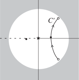
FIG. 1.: The contour for integration is chosen for the correction terms not to dominate the leading terms. In the shaded region, the higher order terms with respect to $\delta$ becomes larger than the leading terms. Hence, the contour is shortened so as not to violate the validity of approximation.

Next we show that $\psi(x)$ given by (52) is actually the solution that satisfies the required boundary condition. In order to evaluate the integration (52) analytically, we use the method of steepest descents. For this method to be valid, $1/|xs_{0}|\ll 1$ is required, where $s_{0}$ is the value of $s$ at the saddle point that dominates the integral. Then, this requirement can be rewritten as

$$|x|>x_{2},$$ (59)

where we must choose $x_{2}$ to satisfy $(1/|xs_{0}|)_{x=x_{2}}\ll 1$. We shall see later that $1/|xs_{0}|$ is of $O(|\tilde{\epsilon}|)$. Hence, for the first time at this moment, we further restrict our consideration to the region in which $\tilde{\epsilon}$ is also small. In order that the condition $|x|>x_{2}$ to be compatible with $|x|<x_{1}$,

$$\left({\kappa\over k_{0}\Omega_{0}}\right)^{2/3}\ll\mbox{min}(1,\kappa^{2}/\kappa_{1}^{2},\kappa\Omega_{1}/\Omega_{0}),$$ (60)

is required. However, this requirement to the model parameters will not reduce the generality of our analysis so much because we are interested in the case that the typical length-scale for the modification of dispersion relation, $k_{0}^{-1}$, is sufficiently small.

As in the case of $\delta$, we introduce an expansion parameter

$$\epsilon:=|\tilde{\epsilon}(x_{2})|,$$ (61)

and we neglect the terms that induce the relative error of $O(\epsilon^{2})$ or smaller in the amplitude of the wave function. As for $\delta$, we also keep the terms up to linear order in $\delta$. Here one remark is in order. We imposed a further restriction $|x|>x_{2}$ to evaluate the explicit form of the solution (52). We stress, however, that the solution (52) itself is valid throughout the region $|x|<x_{1}$.

To evaluate (52) by using the method of steepest descents, we need to know the value of $s$ at saddle points which are determined by solving

$$f^{\prime}(s) \equiv f^{\prime}_{0}(s)+f^{\prime}_{1}(s)$$ (62)

$$= \left[1+{\tilde{\epsilon}^{2}(sx)^{2}\over{2}}-\left(1+{i\omega\over{\kappa}}\right)(sx)^{-1}\right]+(sx)^{-1}W^{(1)}=0.$$ (63)

We solve this equation by assuming that the solution is given by a power series expansion with respect to $\delta$ as

$$s_{\pm}=s_{0\pm}+s_{1\pm}+s_{2\pm}\cdots.$$ (64)

For our present purpose, it is enough to find the solution in the form of series expansion with respect to $\epsilon$. One solution of $xs_{0}$ is of $O(1)$, and the integration along the path through this saddle point cannot be evaluated by the method of steepest descents. The other two solutions are given by

$$xs_{0\pm}:=\mp\left(\sqrt{-\tilde{\epsilon}^{2}\over 2}\right)^{-1}-{1+i\omega/\kappa\over 2}\pm\sqrt{{-\tilde{\epsilon}^{2}\over 2}}{3(1+i\omega/\kappa)^{2}\over 8}+O(\epsilon^{2}),$$ (65)

and

$$xs_{1}= \pm \left(\sqrt{-\epsilon^{2}\over 2}\right)^{-1}\left({\delta_{0}\over 4}-{\delta_{1}\over 4}+\delta_{2}\right)+{1\over 4}\left[\left(3+{i\omega\over\kappa}\right)\delta_{0}+\left(-3+{i\omega\over\kappa}\right)\delta_{1}+8\delta_{2}\right]$$ (66)

$$\mp {1\over 32}\sqrt{-\epsilon^{2}\over 2}\left(1+{i\omega\over\kappa}\right)\left[\left(9+{i\omega\over\kappa}\right)\delta_{0}-3\left(3-{5i\omega\over\kappa}\right)\delta_{1}+4\left(5-{3i\omega\over\kappa}\right)\delta_{2}\right]+O(\epsilon^{2}).$$ (67)

Since $|s_{max}/s_{0\pm}|\sim\sqrt{1/\tilde{\delta}}\gg 1$, these saddle points are contained in the region in which the expansion with respect to $\delta$ is valid. In the following, to keep the notational simplicity, we abbreviate the subscript $\pm$ from $s_{0\pm}$ and $s_{1\pm}$ unless it causes any ambiguity.

Now we evaluate the integration (52) by using the method of steepest descents. For the contour given in Fig. 1, only the saddle point $s_{+}$ dominantly contributes to the integration inside the horizon. For our present purpose, the formula

$$\psi(x)\approx{-\sqrt{2\pi}e^{xf(s_{\pm})}\over{(-xf^{\prime\prime}(s_{\pm}))^{1/2}}}\left[1-{5\over{24}}{(xf^{\prime\prime\prime}(s_{\pm}))^{2}\over{(xf^{\prime\prime}(s_{\pm}))^{3}}}+{1\over 8}{xf^{(4)}(s_{\pm})\over{(xf^{\prime\prime}(s_{\pm}))^{2}}}+O(\epsilon^{2})\right],$$ (68)

is accurate enough to keep the correction up to $O(\epsilon^{1})$. The details of calculation to evaluate Eq. (68) up to $O(\epsilon,\delta)$ is given in Appendix B. In the end, we obtain

$$\psi(x) \approx \sqrt{2\pi\kappa}(k_{0}\Omega_{0})^{-{i\omega\over\kappa}-{1\over 2}}(-2\kappa x)^{-{3\over 4}-{i\omega\over{2\kappa}}}\exp\left(-{2\over 3}\sqrt{2\kappa}k_{0}\Omega_{0}(-x)^{3/2}+W+O(\epsilon^{2},\delta^{2})\right),$$ (69)

where

$$W = -\left(\sqrt{-\tilde{\epsilon}^{2}\over 2}\right)^{-1}\left(-{1\over 10}\tilde{\delta}_{0}+{1\over 10}\tilde{\delta}_{1}-{2\over 5}\tilde{\delta}_{2}\right)$$ (73)

$$+\left({i\omega\over{4\kappa}}+{3\over 8}\right)\tilde{\delta}_{0}+\left({i\omega\over 4\kappa}-{3\over 8}\right)\tilde{\delta}_{1}+{1\over 2}\tilde{\delta}_{2}$$

$$+\sqrt{{-\tilde{\epsilon}^{2}\over 2}}\Biggl{[}\left(-{41\over 48}-{i\omega\over\kappa}-{1\over 4}\left({i\omega\over\kappa}\right)^{2}\right)+\left({11\over 64}+{1\over 4}{i\omega\over\kappa}+{1\over 16}\left({i\omega\over\kappa}\right)^{2}\right)\tilde{\delta}_{0}$$

$$\quad\quad+\left(-{11\over 64}+{3\over 4}{i\omega\over\kappa}+{15\over 16}\left({i\omega\over\kappa}\right)^{2}\right)\tilde{\delta}_{1}+\left(-{5\over 16}-{i\omega\over\kappa}-{3\over 4}\left({i\omega\over\kappa}\right)^{2}\right)\tilde{\delta}_{2}\Biggr{]}.$$

We can immediately see that amplitude of the wave function reduces exponentially as we decrease $x$ (as we increase $-x$).

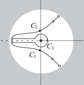
FIG. 2.: The deformed integration contour to evaluate $\psi(x)$ outside the horizon. In $x>0$ region, the saddle points move to the neighborhood of the imaginary axis. The contours $C_{1}$ and $C_{2}$ are chosen to pass through these saddle points and to be able to evaluate the integrations along them by the steepest descents. The remaining part of the integration contour which goes around the branch cut is called $C_{3}$.

Next we turn to evaluate $\psi(x)$ for $x>0$. We use the method of steepest descents again. In the present case, the location of saddle points moves to points on the imaginary axis on the complex $s-$plane. The leading order approximation is given by

$$xs_{0\pm}=\pm{\sqrt{2}i\over\epsilon_{2}}+\cdots.$$ (74)

Therefore, to evaluate (52) by using the method of steepest descents, we need to deform the contour of integration. At this point, we must take account of the existence of a branch cut emanating from $s=0$, which originates from the log-term in the integrand. We choose this branch cut along the negative side of the real axis. Then, deforming the contour so as to go through these two saddle points we find that the contour is divided into three pieces as shown in Fig. 2. We respectively denote them by $C_{1},C_{2}$ and $C_{3}$. $C_{1}$ and $C_{2}$ are the contours passing through the saddle points $s_{-}$ and $s_{+}$, respectively. Both contours have a new boundary point which is chosen to satisfy $|s|<s_{max}$. The contour $C_{3}$ connects these two newly introduced boundary points, going around the origin in the anti-clockwise manner.

First we evaluate the integrations along the contours $C_{1}$ and $C_{2}$ by using the method of steepest descents. Just repeating the same calculation as in the case of $x<0$, these integrations are evaluated as

$$\psi_{1,2}(x)=e^{\mp\pi\omega/2\kappa}{1\over{\sqrt{k_{0}\Omega_{0}}}}(k_{0}\Omega_{0})^{-{i\omega\over\kappa}}\sqrt{2\pi\kappa}(2\kappa x)^{-{3\over 4}-{i\omega\over{2\kappa}}}\exp\left(\mp i{2\over 3}\sqrt{2\kappa}k_{0}\Omega_{0}x^{3/2}+W_{1,2}+O(\epsilon^{2},\delta^{2})\right),$$ (75)

where

$$W_{1,2} = \mp i{\sqrt{2}\over\tilde{\epsilon}}\left(-{1\over 10}\tilde{\delta}_{0}+{1\over 10}\tilde{\delta}_{1}-{2\over 5}\tilde{\delta}_{2}\right)$$ (79)

$$+\left({i\omega\over{4\kappa}}+{3\over 8}\right)\tilde{\delta}_{0}+\left({i\omega\over 4\kappa}-{3\over 8}\right)\tilde{\delta}_{1}+{1\over 2}\tilde{\delta}_{2}$$

$$\mp i{\tilde{\epsilon}\over\sqrt{2}}\Biggl{[}\left(-{41\over 48}-{i\omega\over\kappa}-{1\over 4}\left({i\omega\over\kappa}\right)^{2}\right)+\left({11\over 64}+{1\over 4}{i\omega\over\kappa}+{1\over 16}\left({i\omega\over\kappa}\right)^{2}\right)\tilde{\delta}_{0}$$

$$\quad\quad+\left(-{11\over 64}+{3\over 4}{i\omega\over\kappa}+{15\over 16}\left({i\omega\over\kappa}\right)^{2}\right)\tilde{\delta}_{1}+\left(-{5\over 16}-{i\omega\over\kappa}-{3\over 4}\left({i\omega\over\kappa}\right)^{2}\right)\tilde{\delta}_{2}\Biggr{]}.$$

Next we consider the integral along the $C_{3}$ contour. Here, we divide $xf(s)$ given in Eq. (53) into two parts as

$$x\bar{f}_{0}(s):=xs+\left(-1-{i\omega\over\kappa}\right)\ln s$$ (80)

$$x\bar{f}_{1}(s):={\tilde{\epsilon}^{2}(xs)^{3}\over 6}+xf_{1}(s),$$ (81)

and we expand $e^{x\bar{f}_{1}(s)}$ assuming that $x\bar{f}_{1}(s)$ is small. From the validity of such an expansion, it is required that $|x\bar{f}_{1}(s)|\ll 1$. As for the case with large $|s|$, the integrand becomes exponentially small when $|xs|\gg 1$. There we do not have to mind at all even if $x\bar{f}_{1}(s)$ becomes large negative. In the restricted region satisfying $|xs|\lesssim 1$, it is easy to see that $x\bar{f}_{1}(s)\ll 1$ is always guaranteed. As for the case with small $|s|$, we do not have to consider the situation in which $|s|$ becomes extremely small because there is no requirement on the choice of contour except for being inside the saddle points. For example, if we choose the contour to be $|s|\gtrsim 1$, $|x\bar{f}_{1}(s)|\ll 1$ is guaranteed. Therefore, we find that it is allowed to expand $e^{x\bar{f}_{1}(s)}$ as $1+x\bar{f}_{1}(s)+\cdots$.

After this expansion, introducing a new variable $z$ by $e^{-i\pi}z:=sx$, the integration along $C_{3}$ is written as

$$\psi_{3}(x)\approx x^{i\omega\over\kappa}\int_{\bar{C}_{3}}\,dz\,(-z)^{-1-{i\omega\over\kappa}}e^{-z}[1+x\bar{f}_{1}],$$ (82)

where $\bar{C}_{3}$ is the contour in the complex $z-$plane corresponding to $C_{3}$. Since the integrand becomes exponentially small at the boundaries, we are allowed to continue the contour to $\infty$. Then, using the integral representation of a gamma function, the leading term corresponding to $1$ in the square brackets of Eq. (82) is expressed as

$$\psi_{3}(x)\approx-2\sinh(\pi\omega/\kappa)\Gamma(-i\omega/\kappa)\,x^{i\omega/\kappa}.$$ (83)

Next, we consider the remaining terms in Eq. (82). Let us express $x\bar{f}_{1}$ as $x\bar{f}_{1}=\sum a_{n}(-z)^{n}$, where the coefficients $a_{n}$ are non-dimensional constants. Then, by using the integral representation of the gamma function, we can evaluate the contribution from each term as

$$a_{n}\int_{\bar{C}_{3}}\,dz\,(-z)^{n-1-i\omega/\kappa}e^{-z}=-2a_{n}\sinh\left(\pi\left({\omega\over\kappa}+in\right)\right)\Gamma\left(n-{i\omega\over\kappa}\right),$$ (84)

and we find that its relative order is simply determined by the order of $a_{n}$. Hence, to find the expression correct up to $O(\epsilon^{1},\delta^{1})$, the only term that we must keep is

$$x\bar{f}_{1}(s)\approx-{i\omega\over{2\kappa}}\left({i\omega\over{\kappa}}+1\right)\tilde{\delta}_{1}(sx)^{-1}.$$ (85)

Thus, we finally obtain

$$\psi_{3}(x)=-2\sinh(\pi\omega/\kappa)\Gamma(-i\omega/\kappa)\,x^{i\omega/\kappa}\left(1-{i\omega\over{2\kappa}}\tilde{\delta}_{1}+O(\epsilon^{2},\delta^{2})\right).$$ (86)

In this section, we approximately solved Eq. (37) with the boundary condition that the wave function decreases exponentially inside the horizon. We evaluated the explicit form of the approximate solution in the region $x_{1}>x>x_{2}$ as

$$\psi(x)=\psi_{1}(x)+\psi_{2}(x)+\psi_{3}(x),$$ (87)

where each component $\psi_{i}(x)$ is given by Eq. (75) or Eq. (86). This expression is correct up to $O(\epsilon^{1},\delta^{1})$ .

B the case far from the horizon

In the region far from the horizon, spacetime will become almost flat. In this region we assume that the rate of change of $1/\Omega(x)$ and $v(x)$ is sufficiently small. As we have seen for the asymptotic form of solutions in Sec.2, we have four independent solutions since the ODE (19) is of fourth order. For the solutions with short wavelength corresponding to $k_{\pm}$, we can use WKB approximation to solve Eq. (18). On the other hand, for the solutions with long wavelength corresponding to $k_{\pm s}$, we can solve Eq. (18) perturbatively by treating the correction due to the modification of dispersion relation as small. To be strict, we restrict our consideration to the region $x>x_{2}$, where $x_{2}$ is that given in Eq. (33). In this region, we assume that the following relations

$$\Omega{d\over dx}{1\over\Omega},~{}{1\over v}{d\over dx}v,~{}{1\over(1-v^{2})}{d\over dx}(1-v^{2})\lesssim{\omega\over 1-v^{2}},$$ (88)

are satisfied. As for higher order differentiations, we also assume that they are all restricted like

$$\Omega{d^{2}\over dx^{2}}{1\over\Omega}\lesssim\left({\omega\over 1-v^{2}}\right)^{2},\quad\Omega{d^{3}\over dx^{3}}{1\over\Omega}\lesssim\left({\omega\over 1-v^{2}}\right)^{3},\cdots.$$

By substituting the expansion (35), we find that these conditions are satisfied even in the region close to the horizon.

Here, we define a quantity $\epsilon(x):={\omega\over{k_{0}\Omega(1-v^{2})^{3/2}}}$, which reduces to $\tilde{\epsilon}(x)$ near the horizon. It will be natural to assume that $\epsilon(x)$ takes its largest value in the region close to the horizon, and hence $\epsilon(x)$ is at most of $O(\epsilon^{1})$ owing to the restriction $x>x_{2}$. In the following, we construct approximate solutions valid up to $O(\epsilon^{1})$ in the sense of $\delta\psi/\psi$.

We begin with considering the solutions with short wavelength. Substituting the expression

$$\psi=e^{i\int^{x}dx^{\prime}\,k(x^{\prime})},$$ (89)

into Eq. (19), we write down the equation for $k(x)$. Neglecting the terms on which differentiations with respect to $x$ acted more than three times,

$${\left(1\over{{k_{0}}{\Omega}}\right)}^{2}k^{4}-(1-v^{2})k^{2}-2v{\omega}k+{\omega}^{2} \approx i{d\over{dx}}\left[2{\left(1\over{{k_{0}}{\Omega}}\right)}^{2}k^{3}-(1-v^{2})k-v{\omega}\right]$$ (92)

$$+{3k^{\prime}{}^{2}+4kk^{\prime\prime}\over k_{0}^{2}\Omega^{2}}+{12kk^{\prime}\over k_{0}^{2}\Omega}\left({d\over dx}{1\over\Omega}\right)$$

$$+{5k^{2}\over 2k_{0}^{2}}\left(\left({d\over dx}{1\over\Omega}\right)^{2}+{1\over\Omega}\left({d^{2}\over dx^{2}}{1\over\Omega}\right)\right),$$

is obtained, where $~{}^{\prime}~{}$ is used to represent a differentiation with respect to $x$. Denoting the left hand side of Eq. (92) by $F(k)$, we find that the first term on the right hand side is expressed as

$${i\over 2}{d\over dx}\left({dF(k)\over dk}\right).$$

We denote the remaining terms on the right hand side by $G(k)$. Following the standard prescription of the WKB approximation, the terms which contain differentiations with respect to $x$ is taken to be small. Accordingly, we also expand $k(x)$ in accordance with the number of differentiation as

$$k(x)=k^{(0)}(x)+k^{(1)}(x)+k^{(2)}(x)+\cdots.$$ (93)

After a slightly long but a straight forward calculation, we obtain

$$k_{\pm}^{(0)} = \pm k_{0}\Omega\sqrt{1-v^{2}}\left(1\pm v\epsilon(x)-{1+2v^{2}\over 2}\epsilon^{2}(x)+O(\epsilon^{3})\right)$$ (94)

$$= \pm k_{0}\Omega\sqrt{1-v^{2}}+{v\omega\over 1-v^{2}}\mp{(1+2v^{2})\omega^{2}\over{2k_{0}\Omega(1-v^{2})^{5/2}}}+\cdots,$$ (95)

$$k_{\pm}^{(1)} = {i\over 2}{d\over{dx}}{\ln}\left(\pm k_{0}\Omega(1-v^{2})^{3/2}(1\pm 4v\epsilon(x)+O(\epsilon^{2}))\right)$$ (96)

$$= {i\over 2}{d\over{dx}}{\ln}\left(\pm k_{0}\Omega(1-v^{2})^{3/2}+4vw+\cdots\right),$$ (97)

$$k_{\pm}^{(2)} = \pm k_{0}\Omega\sqrt{1-v^{2}}\Biggl{\{}{\epsilon^{2}(x)\over 8\omega^{2}}\Biggl{[}41v^{2}v^{\prime}{}^{2}+(1-v^{2})\left(14(vv^{\prime})^{\prime}+18vv^{\prime}\Omega\left({1\over\Omega}\right)^{\prime}\right)$$ (99)

$$\hskip 85.35826pt+(1-v^{2})^{2}\left(4\Omega\left({1\over\Omega}\right)^{\prime\prime}+\biggr{[}\Omega\left({1\over\Omega}\right)^{\prime}\biggr{]}^{2}\right)\Biggr{]}+O(\epsilon^{3})\Biggr{\}}.$$

Now we turn to the solutions with small absolute values, i.e., $k_{\pm s}$. In this case, we cannot use the WKB approximation because the wavelength is not necessarily short compared with the typical scale for the background quantities to change. However, for the model with the standard dispersion relation, we have exact solutions for the field equation $k_{\pm s}=\pm\omega/(1\pm v)$. We can use them as the leading order approximation, which is solutions when we neglect the terms related to the modification of dispersion relation. If we substitute $k_{\pm s}\approx\pm\omega/(1\pm v)$ into the neglected terms, we find that all of them have relative order higher than $\epsilon^{2}$. At first glance, one may think that the terms corresponding to the second and third terms in the square brackets in Eq. (92) give a correction of $O(\epsilon^{0})$, but they mutually cancel out. As a result, the equation to determine the correction $\delta k_{\pm s}:=k_{\pm s}\mp\omega/(1\pm v)$ is obtained as

$$-i\partial_{x}(1-v^{2})\delta k_{\pm s}\pm 2\omega\delta k_{\pm s}={1\over 2k_{0}^{2}}e^{-i\int^{x}k_{\pm s}^{(0)}(x^{\prime})dx^{\prime}}\left[\partial_{x}^{2}{1\over\Omega}\partial_{x}{1\over\Omega}\partial_{x}+\partial_{x}{1\over\Omega}\partial_{x}{1\over\Omega}\partial_{x}^{2}\right]e^{i\int^{x}k_{\pm s}^{(0)}(x^{\prime})dx^{\prime}}=:H_{\pm}(x).$$ (100)

The right hand side consists of the terms related to the modification of dispersion relation, and they are small of $\omega k_{+s}^{(0)}\times O(\epsilon^{2})$. Different from the case for short wavelength modes, the equation to determine the correction becomes a differential equation. Therefore, we can say that the correction stays of $O(\epsilon^{2})$ only when we are interested in the behavior of the solution within a small region such as $x_{1}>x>x_{2}$. Once an extended region is concerned, there is no reason why the correction stays of $O(\epsilon^{2})$. In fact, we need to know the behavior of the solution both at infinity and in the matching region $x_{1}>x>x_{2}$. In such a case, the correction much larger than $O(\epsilon^{2})$ can appear as explained in detail in Appendix C.

Nevertheless, the origin of this correction is the effect of scattering due to the modified dispersion relation. Even if the observed spectrum of the emitted particles deviates from the thermal one due to this effect, it is still possible to adopt the interpretation that the spectrum is modified by the scattering during the propagation to a distant observer though it was initially thermal. Hence, we think that this effect should be discussed separately from the present issue.

However, to be precise, we consider the case that the condition (88) replacing $\lesssim$ with $\ll$ is satisfied. This is the case when $\omega$ is sufficiently large or when the functions $v(x)$ and $1/\Omega(x)$ rapidly converge to some constants at $x\gtrsim x_{1}$. In such cases, we can think of the first term on the left hand side of Eq. (100) as small. Then, solving Eq. (100) iteratively, we find that the correction stays of $O(\epsilon^{2})$. Therefore, we obtain

$$k_{\pm s}\approx\pm{\omega\over 1\pm v}(1+O(\epsilon^{2})).$$ (101)

Consequently, we find that the solutions which behave like $e^{ik(x\to\infty)x}$ at infinity are given by

$${\psi}_{\pm}(x)=e^{i\int^{x}k_{\pm}(y)dy},\quad\quad\psi_{\pm s}(x)=e^{i\int^{x}k_{\pm s}(y)dy},$$ (102)

where the integral constants are chosen appropriately. Here we recall that what we wish to know is not $k(x)$ but $\int^{x}dy\,k(y)$. Although we are keeping track of the error in the expression of $k(x)$, we cannot evaluate the error in the integral $\int^{x}_{\infty}k(y)dy$ when it is integrated from $\infty$ to the matching region where $x_{1}>x>x_{2}$. To overcome this difficulty, we need to make use of the existence of a conserved current

$$j=A(k(x))e^{-2\int^{x}k_{(I)}(y)dy},$$ (103)

where

$$A(k(x))= \omega v+(1-v^{2})k_{(R)}$$ (106)

$$-{1\over k_{0}^{2}\Omega^{2}}\left\{2k_{(R)}(k_{(R)}^{2}-k_{(I)}^{2})+4k_{(R)}\partial_{x}k_{(I)}+2k_{(I)}\partial_{x}k_{(R)}-\partial_{x}^{2}k_{(R)}\right\}$$

$$+{2\over k_{0}^{2}}\left({1\over\Omega}\left({1\over\Omega}\right)^{\prime}\right)\left(-2k_{(R)}k_{(I)}+\partial_{x}k_{(R)}\right)+{1\over 2k_{0}^{2}}\left({1\over\Omega}\left({1\over\Omega}\right)^{\prime}\right)^{\prime}k_{(R)},$$

and $k_{(R)}$ and $k_{(I)}$ are the real and the imaginary parts of $k$, respectively. The derivation of $j$ is given in Appendix D.

We evaluate this conserved current $j$ at $x\to\infty$, where all terms that contain differentiations with respect to $x$ vanish there. Adopting the normalization $|\phi|^{2}=1$ at $x\to\infty$, $j$ is determined as

$$j=\omega v_{\infty}+(1-v_{\infty}^{2})k_{\infty}-{2\over k_{0}^{2}\Omega_{\infty}^{2}}k_{\infty}^{3}.$$ (107)

For $l=\pm,\pm s$, by substituting $k_{l\infty}$ into the expression of $j$ in place of $k_{\infty}$, we also define the conserved current $j_{l}$ corresponding to $k_{l}$.

Owing to the conservation of $j$,

$$\psi_{l}(x)=\sqrt{j_{l}\over A(k_{l}(x))}e^{i\int^{x}k_{l(R)}(y)dy}.$$ (108)

By using this improved expression, we can calculate the explicit form of $\psi_{l}(x)$ in the region $x_{1}>x>x_{2}$ without any ambiguity except for the constant phase factor that does not alter the absolute magnitude of the wave function. Expanding the expression (108) in powers of $\tilde{\delta}_{i}$ with the substitution of Eqs. (35), we evaluate $\psi_{l}(x)$ keeping the terms up to $O(\delta^{1})$. Here in evaluating $A(x)$, the terms that include $k_{(I)}$ becomes higher order in $\epsilon$, and hence we can neglect them all. Consequently, we obtain

$${\psi_{\pm}(x)\over\sqrt{j_{\pm}}}={e^{i\alpha_{\pm}}\over{\sqrt{k_{0}\Omega_{0}}}}(2\kappa x)^{-{3\over 4}-{i\omega\over{2\kappa}}}\exp\left(\pm i{2\over 3}k_{0}\Omega_{0}\sqrt{2\kappa}x^{3\over 2}+W_{\pm}+O(\epsilon^{2},\delta^{2})\right),$$ (109)

$${\psi_{+s}(x)\over\sqrt{j_{+s}}}=e^{i\alpha_{+s}}x^{i\omega\over\kappa}\exp\left(-{i\omega\over{2\kappa}}\tilde{\delta}_{1}+O(\epsilon^{2},\delta^{2})\right),$$ (110)

where $W_{+}$ and $W_{-}$ are no different from $W_{2}$ and $W_{1}$ in Eq. (79), respectively. As noted above, there appears an integration constant $\alpha_{l}$ that cannot be determined by the present analysis, but it is guaranteed to be a real number. Here, we did not give the explicit form of $\psi_{-s}$ because we do not use it later.

By comparing (87) with (110), we find that the solution (87) obtained in the region close to the horizon is matched to the solutions obtained in the outer region like

$$\psi(x)=\sqrt{2\pi\kappa}\left(e^{-{\pi\omega\over{2\kappa}}+i\alpha^{\prime}_{-}}{\psi_{-}\over\sqrt{j_{-}}}+e^{{\pi\omega\over 2\kappa}+i\alpha^{\prime}_{+}}{\psi_{+}\over\sqrt{j_{+}}}\right)-2\sinh\left({\pi\omega\over\kappa}\right)\Gamma\left(-{i\omega\over\kappa}\right)e^{i\alpha_{+s}}{\psi_{+s}\over\sqrt{j_{+s}}},$$ (111)

where $\alpha^{\prime}_{\pm}$ are also real constants. From this expression, we can read the coefficients $c_{+s},c_{-}$ as

$$c_{+s}=-2\sinh\left({\pi\omega\over\kappa}\right)\Gamma\left(-{i\omega\over\kappa}\right){e^{i\alpha_{+s}}\over\sqrt{j_{+s}}}(1+O(\epsilon^{2},\delta^{2}))$$ (112)

$$c_{-}=\sqrt{2\pi\kappa}e^{-{\pi\omega\over{2\kappa}}}{e^{i\alpha^{\prime}_{-}}\over\sqrt{j_{-}}}\left(1-{4v\omega\over{k_{0}\Omega}}(1-v^{2})^{-3/2}\right)^{-1/2}(1+O(\epsilon^{2},\delta^{2})).$$ (113)

The factor $\omega^{\prime}v_{g}$ appears in the formula (30) for the expectation value of the created particles. By differentiating the dispersion relation at infinity (22) with respect to $k_{\infty}$, this factor is easily calculated as

$$\omega^{\prime}(k_{\infty})v_{g}(k_{\infty}):=(\omega-vk_{\infty}){d\omega(k_{\infty})\over dk_{\infty}}=v_{\infty}\omega+(1-v_{\infty}^{2})k_{\infty}-{2k_{\infty}^{3}\over k_{0}^{2}\Omega_{\infty}^{2}},$$ (114)

and we find it to coincide with the conserved current. Thus, by considering the combination of $\omega^{\prime}(k_{+s})v_{g}(k_{+s})|c_{+s}|^{2}$ the factor $j_{+s}$ in $c_{+s}$ cancels, and the same is also true for $k_{-}$. Finally the expectation value of the number of created particle is evaluated as

$$N(\omega)={1\over{e^{2\pi\omega/\kappa}-1}}(1+O(\epsilon^{2},\delta^{2})).$$ (115)

V analytic and numerical studies of the deviation from hawking spectrum

	$~{}~{}\epsilon^{-1}~{}~{}$	$~{}~{}\epsilon^{0}~{}~{}$	$~{}~{}\epsilon^{1}~{}~{}$	$~{}~{}\epsilon^{2}~{}~{}$
$\delta^{0}$	$x^{3/2}$	$x^{0}$	$x^{-3/2}$	$x^{-3}$
$\delta^{1}$	$x^{5/2}$	$x^{1}$	$x^{-1/2}$	$x^{-2}$
$\delta^{2}$	$x^{7/2}$	$x^{2}$	$x^{1/2}$	$x^{-1}$
$\delta^{3}$	$x^{9/2}$	$x^{3}$	$x^{3/2}$	$x^{0}$

TABLE I. Table to explain the matching procedure.

In the preceding section, to obtain the flux of the created particles observed in the asymptotic region, where $v(x)$ is essentially constant, we propagated the near-horizon solution (87), which satisfies the appropriate boundary condition, to the infinity by matching it with the outer-region solutions (110), which are valid in the region distant from the horizon. As a result, we could determine the coefficients $c_{l}$ and we found that the thermal spectrum is reproduced up to $O(\epsilon^{1},\delta^{1})$.

To explain the matching procedure in more detail, here we present a table. In the construction of the near-horizon solution, the equation to be solved was expanded with respect to $\delta$, and we obtained an equation which correctly determines the terms up to $O(\delta^{1})$. These terms correspond to the first two lines in the above table. Then, expanding them with respect to $\epsilon$ by restricting our consideration to the region $x_{2}<x<x_{1}$, we obtained the expression (87) with (75) and (86), which contains the terms corresponding to the first $2\times 3$ elements in the table.

On the other hand, in the region distant from the horizon, we first considered an expansion of the solution with respect to $\epsilon$, and calculated the corrections up to $O(\epsilon^{1})$. Namely, the terms corresponding to the first three columns in the above table are obtained. As the next step, in the region of $x_{2}<x<x_{1}$, we expanded this expression also with respect to $\delta$ up to $O(\delta^{1})$ by substituting (35) into Eq. (79), and we obtained the first $2\times 3$ elements in the table. The expressions that we finally obtained are the outer-region solutions (110).

Such two fold expansions in both schemes are simultaneously valid only in the region $x_{1}<x<x_{2}$, where both $\tilde{\epsilon}(x)$ and $\tilde{\delta}_{i}(x)$ are small. As mentioned above, as long as $k_{0}$ is taken to be sufficiently large, this overlapping region always exists. Since both expressions obtained by using the above two different schemes are approximate solutions of the same equation, they must be identical if we take an appropriate superposition of the four independent solutions. In fact, we found that the near-horizon solution (87) can be written as a superposition of the outer-region solutions as given in Eq. (111). Now, let us look at the above table again. For each element in the table, we have assigned a power of $x$ that the corresponding terms possess. As we mentioned above, we need to choose an appropriate superposition of the four independent outer-region solutions to achieve a successful matching. The coefficients which determine the weight of this superposition is nothing but $c_{l}$. Now we should note that the condition to determine the coefficients $c_{l}$ will be completely supplied by matching the $x$-independent elements. Once these coefficients are determined, the agreement of the other $x$-dependent terms must be automatic from the consistency. The leading order $x$-independent elements consists of the terms of $O(\epsilon^{0}\delta^{0})$, and it is easy to see that the second lowest one consists of the terms of $O(\epsilon^{2}\delta^{3})$. This fact tells us that the possible modification of the coefficients $c_{+s}$ and $c_{-}$ is at most of $O(\epsilon^{2}\delta^{3})$, and hence the possible deviation from the thermal radiation starts only from this order. Thus we find

$$N(\omega)={1\over{e^{2\pi\omega/\kappa}-1}}(1+O(\epsilon^{2}\delta^{3})).$$ (116)

Next we investigate the deviation from thermal radiation $\delta N/N:=(N-N_{thermal})/N_{thermal}$ in more detail. There are three different quantities of $O(\delta)$ as given in (31). We write them down as

$$\tilde{\delta}_{0}=xv^{\prime}|_{x=0}=\kappa x,\quad\tilde{\delta}_{1}=x\kappa^{-1}v^{\prime\prime}|_{x=0}=:(\kappa x)b_{1},\quad\tilde{\delta}_{2}=x\Omega_{0}\left({1\over\Omega}\right)^{\prime}_{x=0}=:(\kappa x)b_{2},$$ (117)

where we introduced non-dimensional model parameters $b_{1}$ and $b_{2}$. We also have various quantities of $O(\delta^{2})$ and of $O(\delta^{3})$ consisted of higher derivatives of $v$ and $1/\Omega$. They are

$$x^{2}\kappa^{-1}v^{\prime\prime\prime}|_{x=0}=:(\kappa x)^{2}b_{3},\quad\quad x^{2}\Omega_{0}\left({1\over\Omega}\right)^{\prime}_{x=0}=:(\kappa x)^{2}b_{4},$$ (118)

and

$$x^{3}\kappa^{-1}v^{(4)}|_{x=0}=:(\kappa x)^{3}b_{5},\quad\quad x^{3}\Omega_{0}\left({1\over\Omega}\right)^{\prime\prime}_{x=0}=:(\kappa x)^{3}b_{6},$$ (119)

respectively. Also, $b_{3}$, $b_{4}$, $b_{5}$ and $b_{6}$ are non-dimensional model parameters. One may suspect that terms including factors proportional to $\kappa^{-2}$ such as $x\kappa^{-2}v^{\prime\prime\prime}|_{x=0}$ might appear among the correction terms of $O(\epsilon^{2}\delta^{3})$. However, by repeating the same calculation that was given in Sec.4 with extra higher order derivative terms, we can verify that such factors do not appear. From this notion, we can expect that the deviation from the thermal spectrum is given by

$${\delta N\over N}={\kappa^{2}\over k_{0}^{2}\Omega_{0}^{2}}\Biggl{[} \left(a_{000}+a_{001}b_{1}+a_{002}b_{2}+(\mbox{7 other terms})\right)$$ (121)

$$+\left(a_{03}+a_{13}b_{1}+a_{23}b_{2}\right)b_{3}+\left(a_{04}+a_{14}b_{1}+a_{24}b_{2}\right)b_{4}+a_{5}b_{5}+a_{6}b_{6}\Biggr{]}+O(\epsilon^{4}\delta^{6}),$$

where “$a$”s are some functions of $\omega/\kappa$ which are independent of model parameters.

Now, we numerically confirm that the deviation actually starts from this order. The following results are obtained by using MATHEMATICA. As an example, let us consider a model given by

$$v = -{1\over 2}e^{-2x-3x^{2}}-{1\over 2},$$ (122)

$$\Omega = 9e^{-x-x^{2}/2}+1.$$ (123)

For this model, we have $\kappa=1$, $b_{1}=1$ and $b_{2}=9/10$, and the other parameters also do not vanish. For this fixed model, we numerically calculated the deviation from the thermal spectrum for various values of $1/k_{0}^{2}$. The frequency $\omega$ was fixed to 1 since our main interest is in the modes whose observed frequency at infinity becomes comparable with Hawking temperature ($=\kappa/2\pi$). The results of the numerical calculation are shown in Fig.3 by the filed circles. The horizontal axis is $\log(1/k_{0})$ and the vertical one is $\log\delta N/N$. The data points are fitted well by a liner function (the solid line) with its gradient, $1.99742$, which perfectly agrees with the expectation represented by Eq.(121).

At this point, one may notice that the deviation we obtained here is much larger than that given by Corley and Jacobson[5], in which a model with

$$v={1\over 2}\{\tanh[(2\kappa x)^{2}]\}^{1/2}-1,$$ (124)

and $\Omega\equiv 1$ was considered . The outstanding feature of their model is that $b_{1}=b_{2}=b_{3}=b_{4}=b_{5}=b_{6}=0$. Hence, the terms of $O(\epsilon^{2}\delta^{3})$ in Eq.(121) reduce to $a_{000}{\kappa^{2}/k_{0}^{2}\Omega_{0}^{2}}$. If $a_{000}\equiv 0$, all the terms of $O(\epsilon^{2}\delta^{3})$ in the deviation $\delta N/N$ disappear, and it turns out to be $O(\epsilon^{4}\delta^{6})$. If so, the discrepancy between two calculations can be understood. To show that this is certainly the case, we repeated the numerical calculation for the same model that was discussed in Ref.[5]. The resulting $\delta N/N$ calculated for various values of $1/k_{0}$ were also plotted in Fig.3 by the open squares. Again, the data points in logarithmic plot are fitted well by a linear function. But, this time, its gradient is 4.06935, which indicates that the deviation is actually caused by the terms of $O(\epsilon^{4}\delta^{6})$.

Now, we can conclude that $a_{000}\equiv 0$. Although this result might be interesting, we do not pursue this direction of study in this paper. Here, we would like to focus on another interesting aspect that is anticipated by the expression (121). With moderate values of model parameters, the deviation $\delta N/N$ stays small for a sufficiently large $k_{0}$. However, conversely, we can expect that the deviation from the thermal spectrum becomes large if we consider some extreme modifications of the special reference frame. Especially, when we consider the limiting case in which $\Omega_{0}^{2}\to 0$, the expression (121) diverges. Although the approximation used to obtain the analytic expression (121) is no longer valid in this limit, we can still expect that the resulting spectrum will significantly differ from the thermal one. As we mentioned below Eq.(10), there is a lower bound on $\Omega^{2}(x)$. The possible smallest value of $\Omega^{2}(x)$ is $1-\tilde{v}^{2}$, which is realized when $v(x)=0$. Hence, we find $v(x)\approx 0$ near $x=0$ in this limiting case. Recall that $v(x)$ was the coordinate velocity of the integration curves of $u$. Hence, vanishing $v(x)$ means that we adopt the reference frame corresponding to the static observers.

Here, we present the results of our numerical calculation, which shows that the deviation $\delta N/N$ can be large for some cases. Since we also want to demonstrate that the drastic change of spectrum can occur just in the consequence of the change of the special reference frame, we varies only the function $\gamma(\tilde{x})$, which was defined in Eq.(4). The model of $\tilde{v}(\tilde{x})$ is kept unchanged. As for a model of $\tilde{v}(\tilde{x})$, we assume the same form that is given in Eq.(122). As for $\gamma(\tilde{x})$, we adopt

$$\gamma={-\tilde{v}-(1/2)\over\rho^{-1}-\tilde{v}},$$ (125)

with $\rho\in[0,1)$. $\rho=0$ corresponds to the original model associated with the freely falling observers, and $\rho=1$ corresponds to the case with $\Omega_{0}^{2}=0$. With this choice of $\gamma(\tilde{x})$, the following two conditions are satisfied. One is that $v(x)$ stays negative for all positive $x$. The other is that $\Omega_{\infty}^{2}=1$. We calculated the deviation $\delta N/N$ for various values of $\rho$, and the results were shown in Fig.4. As was expected, the deviation becomes large for small $\Omega_{0}^{2}$. This plot raises an interesting speculation that $N$ might converge to $0$ in the $\Omega_{0}^{2}\to 0$ limit. Although we have not confirmed it yet, it is very likely that this is the case because the situation in this limit is very similar to the case in which we set a static mirror surrounding the event horizon of the black hole. The calculation for small $\Omega_{0}^{2}$ were tried, but it was found to be out of validity of our present computation code. Anyway, we conclude that, even if $\kappa/k_{0}$ is sufficiently small, the deviation from the thermal spectrum can be large if the combination $\kappa/k_{0}\Omega_{0}$ becomes large. It should be noted that the integration curves of $u$ are not required to be suffered from infinite acceleration to achieve such a small but non-zero $\Omega_{0}^{2}$.

FIG. 3.: The logarithmic plot of $\delta N/N$ as a function of $1/k_{0}$ for two different choice of $v(x)$. The filled circles(our model) and the open squares(model in Ref.[5]) represent the numerical data points for respective models. Each solid line corresponds to a linear function which fits the data points.

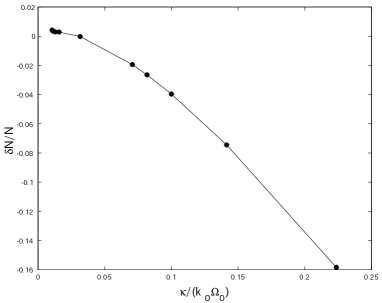
FIG. 4.: A plot of $\delta N/N$ as a function of $1/\Omega_{0}$ for the model given by Eq.(5.6).

VI Conclusion

We studied the particle creation in a model which is a generalization of the Unruh’s toy model. In his model, the field equation for a scalar field is modified by introducing a non-standard dispersion relation. To do so, we necessarily violates the Lorentz invariance. This radical change of theory is originally motivated by the possible existence of the effect due to the unknown physics at Planck scale. However, as is explained in Introduction, there is another point of view, on which it is also meaningful to study this model as an effective theory which takes into account the interaction between various fields even if we believe that the Lorentz invariance is exact,

In the original model, the dispersion relation is modified on the basis of the freely falling observers. In our present work, we generalized the choice of the reference frame with respect to which we set the non-standard dispersion relation. Extending the analytic method developed by Corley [6], we have shown that the thermal spectrum of radiation from a black hole is almost reproduced as long as the modification of the special reference frame is not too extreme. In this analysis, we assumed $\omega\approx\kappa$, where $\omega$ is the frequency of the emitted photon observed at the spatial infinity and $\kappa$ is the surface gravity of the black hole. We have also obtained a strong suggesting that the deviation from the exact thermal spectrum appears from $O(\kappa^{2}/k_{0}^{2})$, where $k_{0}$ is the typical wave number corresponding to the modification of the dispersion relation. This speculation has been confirmed numerically.

Of course, we should not stress this small deviation from the Hawking spectrum. In the ordinary model with the Lorentz invariant dispersion relation, the thermal radiation at the temperature $T$ for the static observer is observed as the thermal radiation at the temperature $\sqrt{1-\beta\over 1+\beta}T$ for the observer moving with the radial velocity $\beta$. This argument holds in general whatever the source of the outward pointing radiation is because it is a direct consequence of $\omega=k$. However, in the present modified model, the Lorentz invariance is violated from the beginning. We can easily see that $(\omega-k)/\omega$ is also of $O(\omega^{2}/k_{0}^{2})$. Hence, even if the exact Hawking spectrum is reproduced for one specific free-falling observer, it cannot be so for the other free-falling observers.

On the other hand, the result that we obtained analytically also suggests that the deviation from the thermal spectrum can be large if we consider some extreme situations. With the aid of numerical methods, we also examined one of such extreme situations. We considered a sequence of different special reference frames which ranges from the case in which the observers associated with the special reference frame are freely falling into black hole to the case in which they are kept from falling into it. We found that, in the latter limiting case, the spectrum of radiation can significantly differ from the thermal one, even though $\omega^{2}/k_{0}^{2}$ is small. It will be important to study the physical meaning of this result. But, since the central issue of this paper is to develop the analytic treatment of our new model, we have not performed detailed numerical studies yet. We will return to this issue in future publications.

A the contour modified for the correction term

In this appendix, we explain how we choose the contour of integration $C$ in Eq. (52) in more detail. As shown in Ref. [6], the contour $C$ in Fig. 5 satisfies the condition that the wave function exponentially decreases inside the horizon when $W^{(1)}$ and higher order corrections are neglected. When $W^{(1)}$ are taken into account, however, the contour of integration needs to be modified. The correction $W^{(1)}$, contains the terms proportional to $s^{5}$, while the terms of the highest power in the main component $W^{(0)}$ is proportional to $s^{3}$. As a result, $|W^{(1)}|$ becomes larger than $|W^{(0)}|$ when $|s|$ becomes large. Hence, from the validity of approximation, the contour of integration must be modified to be contained in the region that satisfies the condition $|W^{(0)}|\gg|W^{(1)}|$. By comparing the absolute value of the $s^{3}$ term in $W^{(0)}$ with that of the $s^{5}$ terms in $W^{(1)}$, the allowed region for the contour to move is found to be restricted by

$$|s|<s_{max}=\mbox{min}\left(k_{0}\Omega_{0},k_{0}\Omega_{0}\sqrt{\kappa^{2}\over{\kappa_{1}^{2}}},k_{0}\Omega_{0}\sqrt{\kappa\Omega_{1}\over\Omega_{0}}\right),$$ (A1)

Thus, we modify the contour not to run into infinity but to terminate at points contained in the region $|s|<s_{max}$ as shown in Fig. 1.

Because of this modification of the contour of integration, the boundary terms in Eq. (39) no longer vanish. However, since $\hat{\psi}(s_{max})$ is exponentially small at both end points, we can expect that the correction due to the boundary terms is negligiblly small.

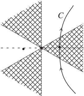
FIG. 5.: The integration contour satisfying the boundary condition that the wave function decays exponentially fast inside the event horizon when the terms of higher order in $\delta$ can be neglected. In the directions indicated by hatched regions, $\hat{\psi}(s)$ increases exponentially. Filled circles represent the saddle points $s_{\pm}$ and the dashed line represents the branch cut.

B evaluation of integration about saddle points

In this appendix, we explain the details how to evaluate Eq. (68). We first consider the exponent $xf(s_{+})$. We evaluate it as an expansion around $s=s_{0}$ like

$$xf(s_{+})= xf_{0}(s_{0})+f^{\prime}_{0}(s_{0})(xs_{1})+{1\over 2x}f^{\prime\prime}_{0}(s_{0})(xs_{1})^{2}+\cdots$$ (B2)

$$+xf_{1}(s_{0})+f^{\prime}_{1}(s_{0})(xs_{1})+{1\over 2x}f^{\prime\prime}_{1}(s_{0})(xs_{1})^{2}+\cdots.$$

The first term in the first line of the right hand side is zeroth order in $\delta$, and the second term vanishes identically. The other terms in the first line are quadratic or higher order in $\delta$. The terms in the second line are proportional to $\delta^{1},\delta^{2},\delta^{3},\cdots$, respectively. Thus we find

$$xf(s_{+})=xf_{0}(s_{0})+xf_{1}(s_{0})+O(\delta^{2}).$$ (B3)

Using Eqs. (55), (58) and (65), $xf(s_{+})$ is found to be given by

$$xf(s_{+}) = -\left(\sqrt{{-\tilde{\epsilon}^{2}\over 2}}\right)^{-1}\left({2\over 3}-{1\over{10}}\tilde{\delta}_{0}+{1\over{10}}\tilde{\delta}_{1}-{2\over 5}\tilde{\delta}_{2}\right)$$ (B7)

$$+{\tilde{\delta}_{0}\over 4}\left(3+i{\omega\over{\kappa}}\right)-{\tilde{\delta}_{1}\over 4}\left(3-i{\omega\over{\kappa}}\right)+2\tilde{\delta}_{2}-\left(1+i{\omega\over{\kappa}}\right)\log(k_{0}\Omega_{0}\sqrt{-2\kappa x})$$

$$+{1\over 4}\left(1+i{\omega\over{\kappa}}\right)\sqrt{{-\tilde{\epsilon}^{2}\over 2}}\left[-\left(1+i{\omega\over{\kappa}}\right)+{\tilde{\delta}_{0}\over 4}\left(9+i{\omega\over{\kappa}}\right)-{\tilde{\delta}_{1}\over 4}\left(9-15i{\omega\over{\kappa}}\right)+\tilde{\delta}_{2}\left(5-3i{\omega\over{\kappa}}\right)\right]$$

$$+O(\delta^{2},\epsilon^{2}).$$

Next, we evaluate $f^{\prime\prime}(s_{+})$. Again we expand it around $s=s_{0}$ as

$${1\over x}f^{{}^{\prime\prime}}(s_{+})= {1\over x}f^{\prime\prime}_{0}(s_{0})+{1\over x^{2}}f^{\prime\prime\prime}_{0}(s_{0})(xs_{1})+\cdots$$ (B9)

$$+{1\over x}f^{\prime\prime}_{1}(s_{0})+{1\over x^{2}}f^{\prime\prime\prime}_{1}(s_{0})(xs_{1})+\cdots.$$

The power indices with respect to $\delta$ of the respective terms in the first line on the right hand side are $0,1,\cdots$. Those in the second line are $1,2,\cdots$. Hence, the expression for $f^{{}^{\prime\prime}}(s_{+})/x$ which is correct up to $O(\delta)$ is given by

$${1\over x}f^{\prime\prime}(s_{+})\approx{1\over x}f^{\prime\prime}_{0}(s_{0})+{1\over x^{2}}f^{\prime\prime\prime}_{0}(s_{0})(xs_{1})+{1\over x}f^{\prime\prime}_{1}(s_{0}).$$ (B10)

As for this factor, it is not necessary to find the second order correction in $\epsilon$. Hence, we can use the truncated expressions for $xs_{0}$ and $xs_{1}$ obtained by discarding the terms of $O(\epsilon)$ in Eqs. (65) and (67). Substituting these into (B10), we find

$${1\over x}f^{\prime\prime}(s_{+})=2\sqrt{{-\tilde{\epsilon}^{2}\over{2}}}\left[1+{3\over 4}\tilde{\delta}_{0}-{3\over 4}\tilde{\delta}_{1}+3\tilde{\delta}_{2}+\sqrt{{-\tilde{\epsilon}^{2}\over{2}}}\left(1+i{\omega\over{\kappa}}\right)\left(1+{3\over 2}\tilde{\delta}_{0}-{3\over 2}\tilde{\delta}_{1}+6\tilde{\delta}_{2}\right)+O(\epsilon^{2},\delta^{2})\right].$$ (B11)

Finally, we evaluate the second and third terms in the square brackets on the right hand side of Eq. (68). As before, we write $f^{\prime\prime\prime}(s_{+})/x^{2}$ as

$${1\over x^{2}}f^{\prime\prime\prime}(s_{+}) = {1\over x^{2}}f^{\prime\prime\prime}_{0}(s_{0})+{1\over x^{3}}f^{(4)}_{0}(s_{0})(xs_{1})+\cdots$$ (B13)

$${1\over x^{2}}f^{\prime\prime\prime}_{1}(s_{0})+{1\over x^{3}}f^{(4)}_{1}(s_{0})(xs_{1})+\cdots.$$

We evaluate the order of each term on the right hand side in this equation. Then, we find that the respective terms in the first line are of $O(\epsilon^{2}),O(\epsilon^{3}\delta),O(\epsilon^{3}\delta^{2}),O(\epsilon^{3}\delta^{3}),\cdots$. Those in the second line are of $O(\epsilon^{2}\delta),O(\epsilon^{2}\delta^{2}),O(\epsilon^{2}\delta^{3}),\cdots$. One may notice that the order in the first line does not change regularly. This is because the second term in the last line in Eq. (55) vanishes if it is differentiated more than four time. Since the leading term in $f^{{}^{\prime\prime}}(s_{+})/x$ is $O(\epsilon^{1})$, we can neglect the terms of $O(\epsilon^{3})$ or higher in Eq. (B13). Furthermore, we do not have to keep the terms of $O(\delta^{2})$ or higher. Therefore, we have only to retain the terms $f^{\prime\prime\prime}_{0}(s_{0})/x^{2}$ and $f^{\prime\prime\prime}_{1}(s_{0})/x^{2}$. Substituting $xs_{0+}\approx-(-\tilde{\epsilon}^{2}/2)^{-1/2}$ into these two terms, $(xf^{\prime\prime\prime}(s_{+}))^{2}/(xf^{\prime\prime}(s_{+}))^{3}$ is evaluated as

$${(xf^{\prime\prime\prime}(s_{+}))^{2}\over(xf^{\prime\prime}(s_{+}))^{3}}={1\over 2}{\sqrt{-\tilde{\epsilon}^{2}\over 2}}\left(1+{15\over 4}\tilde{\delta}_{0}-{15\over 4}\tilde{\delta}_{1}+15\tilde{\delta}_{2}\right)+O(\epsilon^{2},\delta^{2}).$$ (B14)

As for $xf^{(4)}(s_{+})/(xf^{\prime\prime}(s_{+}))^{2}$, similarly we have

$${1\over x^{3}}f^{(4)}(s_{+}) = {1\over x^{3}}f^{(4)}_{0}(s_{0})+{1\over x^{4}}f^{(5)}_{0}(s_{0})(xs_{1})+\cdots$$ (B16)

$${1\over x^{(3)}}f^{(4)}_{1}(s_{0})+{1\over x^{4}}f^{(5)}_{1}(s_{0})(xs_{1})+\cdots.$$

The order of respective terms in the first line are $O(\epsilon^{4}),O(\epsilon^{4}\delta),\cdots$, and those in the second line are $O(\epsilon^{3}\delta),O(\epsilon^{3}\delta^{2}),\cdots$. This time, only the term that we must keep is $f_{1}^{(4)}(s_{0})/x^{3}$. Therefore, we find

$${xf^{(4)}(s_{+})\over{(xf^{\prime\prime}(s_{+}))^{2}}}=3\sqrt{{-\tilde{\epsilon}^{2}\over 2}}(\tilde{\delta}_{0}-\tilde{\delta}_{1}+4\tilde{\delta}_{2})+O(\epsilon^{2},\delta^{2}).$$ (B17)

Substituting all the above results into Eq. (68), finally we obtain Eq. (111).

C wave propagation in the modified model

In this appendix, by solving Eq. (100) in a simple model, we show that $\psi_{+s}$, which becomes $e^{ik_{+s}^{(0)}x}$ at $x\to\infty$, develops into a superposition of two modes given by $\sim\exp\left[i{\int^{x}dx^{\prime}k_{+s}^{(0)}(x^{\prime})}\right]$ and by $\sim\exp\left[i{\int^{x}dx^{\prime}k_{-s}^{(0)}(x^{\prime})}\right]$ in the region of small $x$. Here, we assume $\delta k_{+s}\ll 1$ as the condition that the expansion with respect to $\delta k_{+s}$ be consistent.

Formally, Eq.(100) can be integrated easily to obtain

$$\delta k_{+s}(x)={i\over 1-v^{2}(x)}e^{-i\int_{x_{0}}^{x}{2\omega\over 1-v^{2}(x^{\prime})}dx^{\prime}}\int^{x}_{\infty}\,dx^{\prime}e^{i\int_{x_{0}}^{x^{\prime}}{2\omega\over 1-v^{2}(x^{\prime\prime})}dx^{\prime\prime}}H_{+}(x^{\prime}),$$ (C1)

where we introduced a constant $x_{0}$, for definiteness, although the expression (C1) is independent of $x_{0}$. The integration of $\delta k_{+s}$ becomes

$$\int_{\infty}^{x}\delta k_{+s}(x^{\prime})dx^{\prime} = -\int_{\infty}^{x}dx^{\prime}\left[\int_{x_{0}}^{x^{\prime}}dx^{\prime\prime}e^{i\int_{x_{0}}^{x^{\prime\prime}}{2\omega\over 1-v^{2}(x^{\prime\prime\prime})}dx^{\prime\prime\prime}}H_{+}(x^{\prime\prime})\right]{d\over dx^{\prime}}\left({1\over 2\omega}e^{-i\int_{x_{0}}^{x^{\prime}}{2\omega\over 1-v^{2}(x^{\prime\prime})}dx^{\prime\prime}}\right)$$ (C2)

$$= -{1\over 2\omega}e^{-i\int_{x_{0}}^{x}{2\omega\over 1-v^{2}(x^{\prime})}dx^{\prime}}\int_{\infty}^{x}dx^{\prime}e^{i\int_{x_{0}}^{x^{\prime}}{2\omega\over 1-v^{2}(x^{\prime\prime})}dx^{\prime\prime}}H_{+}(x^{\prime})+{1\over 2\omega}\int_{\infty}^{x}dx^{\prime}H_{+}(x^{\prime}),$$ (C3)

where we used an integration by parts for the second equality. Thus $\psi_{+s}(x)$ is expressed as

$$\psi_{+s}(x) \approx e^{i\int^{x}k_{+s}^{(0)}(x^{\prime})dx^{\prime}}e^{i\int_{\infty}^{x}\delta k_{+s}(x^{\prime})dx^{\prime}}$$ (C4)

$$\approx e^{i\int^{x}k_{+s}^{(0)}(x^{\prime})dx^{\prime}}\left(1+i\int_{\infty}^{x}\delta k_{+s}(x^{\prime})dx^{\prime}\right)$$ (C5)

$$= \left(1+{i\over 2\omega}\int_{\infty}^{x}dx^{\prime}H_{+}(x^{\prime})\right)e^{i\int^{x}k_{+s}^{(0)}(x^{\prime})dx^{\prime}}$$ (C7)

$$-\left({ie^{i\varphi}\over 2\omega}\int_{\infty}^{x}dx^{\prime}e^{i\int_{x_{0}}^{x^{\prime}}{2\omega\over 1-v^{2}(x^{\prime\prime})}dx^{\prime\prime}}H_{+}(x^{\prime})\right)e^{i\int^{x}k_{-s}^{(0)}(x^{\prime})dx^{\prime}},$$

where $\varphi$ is a real constant. In the last step, Eq.(C3) and $-{2\omega\over 1-v^{2}}=k_{-s}^{(0)}-k_{+s}^{(0)}$ were used. Let us denote the coefficient of $\exp\left[i{\int^{x}dx^{\prime}k_{-s}^{(0)}(x^{\prime})}\right]$ on the right hand side by $\beta$. As the probability for the waves to be scattered inward is proportional to $|\beta|^{2}$, it will be manifest that this scattering probability is not generally zero.

As a simple example, let us consider the case that the spacetime is flat, i.e., $\tilde{v}\equiv 0$ but $t$-constant hypersurfaces can fluctuate randomly. We assume $\gamma_{1}(x):=\gamma(x)-\gamma_{0}\ll 1$, where $\gamma_{0}$ is a $x-$independent constant. Furthermore, we assume that fluctuations exist just in the interval between $x_{0}-\Delta$ and $x_{0}+\Delta$. We assume that the fluctuations obeys the Gaussian random statistics characterized by

$$n(\nu):=\int dy\,e^{i\nu y}\langle\gamma_{1}(x)\gamma_{1}(x+y)\rangle,$$ (C8)

where we used $\langle~{}\rangle$ to represent the ensemble average. Then, the Fourier transformation of $\gamma_{1}(x)$,

$$\tilde{\gamma}_{1}(\nu):={1\over 2\pi}\int dx\,e^{i\nu x}\gamma_{1}(x),$$ (C9)

satisfies

$$\langle\tilde{\gamma}_{1}(\nu)\tilde{\gamma}_{1}^{*}(\nu^{\prime})\rangle={1\over 2\pi}n(\nu)\delta(\nu-\nu^{\prime}).$$ (C10)

By setting $\tilde{v}\equiv 0$, in Eqs.(9) and (10), we find

$$v(x)=\gamma(x),\quad{1\over\Omega(x)}=\sqrt{1-\gamma^{2}(x)}.$$ (C11)

Using these equations, we obtain

$$e^{i\int_{x_{0}}^{x}2\omega\left({1\over 1-\gamma^{2}(x^{\prime})}-{1\over 1-\gamma_{0}^{2}}\right)dx^{\prime}}H_{+}(x)=H_{0}+{\omega^{4}\over k_{0}^{2}}\int d\nu\,\left[h(\nu)e^{-i\nu x}-{4\gamma_{0}e^{-i\nu x_{0}}\over(1-\gamma_{0})(1+\gamma_{0})^{5}}{\omega\over\nu}\right]\tilde{\gamma}_{1}(\nu)+O(\gamma_{1}^{2}),$$ (C12)

with

$$h(\nu)= -{4\gamma_{0}\over(1-\gamma_{0})(1+\gamma_{0})^{5}}{\omega\over\nu}+{2(-2+\gamma_{0})\over(1+\gamma_{0})^{4}}+{2(3-\gamma_{0})\over(1+\gamma)^{3}}{\nu\over\omega}$$ (C14)

$$+{(-8+3\gamma_{0})\over 2(1+\gamma_{0})^{2}}\left({\nu\over\omega}\right)^{2}+{(2-\gamma_{0})\over 2(1+\gamma_{0})}\left({\nu\over\omega}\right)^{3}.$$

The second term in the square bracket in Eq. (C12) does not depend on $x$ and the contribution to $\beta$ from this term can be neglected.

Thus, we find that the coefficient $\beta$ evaluated in the region $x<x_{0}-\Delta$ is given by

$$\beta := -{ie^{i\varphi}\over 2\omega}\int_{\infty}^{x}dx^{\prime}\,\theta(x^{\prime}-(x_{0}-\Delta))\theta((x_{0}+\Delta)-x^{\prime})e^{i\int_{x_{0}}^{x^{\prime}}{2\omega\over 1-v^{2}(x^{\prime\prime})}dx^{\prime\prime}}H_{+}(x^{\prime})$$ (C15)

$$\approx {ie^{i\varphi}\over 2\omega}\int_{x_{0}-\Delta}^{x_{0}+\Delta}dx^{\prime}\,{\omega^{4}\over k_{0}^{2}}\int d\nu\,h(\nu)\tilde{\gamma}_{1}(\nu)e^{{2i\omega\over 1-\gamma_{0}^{2}}(x^{\prime}-x_{0})}e^{-i\nu x^{\prime}}$$ (C16)

$$= {ie^{i\varphi}\omega^{3}\over 2k_{0}^{2}}\int d\nu\,h(\nu)\tilde{\gamma}_{1}(\nu){2\sin\left((\tilde{\omega}-\nu)\Delta\right)\over(\tilde{\omega}-\nu)}e^{-i\nu x_{0}},$$ (C17)

where we introduced $\tilde{\omega}:=2\omega/(1-\gamma_{0}^{2})$. Then, with the aid of Eq. (C10), $\langle|\beta|^{2}\rangle$ is evaluated as

$$\langle|\beta|^{2}\rangle\approx{\omega^{6}\over 2\pi k_{0}^{4}}\int d\nu\,|h(\nu)|^{2}\left({\sin\left((\tilde{\omega}-\nu)\Delta\right)\over(\tilde{\omega}-\nu)}\right)^{2}n(\nu).$$ (C18)

If $\Delta$ is sufficiently large, we can use the approximation

$$\left({\sin\left((\tilde{\omega}-\nu)\Delta\right)\over(\tilde{\omega}-\nu)}\right)^{2}\approx\pi\Delta\delta(\nu-\tilde{\omega}).$$ (C19)

Therefore, finally we obtain

$$\langle|\beta|^{2}\rangle \approx {\omega^{6}\Delta\over 2k_{0}^{4}}\left|h\left({2\omega\over 1-\gamma_{0}^{2}}\right)\right|^{2}\,n\!\left({2\omega\over 1-\gamma_{0}^{2}}\right)$$ (C20)

$$\approx {2\omega^{6}\Delta\over k_{0}^{4}}{\gamma_{0}^{2}\over(1-\gamma_{0})^{6}}\,n\!\left({2\omega\over 1-\gamma_{0}^{2}}\right).$$ (C21)

This expression is essentially proportional to $(\omega/k_{0})^{4}\times(\omega\Delta)$. Since the scattering probability is also proportional to $\omega\Delta$, the effect can be large for large $\Delta$ in principle. However, in reality this effect is suppressed because of the factor $(\omega/k_{0})^{4}$. If $k_{0}$ is taken to be a Planck scale, the factor $(\omega/k_{0})^{4}$ becomes extremely small, and then even the waves coming from the cosmological distance scale will not be affected significantly to induce some observable effects unless extraordinary $\omega$ is concerned.

D derivation of the conserved current

Here we derive the conserved current $j$ given in Eq. (D4). First we note that ODE (19) can be derived from the variational principle of the action

$$S_{\omega}=\int dx{\cal L},$$ (D1)

with

$${\cal L} := {1\over 2}\Biggl{\{}[(-i\omega+v\partial_{x})\phi]\cdot[(i\omega+v\partial_{x})\bar{\phi}]-(\partial_{x}\phi)(\partial_{x}\bar{\phi})$$ (D3)

$$\quad+{1\over 2k_{0}^{2}}\left({1\over\Omega}\partial_{x}{1\over\Omega}\partial_{x}\phi\right)\partial_{x}^{2}\bar{\phi}+{1\over 2k_{0}^{2}}\left({1\over\Omega}\partial_{x}{1\over\Omega}\partial_{x}\bar{\phi}\right)\partial_{x}^{2}\phi\Biggr{\}}.$$

This Lagrangian, ${\cal L}$, is invariant under a global phase transformation of $\phi$ given by $\phi\to e^{i\lambda}\phi$ and $\bar{\phi}\to e^{-i\lambda}\bar{\phi}$. By using a trivial extension of the standard technique to derive the Noether current, we can show that

$$j=-i\left\{\left[{\partial{\cal L}\over\partial(\partial_{x}\phi)}\cdot\phi-\left(\partial_{x}\left({\partial{\cal L}\over\partial(\partial_{x}^{2}\phi)}\right)\right)\cdot\phi+{\partial{\cal L}\over\partial(\partial_{x}^{2}\phi)}\cdot\partial_{x}\phi\right]-[\phi\leftrightarrow\bar{\phi}]\right\},$$ (D4)

becomes a conserved current which satisfies $\partial_{x}j=0$, although the present Lagrangian does not have the standard form in the sense that it contains $\partial_{x}^{2}\phi$. Here we adopted the rule that the differentiation with respect to $\phi$ or $\bar{\phi}$ is performed as if $\phi$ and $\bar{\phi}$ are independent.

Applying the formula (D4) to the present case with the substitution $\phi=e^{i\int^{x}k(x)dx}=e^{i\int^{x}(k_{(R)}+ik_{(I)})dx}$, we obtain Eq. (D4).

REFERENCES

- [1] S.W. Hawking, Commun. Math. Phys. 43, 199 (1975); Nature 248, 30 (1974).
- [2] N.D. Birrel and P.C.W. Davies, Quantum fields in curved space, Cambridge University Press, Cambridge, (1982).
- [3] W.G. Unruh, Phys. Rev. Lett. 46, 1351 (1981).
- [4] W.G. Unruh, Phys. Rev. D51, 2827 (1995).
- [5] S. Corley and T. Jacobson, Phys. Rev. D54, 1568 (1996).
- [6] S. Corley, Phys. Rev. D57, 6280 (1998).
- [7] e.g., C.M. Will, Theory and experiment in gravitational physics: revised edition, Cambridge university press (1993).
- [8] G. Amelino-Camelia, J. Ellis, N.E. Mavromatos, D.V. Nanopoulos, and S. Sarkas, Nature 393, 763 (1998); P. Kaaret, astro-ph/9903464.
- [9] G.’t Hooft, Nucl. Phys. B256, 727 (1985).
- [10] R. Brout, S. Massar, R. Parentani, and Ph. Spindel Phys. Rev. D52, 4559 (1995).
- [11] S. Corley and T. Jacobson, Phys. Rev. D59, 4011 (1999).
- [12] M. Visser, Class. Qunat. Grav., 15, 1767 (1998).
- [13] T. Jacobson and G. Kang, Class. Quant. Grav., 10, L201 (1993).
- [14] S. Corley and T. Jacobson, Phys. Rev. D57, 6269 (1998).