A Classical Sequential Growth Dynamics for Causal Sets

Abstract

Starting from certain causality conditions and a discrete form of general covariance, we derive a very general family of classically stochastic, sequential growth dynamics for causal sets. The resulting theories provide a relatively accessible “half way house” to full quantum gravity that possibly contains the latter’s classical limit (general relativity). Because they can be expressed in terms of state models for an assembly of Ising spins living on the relations of the causal set, these theories also illustrate how non-gravitational matter can arise dynamically from the causal set without having to be built in at the fundamental level. Additionally, our results bring into focus some interpretive issues of importance for causal set dynamics, and for quantum gravity more generally.

1 Introduction

The causal set hypothesis asserts that spacetime, ultimately, is discrete and that its underlying structure is that of a locally finite, partially ordered set (a causal set). The approach to quantum gravity based on this hypothesis has experienced considerable progress in its kinematic aspects. For example, one possesses natural extensions of the concepts of proper time and spacetime dimensionality to causal sets, and these take us a significant way toward an answer to the question, “When does a causal set resemble a Lorentzian manifold?”. The dynamics of causal sets (the “equations of motion”), however, has not been very developed to date. One of the primary difficulties in formulating a dynamics for causal sets is the sparseness of the fundamental mathematical structure. When all one has to work with is a discrete set and a partial order, even the notion of what we should mean by a dynamics is not obvious.

Traditionally, one prescribes a dynamical law by specifying a Hamiltonian to be the generator of the time evolution. This practice presupposes the existence of a continuous time variable, which we do not have in the case of causal sets. Thus, one must conceive of dynamics in a more general sense. In this paper, evolution will be envisaged as a process of stochastic growth to be described in terms of the probabilities (in the classical case, or more generally the quantum measures in the quantum case [1]) of forming designated causal sets. That is, the dynamical law will be a rule which assigns probabilities to suitable classes of causal sets (a causal set being the “history” of the theory in the sense of “sum-over-histories”). One can then use this rule – technically a probability measure – to ask physically meaningful questions of the theory. For example one could ask “What is the probability that the universe possesses the diamond poset as a partial stem?”. (The term ‘stem’ is defined below.)

Why are we interested in a classical dynamics for causal sets, when our ultimate aim is a quantum theory of gravity? One obvious reason is that the classical case, being much simpler, can help us to get used to a relatively unfamiliar type of dynamical formulation, bringing out the pertinent physical issues and guiding us toward physically suitable conditions to place on the theory. Is there, for example, an appropriate form of causality that we can impose? Should we attempt to express the theory directly in terms of gauge invariant (labeling independent) quantities, or should we follow precedent by enforcing gauge invariance only at the end? Some of these issues are well illustrated with the theories we construct herein.

One of the best reasons to be interested in a classical dynamics for causal sets is that quantum gravity must possess general relativity as a classical limit. Thus general relativity should be described as some type of effective classical dynamics for causal sets, and one may hope that the relevant dynamical law will be among the family delineated herein. (One can’t be certain this will occur, because general relativity, as a continuum theory, seems most likely to arise as an effective theory for coarse-grained causal sets, rather than directly as a limit of the microscopic discrete theory, and there is no guarantee that this effective theory will have the same form as the underlying exact one.)

A question commonly asked of the causal set program is “How could nongravitational matter arise from only a partial order?”. One obvious answer is that matter can emerge as a higher level construct via the Kaluza-Klein mechanism [2], but this possibility has nothing to do with causal sets as such. The theory developed herein suggests a different mechanism. It is possible to rewrite the theory in such a way that the dynamics appears to arise from a kind of “effective action” for a field of Ising spins living on the relations of the causal set. A form of “Ising matter” is thus implicit in what would seem at first sight to be a purely “source-free” theory.

In subsequent sections of this paper we: describe our notation and terminology (some new language is required for the detailed derivation of our causal set dynamics); introduce and briefly discuss the transitive percolation model; present the physical requirements of Bell causality and discrete general covariance that we will impose; derive the (generically) most general theory satisfying these requirements (including solving the inequalities which express that all probabilities must fall between 0 and 1); single out a few simple choices of the free parameters and exhibit some properties of the resulting “cosmologies”; exhibit a pair of state-models for the dynamics that illustrate how not only geometry, but other matter can arise implicitly from order.

1.1 Notation/Terminology/Sequential growth

First we establish our terminology and notation. For a fuller introduction to causal sets, see [3, 4, 5, 6, 7]. (For recent examples of other discrete models incorporating a causal ordering see [8, 9, 10].)

A causal set (or “causet”) is a locally finite, partially ordered set (or “poset”). We represent the order-relation by ‘$\prec$’ and use the irreflexive convention that an element does not precede itself.

Let $C$ be a poset. The past of an element $x\in{C}$ is the subset $\mathrm{past}(x)=\{y\in{C}\,|\,y\prec{x}\}$. The past of a subset of $C$ is the union of the pasts of its elements. An element of $C$ is maximal iff it is to the past of no other element. A chain is a linearly ordered subset of $C$ (a subset, every two elements of which are related by $\prec$); an antichain is a totally unordered subset (a subset, no two elements of which are related by $\prec$). A partial stem of $C$ is a finite subset which contains its own past. (A full stem is a partial stem such that every element of its complement lies to the future of one of its maximal elements.) An automorphism of $C$ is a one-to-one map of $C$ onto itself that preserves $\prec$.

A link of a poset is an irreducible relation, that is, one not implied by other relations via transitivity. A path in a poset is an increasing sequence of elements, each related to the next by a link.

A poset can be represented graphically by a Hasse diagram, which is constructed as follows. Draw a dot to represent each element of the poset. Draw a line connecting any two elements $x\prec{}y$ related by a link, such that the preceding element $x$ is drawn below the following element $y$.

The dynamics which we will derive can be regarded as a process of “cosmological accretion” or “growth”. At each step of this process an element of the causal set comes into being as the “offspring” of a definite set of the existing elements – the elements that form its past. The phenomenological passage of time is taken to be a manifestation of this continuing growth of the causet. Thus, we do not think of the process as happening “in time” but rather as “constituting time”, which means in a practical sense that there is no meaningful order of birth of the elements other than that implied by the relation $\prec$.

In order to define the dynamics, however, we will treat the births as if they happened in a definite order with respect to some fictitious “external time”. In this way, we introduce an element of “gauge” into the description of the growth process which we will have to compensate by imposing appropriate conditions of “gauge invariance”. This fictitious order of birth can be represented as a natural labeling of the elements, that is, a labeling by integers $0,1,2\cdots{}$ which are compatible with the causal order $\prec$ in the sense that $x\prec{y}\Rightarrow{label}(x)<label(y)$. The relevant notion of gauge invariance (which we will call “discrete general covariance”) is then captured by the statement that the labels carry no physical meaning. We discuss this more extensively later on.

It is helpful to visualize the growth of the causal set in terms of paths in a poset ${\cal P}$ of finite causal sets. (Thus viewed, the growth process will be a sort of Markov process taking place in ${\cal P}$.) Each finite causet (or rather each isomorphism equivalence class of finite causets) is one element of this poset. If a causet can be formed by accreting a single element to a second causet, then the former (the “child”) follows the latter (the “parent”) in ${\cal P}$ and the relation between them is a link. Drawing ${\cal P}$ as a Hasse diagram of Hasse diagrams, we get figure 1. (Of course this is only a portion of the infinite diagram; it includes all the causal sets of fewer than five elements and 8 of the 63 five element causets.

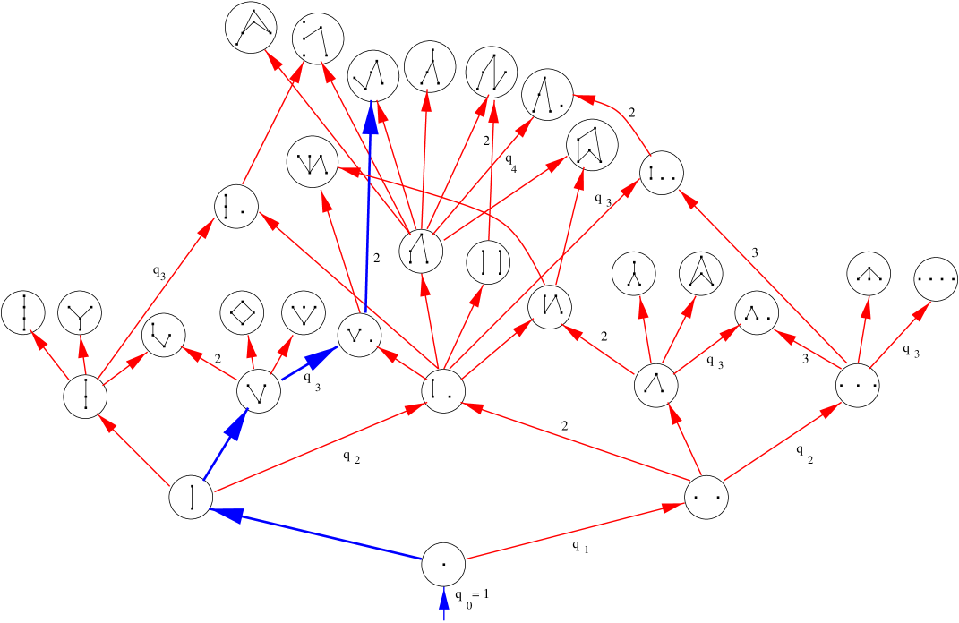
Figure 1: The poset of finite causets

The “decorations” on some of the transitions in figure 1 are for later use.) Any natural labeling of a causet $C\in{\cal P}$ determines uniquely a path in ${\cal P}$ beginning at the empty causet and ending at $C$. Conversely, any choice of upward path through this diagram determines a naturally labeled causet (or rather a set of them, since inequivalent labelings can sometimes give rise to the same path in ${\cal P}$.) We want the physics to be independent of labeling, so different paths in ${\cal P}$ leading to the same causet should be regarded as representing the same (partial) universe, the distinction between them being “pure gauge”.

The causal sets which can be formed by adjoining a single maximal element to a given causet will be called collectively a family. The causet from which they come is their parent, and they are siblings of each other. Each one is a child of the parent. The child formed by adjoining an element which is to the future of every element of the parent will be called the timid child. The child formed by adjoining an element which is spacelike to every other element will be called the gregarious child.

Each parent-child relationship in ${\cal P}$ describes a ‘transition’ $C\rightarrow{}C^{\prime}$, from one causal set to another induced by the birth of a new element. The past of the new element (a subset of $C$) will be referred to as the precursor set of the transition (or sometimes just the “precursor of the transition”). Normally, this precursor set is uniquely determined up to automorphism of the parent by the (isomorphism equivalence class of the) child, but (rather remarkably) this is not always the case. The symbol $\mathcal{C}_{n}$ will denote the set of causets with $n$ elements, and the set of all transitions from $\mathcal{C}_{n}$ to $\mathcal{C}_{n+1}$ will be called stage $n$.

As just remarked, each parent-child transition corresponds to a choice of partial stem in the parent (the precursor of the transition). Since there is a one-to-one correspondence between partial stems and antichains, a choice of child also corresponds to a choice of (possibly empty) antichain in the parent, the antichain in question being the set of maximal elements of the past of the new element. Note also that the new element will be linked to each element of this antichain.

1.2 Some examples

To help clarify the terminology introduced in the previous section, we give some examples. The 20 element causet of figure 2 was generated by the stochastic dynamics described herein, with the choice of parameters given by equation (16) below.

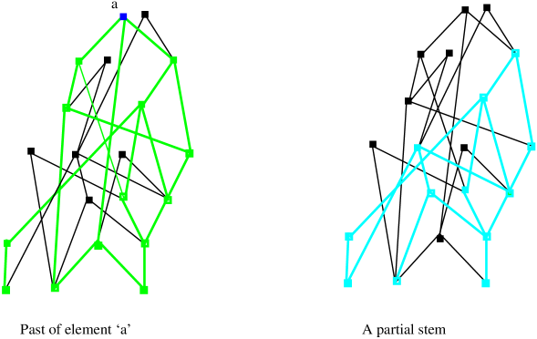
Figure 2: An example of a (‘typical’?) 20 element causal set

In the copy of this causet on the left, the past of element $a$ is highlighted. Notice that since we use the irreflexive convention for the order, $a$ is not included in its own past. In the the copy on the right, a partial stem of the causet is highlighted.

Figure 3 shows     and its children.

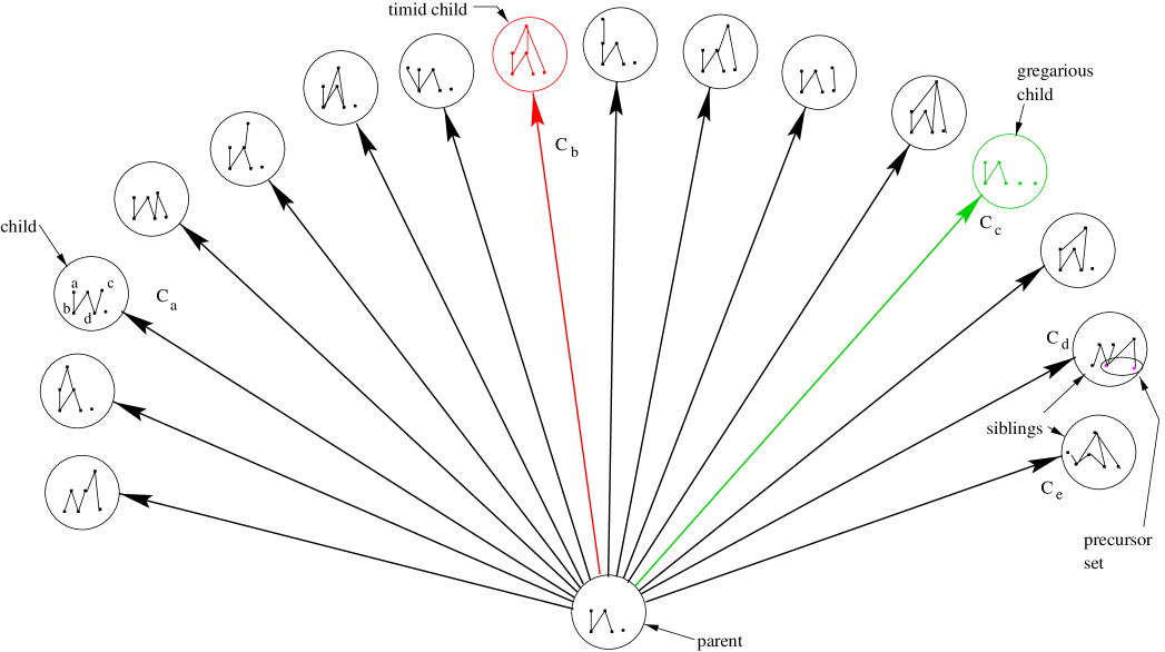
Figure 3: A family

The timid child is $C_{b}$ and the gregarious child is $C_{c}$. The precursor set leading to the transition to $C_{d}$ is shown in the ellipse. An example of an automorphism of $C_{a}$ is the map $a\leftrightarrow c,b\leftrightarrow d$ (the other elements remaining unchanged).

2 Transitive Percolation

In a sum over histories formulation of causal set theory, one might expect sums like

$$\sum_{\mathcal{C}}A(\mathcal{C},\{q\})$$ (1)

to be involved, where $A$ is a complex amplitude for the causal set $\mathcal{C}$, possibly depending on a set of parameters $\{q\}$. Kleitman and Rothschild have shown that the number of posets of cardinality $n$ grows faster than exponentially in $n$ and that asymptotically, almost every poset has a certain, almost trivial, “generic” form. (See [11].) Such a “generic poset” consists of three “tiers”, with $n/2$ elements in the middle tier and $n/4$ elements in the top and bottom tiers. For this reason, one might think that a sum like (1) would be dominated by causets which in no way resemble a spacetime, leading to a sort of “entropy catastrophe”. Nevertheless, it is not hard to forestall this catastrophe, and in fact the most naive choice of stochastic dynamics already does so. (Maybe this is not so different from the situation in ordinary quantum mechanics, where the smooth paths, which form a set of measure zero in the space of all paths, are the ones which dominate the sum over histories in the classical limit.)

The dynamics in question, which we will call “transitive percolation”, is perhaps the most obvious model of a randomly growing causet. It is an especially simple instance of a sequential growth dynamics, in which each new element forges a causal bond independently with each existing element with probability $p$, where $p\in[0,1]$ is a fixed parameter of the model. (Any causal relation implied by transitivity must then be added in as well.)

From a more static perspective, one can also describe transitive percolation by the following algorithm for generating a random poset:

1. Start with $n$ elements labeled $0,1,2,\cdots,n-1$   ($n=\infty$ is not excluded.)

2. With a fixed probability $p$, introduce a relation between every pair of points labeled $i$ and $j$, where $i<j$.

3. Form the transitive closure of these relations (e.g. if $2\prec 5$ and $5\prec 8$ then enforce that $2\prec 8$.)

Expressed in this manner, the model appears as a species of one dimensional directed percolation; hence the name we have given it (following D. Meyer).

From a physical point of view, transitive percolation has some appealing features, both as a model for a relatively small region of spacetime and as a cosmological model for spacetime as a whole. For $p\sim{1/n}$, there is a percolation transition, where the causet goes qualitatively from a large number of small disconnected universes for $p<p_{\mathrm{crit}}$ to a single connected universe for $p>p_{\mathrm{crit}}$. Moreover, computer simulations suggest strongly that the model possesses a continuum limit and exhibits scaling behavior in that limit with $p$ scaling roughly like $c\log{n}/n$ [12, 13]. The “cosmology” of transitive percolation is also suggestive — the universe cycles endlessly through phases of expansion, stasis, and contraction (via fluctuation) back down to a single element [14].

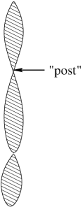
Figure 4: Transitive percolation cosmology

From all this, it is clear that the causets generated by transitive percolation do not at all resemble the 3-tier, generic causets of Kleitman and Rothschild, but rather they have the potential to reproduce a spacetime or a part of one. Nevertheless, the dynamics of transitive percolation is not viable as a theory of quantum gravity. One obvious reason is that it is stochastic only in the purely classical sense, lacking quantum interference. Another reason is that the future of any element of the causet is completely independent of anything “spacelike related” to that element. Therefore, the only spacetimes which a causal set generated by transitive percolation could hope to resemble would be homogeneous, such as the Minkowski or de Sitter spacetimes; but neither of these possibilities is compatible with the periodic re-collapses alluded to earlier. At best, therefore, one could hope to reproduce a small portion of such a homogeneous spacetime.

On the other hand, in computer simulations of transitive percolation [15], two independent (and coarse-graining invariant) dimension estimators have tended to agree with each other, one such estimator being that of [16] and the other being a simple “midpoint scaling dimension”. (Some other indicators of manifold-like behavior have tended to do much more poorly, but those are not invariant under coarse graining, whereas one would in any case expect to observe manifold like behavior only for a sufficiently coarse grained causal set.) In the pure percolation model, however, these dimension indicators vary with time (i.e. with $n$) and one must rescale $p$ if one wishes to hold the spacetime dimension constant. One may ask, then, if the model can be generalized by having $p$ vary with $n$ in an appropriate sense. We will see in the next section that something rather like this is in fact possible.

The transitive percolation model, incidentally, has attracted the interest of both mathematicians and physicists for reasons having nothing to do with quantum gravity. By physicists, it has been studied as a problem in the statistical mechanical field of percolation, as we have already alluded to. By mathematicians, it has been studied extensively as a branch of random graph theory (a poset being the same thing as a transitive acyclic directed graph). Some references on transitive percolation (viewed from whatever angle) are [11, 14, 17, 18, 15, 12, 13].

3 Physical requirements on the dynamics

As discussed in the previous section, one can think of transitive percolation as a sort of “birth process”, but as such, it is only one special case drawn from a much larger universe of possibilities. As preparation for describing these more general possible dynamical rules, let us consider the growth-sequence of a causal set universe.

First element ‘0’ appears (say with probability one, since the universe exists). Then element ‘1’ appears, either related to ‘0’ or not. Then element ‘2’ appears, either related to ‘0’ or ‘1’, or both, or neither. Of course if $1\succ 0$ and $2\succ 1$ then $2\succ 0$ by transitivity. Then element ‘3’ appears with some consistent set of ancestors, and so on and so forth. Because of transitivity, each new element ends up with a partial stem of the previous causet as its precursor set. The result of this process, obviously, is a naturally labeled causet (finite if we stop at some finite stage, or infinite if we do not) whose labels record the order of succession of the individual births. For illustration, consider the path in figure 1 delineated by the heavy arrows. Along this path, element ‘0’ appears initially, then element ‘1’ appears to the future of element ‘0’, then element ‘2’ appears to the future of element ‘0’, but not to the future of ‘1’, then element ‘3’ appears unrelated to any existing element, then element ‘4’ appears to the future of elements ‘0’, ‘1’ (say, or ‘2’, it doesn’t matter) and ‘3’, then element ‘5’ appears (not shown in the diagram), etc.

Let us emphasize once more that the labels 0, 1, 2, etc. are not supposed to be physically significant. Rather, the “external time” that they record is just a way to conceptualize the process, and any two birth sequences related to each other by a permutation of their labels are to be regarded as physically identical.

So far, we have been describing the kinematics of sequential growth. In order to define a dynamics for it, we may give, for each $n$-element causet $C$, the transition probability from it to each of its possible children. Equivalently, we give a transition probability for each partial stem within $C$. We wish to construct a general theory for these transition probabilities by subjecting them to certain natural conditions. In other words, we want to construct the most general (classically stochastic) “sequential growth dynamics” for causal sets. In stating the following conditions, we will employ the terminology introduced in the Introduction.

The condition of internal temporality

By this imposing sounding phrase, we mean simply that each element is born either to the future of, or unrelated to, all existing elements; that is, no element can arise to the past of an existing element.

We have already assumed this tacitly in describing what we mean by a sequential growth dynamics. An equivalent formulation is that the labeling induced by the order of birth must be natural, as defined above. The logic behind the requirement of internal temporality is that all physical time is that of the intrinsic order defining the causal set itself. For an element to be born to the past of another would be contradictory: it would mean that an event occurred “before” another which intrinsically preceded it.

The condition of discrete general covariance

As we have been emphasizing, the “external time” in which the causal set grows (equivalently the induced labeling of the resulting poset) is not meant to carry any physical information. We interpret this in the present context as being the condition that the net probability of forming any particular $n$-element causet $C$ is independent of the order of birth we attribute to its elements. Thus, if $\gamma$ is any path through the poset ${\cal P}$ of finite causal sets that originates at the empty causet and terminates at $C$, then the product of the transition probabilities along the links of $\gamma$ must be the same as for any other path arriving at $C$. (So general covariance in this setting is a type of path independence). We should recall here, however, that, as observed earlier, a link in ${\cal P}$ can sometimes represent more than one possible transition. Thus our statement of path-independence, to be technically correct, should say that the answer is the same no matter which transition (partial stem) we select to represent the link. Obviously, this immediately entails that all such representatives share the same transition probability.

We might with justice have required here conditions that are apparently much stronger, including the condition that any two paths through ${\cal P}$ with the same initial and final endpoints have the same product of transition probabilities. However, it is easy to see that this already follows from the condition stated. We therefore do not make it part of our definition of discrete general covariance, although we will be using it crucially.

Finally, it is well to remark here that just because the “arrival probability at $C$” is independent of path/labeling, that does not necessarily mean that it carries an invariant meaning. On the contrary a statement like “when the causet had 8 elements it was a chain” is itself meaningless before a certain birth order is chosen. This, also, is an aspect of the gauge problem, but not one that functions as a constraint on the transition probabilities that define our dynamics. Rather it limits the physically meaningful questions that we can ask of the dynamics. Technically, we expect that our dynamics (like any stochastic process) can be interpreted as a probability measure on a certain $\sigma$-algebra, and the requirement of general covariance will then serve to select the subalgebra of sets whose measures have direct physical meaning.

The Bell causality condition

The condition of “internal temporality” may be viewed as a very weak type of causality condition. The further causality condition we introduce now is quite strong, being similar to that from which one derives Bell’s inequalities. We believe that such a condition is appropriate for a classical theory, and we expect that some analog will be valid in the quantum case as well. (On the other hand, we would have to abandon Bell causality if our aim were to reproduce quantum effects from a classical stochastic dynamics, as is sometimes advocated in the context of “hidden variable theories”. Given the inherent non-locality of causal sets, there is no logical reason why such an attempt would have to fail.)

The physical idea behind our condition is that events occurring in some part of a causal set $C$ should be influenced only by the portion of $C$ lying to their past. In this way, the order relation constituting $C$ will be causal in the dynamical sense, and not only in name. In terms of our sequential growth dynamics, we make this precise as the requirement that the ratio of the transition probabilities leading to two possible children of a given causet depend only on the triad consisting of the two corresponding precursor sets and their union.

Thus, let $C\rightarrow{}C_{1}$ designate a transition from $C\in\mathcal{C}_{n}$ to $C_{1}\in\mathcal{C}_{n+1}$, and similarly for $C\rightarrow{}C_{2}$. Then, the Bell causality condition can be expressed as the equality of two ratios:

$$\frac{prob(C\rightarrow C_{1})}{prob(C\rightarrow C_{2})}=\frac{prob(B\rightarrow B_{1})}{prob(B\rightarrow B_{2})}$$ (2)

where $B\in\mathcal{C}_{m}$, ${m}\leq{n}$, is the union of the precursor set of $C\rightarrow C_{1}$ with the precursor set of $C\rightarrow C_{2}$, $B_{1}\in\mathcal{C}_{m+1}$ is $B$ with an element added in the same manner as in the transition $C\rightarrow{C_{1}}$, and $B_{2}\in\mathcal{C}_{m+1}$ is $B$ with an element added in the same manner as in the transition $C\rightarrow C_{2}$. (Notice that if the union of the precursor sets is the entire parent causet, then the Bell causality condition reduces to a trivial identity.)

To clarify the relationships among the causets involved, it may help to characterize the latter in yet another way. Let $e_{1}$ be the element born in the transition $C\rightarrow{}C_{1}$ and let $e_{2}$ be the element born in the transition $C\rightarrow{}C_{2}$. Then $C_{i}=C\cup\{e_{i}\}$ ($i=1,2$), and we have $B=(\mathrm{past}\,e_{1})\cup(\mathrm{past}\,e_{2})$ and $B_{i}=B\cup\{e_{i}\}$ ($i=1,2$).

By its definition, Bell causality relates ratios of transition probabilities belonging to one “stage” of the growth process to ratios of transition probabilities belonging to previous stages. For illustration, consider the case depicted in figure 5.

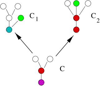
Figure 5: Illustrating Bell causality

The precursor $P_{1}$ of the transition $C\rightarrow{}C_{1}$ contains only the earliest (minimum) element of $C$, shown in the figure as a pattern-filled dot. The precursor $P_{2}$ of $C\rightarrow{}C_{2}$ contains as well the next earliest element, shown as a (different pattern)-filled dot. The union of the two precursors is thus $B={P_{1}}\cup{P_{2}}=P_{2}$. The elements of $C$ depicted as open dots belong to neither precursor. Such elements will be called spectators. Bell causality says that the spectators can be deleted without affecting relative probabilities. Thus the ratio of the transition probabilities of figure 5 is equal to that of figure 6.

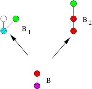
Figure 6: Illustrating Bell causality - spectators do not affect relative probability

The Markov sum rule

As with any Markov process, we must require that the sum of the full set of transition probabilities issuing from a given causet be unity. However, the set we have to sum over depends in a subtle manner on the extent to which we regard causal set elements as “distinguishable”. Heretofore we have identified distinct transitions with distinct precursor sets of the parent. In doing so, we have in effect been treating causet elements as distinguishable (by not identifying with each other, precursor sets related by automorphisms of the parent), and this is what we shall continue to do. Indeed, this is the counting of children used implicitly by transitive percolation, so we keep it here for consistency. With respect to the diagram of figure 1, this method of counting has the effect of introducing coefficients into the sum rule, equal to the number of partial stems of the parent which could be the precursor set of the transition. For the transitions depicted there, these coefficients (when not one) are shown next to the corresponding arrow.

We remark here that these sum-rule coefficients admit an alternative description in terms of embeddings of the parent into the child (as a partial stem). Instead of saying “the number of partial stems of the parent which could be the past of the new element”, we could say “the number of order preserving injective maps from the parent onto partial stems of the child, divided by the number of automorphisms of the child”. (The proof of this equivalence will appear in [19].)

4 The general form of the transition probabilities

We seek to derive a general prescription which gives, consistent with our requirements, the transition probability from an element of $\mathcal{C}_{n}$ to an element of $\mathcal{C}_{n+1}$. To avoid having to deal with special cases, we will assume throughout that no transition probability vanishes. Thus the solution we find may be termed “generic”, but not absolutely general.

In this connection, we want to point out that one probably does not obtain every possible solution of our conditions by taking limits of the generic solution, and the special theories which result from taking certain transition probabilities to vanish must be treated separately. One such special theory is the originary percolation model, which is the same as the transitive percolation model, but with the added restriction that each element except the original one must have at least one ancestor among the previous elements. The net effect is that the growing causal set is required to have an “origin” (= unique minimum element) at all stages. (Generalizations are also possible in which a more complex full stem of the causet is enforced.) The poset of originary causets can be transformed into the poset of all causets (exactly) by removing the origin from every originary causet. The transition probabilities for originary percolation are just those of ordinary transitive percolation with an added factor of $(1-q^{n})$ in the denominator at stage $n$.

4.1 Counting the free parameters

A theory of the sort we are seeking provides a probability for each transition, so without further restriction, it would contain a free parameter for every possible antichain of every possible (finite) causet. We will see, however, that the requirements described above in Section 3 drastically limit this freedom.

Lemma 1

There is at most one free parameter per family.

Proof: Consider a parent and its children. Every such child, except the timid child, participates in a Bell causality equation with the gregarious child. (See the proof of Lemma 5 in the Appendix.) Hence (since Bell causality equates ratios), all these transitions are determined up to an overall factor. This leaves two free parameters for the family. The Markov sum rule gives another equation, which exhausts itself in determining the probability of the timid child. Hence precisely one free parameter per family remains after Bell Causality and the sum rule are imposed. $\Box$

Lemma 2

The probability to add a completely disconnected element (the “gregarious child transition”) depends only on the cardinality of the parent causal set.

Proof:

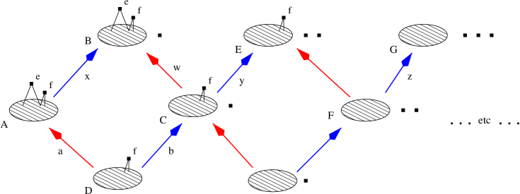
Figure 7: Equality of “gregarious child” transitions

Consider an arbitrary causet $A$, with a maximal element $e$, as indicated in figure 7. Adjoining a disconnected element to $A$ produces the causet $B$. Then, removing $e$ from $B$ leads to the causet $C$, which can be looked upon as the gregarious child of the causet $D=A\backslash\{e\}$. Adding another disconnected element to $C$ leads to a causet $E$ with (at least) two completely disconnected elements. Now, by general covariance,

$$ax=bw$$

and by Bell causality,

$$\frac{y}{w}=\frac{b}{a}$$

(the disconnected element in $C$ acts as the spectator here). Thus

$$ax=bw=ay\Longrightarrow x=y$$

(Recall that we have assumed that no transition probability vanishes.) Repeating our deductions with $C$ in the place of $A$ in the above argument (and a new maximal element $f$ in the place of $e$), we see that $y=z$, where $z$ is the probability for the transition from $F$ to $G$ as shown. Continuing in this way until we reach the antichain $A_{n}$ shows finally that $x=q_{n}$, where we define $q_{n}$ as the transition probability from the $n$-antichain to the ($n+1$)-antichain. Since our starting causet $A$ was not chosen specially, this completes the proof. $\;\;\Box$

If our causal sets are regarded as entire universes, then a gregarious child transition corresponds to the spawning of a new, completely disconnected universe (which is not to say that this new universe will not connect up with the existing universe in the future). Lemma 2 proves that the probability for this to occur does not depend on the internal structure of the existing universe, but only on its size, which seems eminently reasonable. In the sequel, we will call this probability $q_{n}$.

With Lemmas 1 and 2, we have reduced the number of free parameters (since every family has a gregarious child) to 1 per stage, or what is the same thing, to one per causal set element. In the next sections we will see that no further reduction is possible based on our stated conditions. Thus, the transition probabilities $q_{n}$ can be identified as the free parameters or “coupling constants” of the theory. They are, however, restricted further by inequalities that we will derive below.

4.2 The general transition probability in closed form

Given the $q_{n}$, the remaining transition probabilities (for the non-gregarious children) are determined by Bell causality and the sum rule, as we have seen. Here we derive an expression in closed form for an arbitrary transition probability in terms of causet invariants and the parameters $q_{n}$.

Mathematical form of transition probabilities

We use the following notation:

$\alpha_{n}$	an arbitrary transition probability from $\mathcal{C}_{n}$ to $\mathcal{C}_{n+1}$
$\beta_{n}$	a transition whose precursor set is not the entire parent (‘non-timid’ transition)
$\gamma_{n}$	a transition whose precursor set is the entire parent (‘timid’ transition)

Notice that the subscript $n$ here refers only to the number of elements of the parent causet; it does not exhibit which particular transition of stage $n$ is intended. A more complete notation might provide $\alpha$, $\beta$ and $\gamma$ with further indices to specify both the parent causet and the precursor set within the parent.

We also set $q_{0}\equiv{}1$ by convention.

Lemma 3

Each transition probability $\alpha_{n}$ of stage $n$ has the form

$$q_{n}\sum_{i=0}^{n}{\lambda_{i}\frac{1}{q_{i}}}$$ (3)

where the $\lambda_{i}$ are integers depending on the individual transition in question.

Proof: This is easily seen to be true for stages 0 and 1. Assume it is true for stage $n-1$. Consider a non-timid transition probability $\beta_{n}$ of stage $n$. Bell causality gives

$$\frac{\beta_{n}}{q_{n}}=\frac{\alpha_{n-1}}{q_{n-1}}$$

where $\alpha_{n-1}$ is an appropriate transition probability from stage $n-1$. So by induction

$$\beta_{n}=\alpha_{n-1}\frac{q_{n}}{q_{n-1}}=\sum_{i=0}^{n-1}\lambda_{i}\frac{q_{n-1}}{q_{i}}\frac{q_{n}}{q_{n-1}}=\sum_{i=0}^{n-1}\lambda_{i}\frac{q_{n}}{q_{i}}.$$ (4)

For a timid transition probability $\gamma_{n}$, we use the Markov sum rule:

$$\gamma_{n}=1-\sum_{j}\beta_{nj}$$ (5)

where $j$ labels the possible non-timid transitions (i.e. the set of proper partial stems of the parent). But then, substituting (4) yields immediately

$$\gamma_{n}=1-\sum\limits_{j}\sum\limits_{i=0}^{n-1}{\lambda_{ji}\over q_{i}}q_{n}=1-\sum\limits_{i=0}^{n-1}{\sum_{j}\lambda_{ji}\over q_{i}}q_{n}\,,$$

which we clearly can put into the form (3) by taking $\lambda_{i}=-\sum_{j}\lambda_{ji}$ for $i<n$ and $\lambda_{n}=1$. $\Box$

Another look at transitive percolation

The transitive percolation model we described earlier is consistent with the four conditions of Section 3. To see this, consider an arbitrary causal set $C_{n}$ of size $n$. The transition probability $\alpha_{n}$ from $C_{n}$ to a specified causet $C_{n+1}$ of size $n+1$ is given by

$$\alpha_{n}=p^{m}(1-p)^{n-\varpi}$$ (6)

where $m$ is the number of maximal elements in the precursor set and $\varpi$ is the size of the entire precursor set. (This becomes clear if one recalls how the precursor set of a newborn element is generated in transitive percolation: first a set of ancestors is selected at random, and then the ancestors implied by transitivity are added. From this, it follows immediately that a given stem $S\subseteq{}C_{n}$ results from the procedure iff (i) every maximal element of $S$ is selected in the first step, and (ii) no element of $C_{n}\backslash{}S$ is selected in the first step.) In particular, we see that the “gregarious transition” will occur with probability $q_{n}=q^{n}$, where $q=1-p$.

Now consider our four conditions. Internal temporality was built in from the outset, as we know. Discrete general covariance is seen to hold upon writing the net probability of a given $C_{n}$ explicitly in terms of causet invariants (writing it in “manifestly covariant form”) as

$$P(C_{n})=Wp^{L}q^{{n\choose 2}-R}$$

where $L$ is the number of links in $C_{n}$, $R$ the number of relations, and $W$ the number of (natural) labelings of $C_{n}$.

To see that transitive percolation obeys Bell causality, consider an arbitrary parent causet. The transition probability to a given child is exhibited in eq. (6). Consider two different children, one with $(m,\varpi)$=($m_{1}$,$\varpi_{1}$) and the other with $(m,\varpi)$=($m_{2}$,$\varpi_{2}$). Bell causality requires that the ratio of their transition probabilities be the same as if the parent were reduced to the union of the precursor sets of the two transitions, i.e. it requires

$$\frac{p^{m_{1}}q^{n-\varpi_{1}}}{p^{m_{2}}q^{n-\varpi_{2}}}=\frac{p^{m_{1}}q^{n^{\prime}-\varpi_{1}}}{p^{m_{2}}q^{n^{\prime}-\varpi_{2}}}$$

where $n^{\prime}$ is the cardinality of the union of the precursor sets of the two transitions. Thus, Bell causality is satisfied by inspection.

Finally, the Markov sum rule is essentially trivial. At each stage of the growth process, a preliminary choice of ancestors is made by a well-defined probabilistic procedure, and each such choice is mapped uniquely onto a choice of partial stem. Thus the induced probabilities of the partial stems sum automatically to unity.

The general transition probability

In the previous section we have shown that transitive percolation produces transition probabilities (6) consistent with all our conditions. By equating the right hand side of (6) to the general form (3) of Lemma 3, we can solve for the $\lambda_{i}$ and thus obtain the general solution of our conditions:

$$\alpha_{n}=\sum_{i=0}^{n}{\lambda_{i}\frac{1}{q_{i}}}\,q_{n}=p^{m}(1-p)^{n-\varpi}=(1-q)^{m}q^{n-\varpi}$$

Expanding the factor $(1-q)^{m}$, and using the fact that $q_{n}=q^{n}$ for transitive percolation, we get

$$\lambda_{i}=(-)^{\varpi-i}{m\choose\varpi-i}.$$

So an arbitrary transition probability in the general dynamics is, according to (3)

$$\alpha_{n}=\sum_{i=0}^{n}(-)^{\varpi-i}{m\choose\varpi-i}\frac{q_{n}}{q_{i}}.$$

Noting that the binomial coefficients are zero for $\varpi-i\notin\{0..m\}$, and rearranging the indices, we obtain

$$\alpha_{n}=\sum_{k=0}^{m}(-)^{k}{m\choose k}\frac{q_{n}}{q_{\varpi-k}}$$ . (7)

This form for the transition probability exhibits its causal nature particularly clearly: except for the overall normalization factor $q_{n}$, $\alpha_{n}$ depends only on invariants of the associated precursor set.

4.3 Inequalities

Since the $\alpha_{n}$ are classical probabilities, each must lie between 0 and 1, and this in turn restricts the possible values of the $q_{n}$. Here we show that it suffices to impose only one inequality per stage; all the others (two per child) then follow. More precisely, what we show is that, if $q_{n}>0$ for all $n$, and if $\alpha_{n}\geq{0}$ for the “timid” transition from the $n$-antichain, then all the $\alpha_{n}$ lie in $[0,1]$. This we establish in the following two “Claims”.
Claim   In order that all the transition probabilities $\alpha_{n}$ fall between 0 and 1, it suffices that each timid transition probability be $\geq 0$.
Proof: As described in the proofs of lemmas 1 and 5, each non-timid transition (of stage $n$) is given (via Bell causality) by

$$\alpha_{n}=\alpha_{m}\frac{q_{n}}{q_{m}}$$

where $m$ is some natural number less than $n$. The $q$’s are positive. So if the probabilities of the previous stages are positive, then the non-timid probabilities of stage $n$ are also positive. It follows by induction that all but the timid transition probabilities are positive (since $\alpha_{0}=q_{0}=1$ obviously is). But for the timid transition of each family, we have

$$\gamma_{n}=1-\sum_{i}\beta_{i}$$ (8)

where each $\beta_{i}$ is positive. If any of the $\beta_{i}$ is greater than one, $\gamma_{n}$ will obviously be negative. Also (8) plainly cannot be greater than one. Consequently, if we require that $\gamma_{n}$ be positive, then all transition probabilities in the family will be in $[0,1]$. $\Box$

In a timid transition, the entire parent is the precursor set, so $\varpi=n$. The inequalities constraining each probability of a given family to be in $[0,1]$ therefore reduce to the sole condition

$$\sum_{k=0}^{m}(-)^{k}{m\choose k}\frac{1}{q_{n-k}}\geq 0\,.$$ (9)

Claim   The most restrictive inequality of stage $n$ is the one arising from the $n$-antichain, i.e. the one for which $m=n$. All other inequalities of stage $n$ follow from this inequality and the inequalities for smaller $n$.

Proof: Assume that we have, for $m=n$,

$$\sum_{k=0}^{n}(-)^{k}{n\choose k}\frac{1}{q_{n-k}}\geq 0.$$

Add to this the inequality from stage $n-1$,

$$\sum_{k=0}^{n-1}(-)^{k}{n-1\choose k}\frac{1}{q_{n-k-1}}=\sum_{k=0}^{n}(-)^{k-1}{n-1\choose k-1}\frac{1}{q_{n-k}}\geq 0$$

to get

$$\sum_{k=0}^{n-1}(-)^{k}{n-1\choose k}\frac{1}{q_{n-k}}\geq 0.$$

This is the inequality of stage $n$ for $m=n-1$. (We have used the identity ${n\choose k}={n-1\choose k}+{n-1\choose k-1}$.) Adding to it the inequality of stage $n-1$ with $m=n-2$ yields the inequality of stage $n$ for $m=n-2$. Repeating this process will give all the inequalities of stage $n$. $\;\;\Box$

It is helpful to introduce the quantities

$$t_{n}=\sum_{k=0}^{n}(-)^{n-k}{n\choose k}\frac{1}{q_{k}}$$ (10)

Obviously, we have $t_{0}=1$ (since $q_{0}=1$), and we have seen that the full set of inequalities restricting the $q_{n}$ will be satisfied iff $t_{n}\geq 0$ for all $n$. (Recall we are assuming $q_{n}>0,\,\forall n$.) Moreover, given the $t_{n}$, we can recover the $q_{n}$ by inverting (10):

Lemma 4

$$\frac{1}{q_{n}}=\sum_{k=0}^{n}{n\choose k}t_{k}$$ (11)

Proof: This follows immediately from the identity

$$\sum\limits_{k=0}^{n}{n\choose k}(-)^{n-k}{k\choose m}=\delta^{n}_{m}\qquad\qquad\qquad\Box$$

Thus, the $t_{n}$ may be treated as free parameters (subject only to $t_{n}\geq{}0$ and $t_{0}=1$), and the $q_{n}$ can then be derived from (11). If this is done, the remaining transition probabilities $\alpha_{n}$ can be re-expressed more simply in terms of the $t_{n}$ by inserting (11) into (7) to get

$$\frac{\alpha_{n}}{q_{n}}=\sum_{l}t_{l}\sum_{k}(-)^{k}{m\choose k}{\varpi-k\choose l}=\sum_{l}t_{l}{\varpi-m\choose\varpi-l}$$

whence

$$\alpha_{n}=\frac{\sum_{l=m}^{\varpi}{\varpi-m\choose\varpi-l}t_{l}}{\sum_{j=0}^{n}{n\choose j}t_{j}}$$ (12)

Here, we have used an identity for binomial coefficients that can be found on page 63 of [20].

In this way, we arrive at the general solution of our inequalities. (Actually, we go slightly beyond our “genericity” assumption that $\alpha_{n}\not=0$ if we allow some of the $t_{n}$ to vanish; but no harm is done thereby.)

Let us conclude this section by noting that (11) implies

$$q_{0}\equiv 1\geq q_{1}\geq q_{2}\geq q_{3}\geq\cdots$$ (13)

If we think of the $q_{n}$ as the basic parameters or “coupling constants” of our sequential growth dynamics, then it is as if the universe had a free choice of one parameter at each stage of the process. We thus get an “evolving dynamical law”, but the evolution is not absolutely free, since the allowable values of $q_{n}$ at every stage are limited by the choices already made. On the other hand, if we think of the $t_{n}$ as the basic parameters, then the free choice is unencumbered at each stage. However, unlike the $q_{n}$, the $t_{n}$ cannot be identified with any dynamical transition probability. Rather, they can be realized as ratios of two such probabilities, namely as the ratio $x_{n}/q_{n}$, where $x_{n}$ is the transition probability from an antichain of $n$ elements to the timid child of that antichain. (Thus, if we suppose that the evolving causet at the beginning of stage $n$ is an antichain, then $t_{n}$ is the probability that the next element will be born to the future of every element, divided by the probability that the next element will be born to the future of no element.)

4.4 Proof that this dynamics obeys the physical requirements

To complete our derivation, we must show that the sequential growth dynamics given by (7) or (12) obeys the four conditions set out in section 3.

Internal temporality

This condition is built into our definition of the growth process.

Discrete general covariance

We have to show that the product of the transition probabilities $\alpha_{n}$ associated with a labeling of a fixed finite causet $C$ is independent of the labeling. But this follows immediately from (7) [or (12)] once we notice that what remains after the overall product

$$\prod\limits_{j=0}^{|C|-1}q_{j}$$

is factored out, is a product over all elements $x\in{C}$ of poset invariants depending only on the structure of $\mathrm{past}(x)$.

Bell causality

Bell causality states that the ratio of the transition probabilities for two siblings depends only on the union of their precursors. Looking at (7), consider the ratio of two such probabilities $\alpha_{n1}$ and $\alpha_{n2}$. The $q_{n}$ factors will cancel, leading to an expression which depends only on $\varpi_{1}$, $\varpi_{2}$, $m_{1}$, and $m_{2}$. Since these are all determined by the structure of the precursor sets, Bell causality is satisfied.

Markov sum rule

The sum rule states that the sum of all transition probabilities $\alpha_{n}$ from a given parent $C$ (of cardinality $|C|=n$) is unity. Since a child can be identified with a partial stem of the parent, we can write this condition, in view of (12), as

$$\sum_{S}\sum_{l}t_{l}{|S|-m(S)\choose l-m(S)}=\sum_{j}t_{j}{n\choose j}$$ (14)

where $S$ ranges over the partial stems of $C$. This must hold for any $t_{l}$, since they may be chosen freely. Reordering the sums and equating like terms yields

$$\forall l,\ \sum_{S}{|S|-m(S)\choose l-m(S)}={n\choose l}\,,$$ (15)

an infinite set of identities which must hold if the sum rule is to be satisfied by our dynamics.

The simplest way to see that (15) is true is to resort to transitive percolation, for which $t_{l}=t^{l}$, where $t=p/q=p/(1-p)$. In that case we know that the sum rule is satisfied, so by inspection of (14), we see that the identity (15) must be true.

A more intuitive proof is illustrated well by the case of $l=3$. Group the terms on the left side according to the number of maximal elements:

$$\begin{array}[]{ccccccccr}\sum\limits_{S\,|\,m(S)=0}{|S|-0\choose 3-0}&+&\sum\limits_{S\,|\,m(S)=1}{|S|-1\choose 3-1}&+&\sum\limits_{S\,|\,m(S)=2}{|S|-2\choose 3-2}&+&\sum\limits_{S\,|\,m(S)=3}{|S|-3\choose 3-3}&=&{n\choose 3}\\ 0&+&\sum\limits_{S\,|\,m(S)=1}{|S|-1\choose 2}&+&\sum\limits_{S\,|\,m(S)=2}(|S|-2)&+&\sum\limits_{S\,|\,m(S)=3}1&=&{n\choose 3}\end{array}$$

The first term is zero because the only partial stem with zero maximal elements is empty (i.e. $|S|=0$). The second term is a sum over all partial stems with one maximal element. This is equivalent to a sum over elements, with the element’s inclusive past forming the partial stem. The summand chooses every possible pair of elements to the past of the maximal element. Thus the second term overall counts the 3-element subcausets of $C$ with a single maximal element. There are two possibilities here, the three-chain     and the “lambda”    . The third term sums over partial stems with two maximal elements, which is equivalent to summing over 2 element antichains, the inclusive past of the antichain being the partial stem. The summand then counts the number of elements to the past of the two maximal ones. Thus the third term overall counts the number of three element subcausets with precisely two maximal elements. Again there are two possibilities, the “V”    , and the “L”,    . Finally, the fourth term is a sum over partial stems with three maximal elements, and this can be interpreted as a sum over all three element antichains    . As this example illustrates, then, the left hand side of (15) counts the number of $l$ element subcausets of $C$, placing them into “bins” according to the number of maximal elements of the subcauset. Adding together the bin sizes yields the total number of $l$ element subsets of $C$, which of course equals ${n\choose l}$.

4.5 Sample cosmologies

The physical consequences of differing choices of the $t_{n}$ remain to be explored. To get an initial feel for this question, we list some simple examples. (Recall our convention that $t_{0}=1$, or equivalently, $q_{0}=1$, where $q_{0}$ is the probability that the universe is born at all.)

• “Dust universe”

  $$t_{0}=1,\ t_{i}=0,\;i\geq 1$$

  This universe is simply an antichain, since, according to (11), $q_{n}=1$ for all $n$.

• “Forest universe”

  $$t_{0}=t_{1}=1;\;t_{i}=0,\;i\geq 2$$

  This yields a universe consisting wholly of trees, since (see the next example) $t_{2}=t_{3}=t_{4}=\cdots=0$ implies that no element of the causet can have more than one past link. The particular choice of $t_{1}=1$ has in addition the remarkable property that, as follows easily from (12), every allowed transition of stage $n$ has the same probability $1/(n+1)$.

• Case of limited number of past links

  $$t_{i}=0,\;i>n_{0}$$

  Referring to expression (12) one sees at once that $\alpha_{n}$ vanishes if $m>n_{0}$. Hence, no element can be born with more than $n_{0}$ past links or “parents”. This means in particular that any realistic choice of parameters will have $t_{n}>0$ for all $n$, since an element of a causal set faithfully embeddable in Minkowski space would have an infinite number of past links.

• Transitive percolation

  $$t_{n}=t^{n}$$

  We have seen that for transitive percolation, $q_{n}=q^{n}$, where $q=1-p$. Using the binomial theorem, it is easy to learn from (11) or (10) that this choice of $q_{n}$ corresponds to $t_{n}=t^{n}$ with $t=p/q$. Clearly, $t$ runs from 0 to $\infty$ as $p$ runs from 0 to 1.

• A more lifelike choice?

  $$t_{n}=\frac{1}{n!}$$ (16)

  We have seen that transitive percolation with constant $p$ yields causets which could reproduce — at best — only limited portions of Minkowski space. To do any better, one would have to scale $p$ so that it decreased with increasing $n$ [12, 13, 15]. This suggests that $t_{n}$ should fall off faster than in any percolation model, hence (by the last example) faster than exponentially in $n$. Obviously, there are many possibilities of this sort (e.g. $t_{n}\sim{}e^{-\alpha{}n^{2}}$), but one of the simplest is $t_{n}\sim{c}/n!$  This would be our candidate of the moment for a physically most realistic choice of parameters.

5 The stochastic growth process as such

We have seen that, associated with every labeled causet $\widetilde{C}$ of size $N$, is a net “probability of formation” $P(\widetilde{C})$ which is the product of the transition probabilities $\alpha_{i}$ of the individual births described by the labeling:

$$P(\widetilde{C})=\prod\limits_{i=0}^{N-1}\alpha_{i}$$

where $\alpha_{i}=\alpha(i,\varpi_{i},m_{i})$ is given by (7) or (12). We have also seen that $P$ is in fact independent of the labeling and may be written as $P(C)$ where $C$ is the unlabeled causet corresponding to $\widetilde{C}$. To bring this out more clearly, let us define

$$\lambda(\varpi,m)=\sum\limits_{k=m}^{\varpi}{\varpi-m\choose\varpi-k}t_{k}$$ (17)

Then $q_{i}=\lambda(i,0)^{-1}$ and we have

$$\alpha_{i}(i,\varpi_{i},m_{i})={\lambda(\varpi_{i},m_{i})\over\lambda(i,0)}\,,$$

whence $P(\widetilde{C})=\prod\limits_{i=0}^{N-1}\lambda(\varpi_{i},m_{i})/\prod\limits_{j=0}^{N-1}\lambda(j,0)$, or expressed more intrinsically,

$$P(C)={\prod\limits_{x\in C}\lambda(\varpi(x),m(x))\over\prod\limits_{j=0}^{|C|-1}\lambda(j,0)}\,,$$ (18)

where $\varpi(x)=|\mathrm{past}{x}|$ and $m(x)=|{\rm maximal}(\mathrm{past}x)|$. This expression, as far as it goes, is manifestly “causal” and “covariant” in the senses explained above. As also explained above, however, it has no direct physical meaning. Here we briefly discuss some probabilities which do have a fully covariant meaning and show how, in simple cases, they are related to $N\rightarrow\infty$ limits of probabilities like (18).

First, let us notice that the net probability of arriving at a particular $C\in{\cal P}$ is not $P(C)$ but

$${\rm Prob}_{N}(C)=W(C)\,P(C)$$

where $N=|C|$ and $W(C)$ is the number of inequivalent labelings of $C$, or in other words, the total number of paths through ${\cal P}$ that arrive at $C$, each link being taken with its proper multiplicity.

Now as a rudimentary example of a truly covariant question, let us take “Does the two-chain ever occur as a partial stem of $C$?”. The answer to this question will be a probability, $P$, which it is natural to identify as

$$P=\lim_{N\rightarrow\infty}{\rm Prob}_{N}(X_{N})\,,$$

where $X_{N}$ is the event that “at stage $N$”, $C$ possesses a partial stem which is a two-chain. In this connection, we conjecture that the questions of the form “Does $P$ occur as a partial stem of $C$?” furnish a physically complete set, when $P$ ranges over all (isomorphism equivalence classes of) finite causets.

6 Two Ising-like state-models

In this section, we present two Ising-like state-models from which $P(C)$ of equation (18) can be obtained. In the main we just indicate the results, leaving the details to appear elsewhere [19]. The two models come from taking (7) or, respectively, (12) as the starting point. In each case, the idea is to interpret the binomial coefficients which occur in these formulas as describing a sum over subsets of relations of $C$. If we work with (7) these will be subsets of the set of links of $C$; if we work with (12) they will be subsets of the set of relations of $C$ that are not links.

Let us take first equation (7). Reinterpreting the binomial coefficients in the manner indicated, and proceeding as in the derivation of (18), we arrive at an expression for $P(C)$ in terms of a sum over $\hbox{\openface Z}_{2}$-valued “spins” $\sigma$ living on the relations of $C$. In summing over configurations, however, the spins $\sigma$ on the non-link relations are set permanently to 1; only those on the links vary. With $\sigma=1$ interpreted as “presence” and $\sigma=0$ as “absence”, the contribution of a particular spin configuration $\sigma$ is an overall sign times the product of one “vertex factor” for each $x\in{C}$. The vertex factor is $q_{r}^{-1}$, where $r$ is the number of present relations having $x$ as future endpoint, and the sign is $(-)^{a}$, where $a$ is the number of absent relations. (In addition, there is a constant overall factor in $P(C)$ of $\prod_{j=0}^{|C|-1}q_{j}$.)

In the second state model, we begin with (12), or better (18) itself, and proceed similarly. The result is again a sum over spins $\sigma$ residing on the relations, this time with all the terms being positive (as is required of physical Boltzmann weights). In this second model, the spins on the links are set permanently to 1 while those on the non-links vary. The “vertex factor” coming from $x\in{C}$ now is $t_{r}$, where $r$ is again the number of relations present and “pointing to $x$”.

These two models (and especially the second) show that our sequential growth dynamics can be viewed as a form of “induced gravity” obtained by summing over (“integrating out”) the values of our underlying spin variables $\sigma$. This underlying “matter” theory may or may not be physically reasonable (Does it obey its own version of Bell causality, for example? Is it local in an appropriate sense?), but at a minimum, it serves to illustrate how a theory of non-gravitational matter can be hidden within a theory that one might think to be limited to gravity alone.

7 Further Work

Our dynamics can be simulated; for $t_{n}=1/n!$ it takes a minute or so to generate a 64 element causet on a DEC Alpha 600 workstation. Analytic results, so far, are available only for the special case of transitive percolation. An important question, of course, is whether some choice of the $t_{n}$ can reproduce general relativity, or at least reproduce a Lorentzian manifold for some range of $t$’s and of $n=|C|$. Similarly, one can ask whether our “Ising matter” gives rise to an interesting effective field theory and what relation it has with the local scalar matter on a background causal set studied in [25, 26]?

Another set of questions concerns the possibility of a more “manifestly covariant” formulation of our sequential growth dynamics – or of more general forms of causal set dynamics. Can Bell causality be formulated in a gauge invariant manner, without reference to a choice of birth sequence? Is our conjecture correct that all meaningful assertions are logical combinations of assertions about the occurrence of partial stems (“past sets”)? (Such questions seem likely to arise with special urgency in any attempt to generalize our dynamics to the quantum case.)

Also, there are the special cases we left unstudied. There exist originary analogs of all of our dynamics, for example. Are there other special, non-generic cases of interest?

We might continue multiplying questions, but let’s finish with the question of how to discover a quantum generalization of our dynamics. Since our theory is formulated as a type of Markov process, and since a Markov process mathematically is a probability measure on a suitable sample space, the natural quantum generalization would seem to be a quantum measure[1] (or equivalent “decoherence functional”) on the same sample space. The question then would be whether one could find appropriate quantum analogs of Bell causality and general covariance formulated in terms of such a quantum measure. If so, we could hope that, just as in the classical case treated herein, these two principles would lead us to a relatively unique quantum causet dynamics, or rather to a family of them among which a potential quantum theory of gravity would be recognizable.

It is a pleasure to thank Avner Ash for a stimulating discussion at a critical stage of our work. The research reported here was supported in part by NSF grant PHY-9600620 and by a grant from the Office of Research and Computing of Syracuse University.

Appendix: Consistency of the conditions

Our analysis of the conditions of Bell causality et al. unfolded in the form of several lemmas. Here we present some similar lemmas which strictly speaking are not needed in the present context, but which further elucidate the relationships among our conditions. We expect these lemmas can be useful in any attempt to formulate generalizations of our scheme, in particular quantal generalizations.

Lemma 5

The Bell causality equations are mutually consistent.

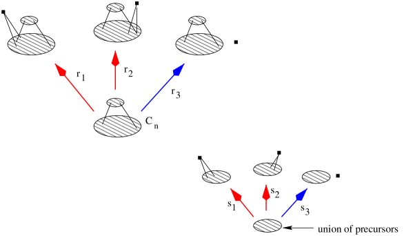
Figure 8: two families related by Bell causality

Proof: The top of figure 8 shows three children of an arbitrary causal set $C_{n}$. The shaded ellipses represent portions of $C_{n}$. The small square indicates the new element whose birth transforms $C_{n}$ into a causal set $C_{n+1}$ of the next stage. The smaller ellipse “stacked on top of” the larger ellipse represents a subcauset of $C_{n}$ which does not intersect the precursor set of any of the transitions being considered (i.e. none of its elements lie to the past of any of the new elements). This small ellipse thus consists entirely of “spectators” to the transitions under consideration. The bottom part of figure 8 shows the corresponding parent and children when these spectators are removed.

Notice that one of the three children is the gregarious child. We will show that the Bell causality equations between this child and each of the others imply all remaining Bell causality equations within this family. Since no Bell causality equation reaches outside a single family (and since, within a family, the Bell causality equations that involve the gregarious child obviously always possess a solution — in fact they determine all ratios of transition probabilities except for that to the timid child), this will prove the lemma.

In the figure $t_{1}$ and $t_{2}$ represent a general pair of transitions related by a Bell causality equation, namely

$$\frac{t_{1}}{t_{2}}=\frac{s_{1}}{s_{2}}\,.$$ (19)

But, as illustrated, each of these is also related by a Bell causality equation to the gregarious child, to wit:

$$\frac{t_{1}}{t_{3}}=\frac{s_{1}}{s_{3}}\quad\mbox{and}\quad\frac{t_{2}}{t_{3}}=\frac{s_{2}}{s_{3}}$$ (20)

Since (19) follows immediately from (20), no inconsistencies can arise at stage $n$, and the lemma follows by induction on $n$. $\Box$

Lemma 6

Given Bell causality and the further consequences of general covariance that are embodied in Lemma 2, all the remaining general covariance equations reduce to identities, i.e. they place no further restriction on the parameters of the theory.

Proof:

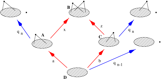
Figure 9: consistency of remaining general covariance conditions

Discrete general covariance states that the probability of forming a causet is independent of the order in which the elements arise, i.e. it is independent of the corresponding path through the poset of finite causets.

Now, general covariance relations always can be taken to come from ‘diamonds’ in the poset of causets, for the following reason. As illustrated in figure 9, any two parents $A$, $C$ of a causet $B$ will have a common parent $D$ (a “grandparent” of $B$) obtained by removing two suitable elements from $B$. (By assumption $B$ must contain an element whose removal yields $A$ and another element whose removal yields $C$. Then remove these two elements. For example, consider the case where     is the grandchild and it has the parent     (by removing the maximal element of the wedge) and the parent    (by removing the disconnected element). To find the grandparent     remove both maximal elements from     .)

Now, still referring to figure 9, let $|D|=n$ and suppose inductively that all the general covariance relations are satisfied up through stage $n$. A new condition arising at stage $n+1$ says that some path arriving at $B$ via $x$ has the same probability as some other path arriving via $z$. But, by our inductive assumption, each of these paths can be modified to go through $D$ without affecting its probability. Thus, the equality of our two path probabilities reduces simply to $ax=bz$.

Now by Bell causality and lemma 2,

$$\frac{x}{q_{n}}=\frac{b}{q_{n-1}}\,,$$

whence

$$ax=ab\frac{q_{n}}{q_{n-1}}\,.$$

But by symmetry, we also have

$$bz=ba\frac{q_{n}}{q_{n-1}}\,;$$

therefore $ax=bz$, as required. $\Box$

References

- [1] Rafael D. Sorkin. Quantum mechanics as quantum measure theory. Modern Physics Letters A, 9(33):3119–3127, 1994. e-print archive: gr-qc/9401003.
- [2] J.L. Friedman and A. Higuchi. State vectors in higher-dimensional gravity with quantum numbers of quarks and leptons. Nuclear Physics B, 339:491–515, 1990.
- [3] Rafael D. Sorkin. Forks in the road, on the way to quantum gravity. Int. J. Th. Phys., 36:2759–2781, 1997. talk given at the conference entitled “Directions in General Relativity”, held at College Park, Maryland, May, 1993. e-print archive: gr-qc/9706002.
- [4] Rafael D. Sorkin. Spacetime and causal sets. In J. C. D’Olivo, E. Nahmad-Achar, M. Rosenbaum, M.P. Ryan, L.F. Urrutia, and F. Zertuche, editors, Relativity and Gravitation: Classical and Quantum, pages 150–173, Singapore, December 1991. World Scientific. (Proceedings of the SILARG VII Conference, held Cocoyoc, Mexico, December, 1990).
- [5] Luca Bombelli, Joohan Lee, David Meyer, and Rafael D. Sorkin. Space-time as a causal set. Physical Review Letters, 59:521–524, 1987.
- [6] David Reid. Introduction to causal sets: an alternative view of spacetime structure. preprint, 1999.
- [7] Luca Bombelli. Spacetime as a Causal Set. PhD thesis, Syracuse University, December 1987.
- [8] F. Markopoulou and L. Smolin, “Causal evolution of spin networks”, Nuc. Phys. B508: 409-430 (1997) e-print archive: gr-qc/9702025
- [9] J. Ambjørn and R. Loll, “Non-perturbative Lorentzian quantum gravity, causality and topology change”, Nuc. Phys. B 536: 407-434 (1999) e-print archive: hep-th/9805108
- [10] J. Ambjørn, K.N. Anagnostopoulos and R. Loll, “A New Perspective on Matter Coupling in 2d Quantum Gravity”, e-print archive: hep-th/9904012
- [11] Graham Brightwell. Models of random partial orders. In Keele, editor, Surveys in combinatorics, volume 187 of London Math. Soc. Lecture Note Ser., pages 53–83. Cambridge University Press, Cambridge, 1993.
- [12] David P. Rideout and Rafael D. Sorkin. Continuum limit of percolated causal sets. (in preparation).
- [13] David P. Rideout and Rafael D. Sorkin. Scaling behavior of percolated causal sets. (in preparation).
- [14] Béla Bollobás and Graham Brightwell. The structure of random graph orders. Siam J. Discrete Math, 10(2):318–335, May 1997.
- [15] Alan Daughton, Rafael D. Sorkin, and C.R. Stephens. Percolation and causal sets: A toy model of quantum gravity. (in preparation).
- [16] David A. Meyer. The Dimension of Causal Sets. PhD thesis, Massachusetts Institute of Technology, 1988.
- [17] Béla Bollobás and Graham Brightwell. Graphs whose every transitive orientation contains almost every relation. Israel Journal of Mathematics, 59(1):112–128, 1987.
- [18] C. M. Newman and L. S. Schulman. One-dimensional percolation models: the existence of a transition for . Comm. Math. Phys., 104(4):547–571, 1986.
- [19] David P. Rideout. Causal Set Dynamics. PhD thesis, Syracuse University, 1999. (in preparation).
- [20] William Feller. An Introduction to Probability Theory and Its Applications, volume I. Wiley, 1957.
- [21] Claude Itzykson and Jean-Michel Drouffe. Statistical Field Theory, volume 2. Cambridge University Press, 1989.
- [22] V. N. Plechko. Anticommuting integrals and fermionic field theories for two-dimensional Ising models. August 1997. e-print archive: hep-th/9607053.
- [23] V.A. Kazakov, “The appearance of matter fields from quantum fluctuations of 2D-gravity”, Mod. Phys. Lett. A 4:: 2125-2139 (1989)
- [24] Matthias Staudacher, “The Yang-Lee edge singularity on a dynamical planar random surface”, Nuc. Phys. B336: 349-362 (1990)
- [25] Alan Daughton. The Recovery of Locality for Causal Sets and Related Topics. PhD thesis, Syracuse University, 1993.
- [26] Roberto Salgado. PhD thesis, Syracuse University, 1999. (in preparation).
- [27] A. Criscuolo and H. Waelbroeck. Causal set dynamics: A toy model. 1998. e-print archive: gr-qc/9811088.