gr-qc/9904045
ISE RR 99/110

Einstein equations in the null quasi-spherical gauge III:
numerical algorithms

Robert Bartnik and Andrew H. Norton
School of Mathematics and Statistics
University of Canberra
ACT 2601, Australia

We describe numerical techniques used in our construction of a 4th order in time evolution for the full Einstein equations, and assess the accuracy of some representative solutions. The scheme employs several novel geometric and numerical techniques, including a geometrically invariant coordinate gauge, which leads to a characteristic-transport formulation of the underlying hyperbolic system, combined with a “method of lines” evolution; a convolution spline for radial interpolation, regridding, differentiation and noise suppression; representations using spin-weighted spherical harmonics; and a spectral preconditioner for solving a class of 1st order elliptic systems on $S^{2}$. Initial data for the evolution is unconstrained, subject only to a mild size condition. For sample initial data of “intermediate” strength ($19\%$ of the total mass in gravitational energy), the code is accurate to 1 part in $10^{5}$, until null time $z=55\textsc{M}$ when the coordinate condition breaks down.

This project has been supported by Australian Research Council grants A69330046 and A69802586.

1 Introduction

The Einstein equations present difficulties of size and complexity somewhat greater than those normally encountered in scientific computation. A numerical simulation must confront a range of theoretical and numerical challenges, starting with the theoretical problem of finding a well-posed and geometrically natural reduction of the full system of Einstein equations. Numerical algorithms are then needed to control the various facets of the reduced system, efficiently, since very large data structures are inevitable when modelling fully 3+1-dimensional spacetimes. Finally there are the twin theoretical and practical problems of understanding the nature of the solution represented by the data, and of certifying its reliability.

In [5] we presented a new coordinate formulation for the vacuum Einstein equations, based on a characteristic (null) coordinate and a quasi-spherical foliation [4]. This null quasi-spherical (NQS) formulation is well-adapted to modelling spacetimes containing a single black hole, extending from the black hole to null infinity.

The purpose of this paper is to describe the numerical algorithms we have used in our implementation of the NQS Einstein equations, and to present results of some accuracy tests of the code. Interactive access to the data sets described here, and many other simulations, is available online at http://gular.canberra.edu.au/relativity.html. More detailed discussions of the physical and geometric significance of the results of the code will be presented elsewhere.

From the numerical programming viewpoint, the most significant features of the code are:

1. a characteristic coordinate $z\sim t-r$ (cf. [56]) plays the role of “time”, with the numerical evolution in the direction of increasing $z$;

2. the numerical grid is based on spherical polar coordinates on the $z$-level sets $\mathcal{N}_{z}$;

3. $S^{2}$ dependencies are handled by a combination of spectral coefficients with respect to a basis of spin-weighted spherical harmonics (for spins $0,1,2$, corresponding to scalar, vector and tensor harmonics); values of the field on a uniform grid in the spherical polar coordinates $(\vartheta,\varphi)$; and Fourier coefficients of the values on the polar coordinate grid;

4. a non-uniform radial grid along the outgoing null hypersurfaces $\mathcal{N}_{z},$ which compactifies future null infinity $\mathcal{I}^{+}$ and is adjusted dynamically so radial grid points approximately follow the inward null geodesics;

5. reformulations of the hypersurface (radial) Einstein equations which enable the numerical modelling of the asymptotic expansions of fields near null infinity;

6. 4th order Runge-Kutta time evolution;

7. the characteristic transport (hypersurface, radial) equations are treated as a system of ordinary differential equations and integrated using an 8th order Runge-Kutta method [46];

8. an 8th order convolution spline is used for interpolation, for computing radial derivatives, to realign the fields with the dynamically varying radial grid, and for suppressing high frequency modes;

9. a first order elliptic system on $S^{2}$ is solved at each radius and time step by the conjugate gradient method, accelerated by a geometrically natural spectral preconditioner.

A number of numerical consistency checks suggest that most quantities of interest which are calculated by the code (eg., the NSQ metric functions, the connection coefficients and the Weyl curvature spinors) have relative errors of about $0.001\%$, for simulations where the gravitational waves carry no more than 20% of of the total spacetime mass. Of course, greater accuracy is found for more nearly linear, weak field, simulations. The major limiting factor in determining the accuracy appears to be the spherical harmonic resolution, currently at $L\leq 15$. Although we have implemented routines which extend this to $L\leq 31$, a full implementation is not possible due to limitations in our present hardware.

The algorithm was initially developed and tested on a 300MHz DEC Alpha with 512Mb memory, and presently runs on a 300MHz Sun Ultra 2 with 784Mb, with a typical (L=15) run taking between 2 and 4 days. Preliminary descriptions of these results are given in [6, 10, 8, 39, 40].

The Cauchy and characteristic initial value problems differ significantly in the nature of their appropriate initial conditions. The Cauchy problem initial data consists of the initial 3-metric and extrinsic curvature [54], whereas the appropriate initial data for a characteristic initial surface is just the null metric. In the NQS case the null metric is

$$ds^{2}_{\mathcal{N}_{z}}=(r\,d\vartheta+\beta^{1}\,dr)^{2}+(r\sin\vartheta\,d\varphi+\beta^{2}\,dr)^{2},$$ (1)

parameterised by the angular shear vector $\beta={\textstyle{\frac{1}{\sqrt{2}}}}(\beta^{1}-{\rm i}\,\beta^{2})=\beta(z,r,\vartheta\,\varphi)$. Unlike the Cauchy problem, the NQS Einstein equations [5] do not impose any additional algebraic or differential constraints on $\beta$, so the initial data $\beta(z=0)$ is an arbitrary function of the spherical polar coordinates $(r,\vartheta\,\varphi)$, except for a mild size constraint (19). Heuristically $\beta$ represents the in-going gravitational radiation of the spacetime; an interpretation which is consistent with the initial ($z=0$) values of $\beta$ being freely specifiable. Note that the geometric invariant $\sigma_{NP}/\rho_{NP}$ [43] becomes $-2\eth\beta/(2-{\mbox{div}}\beta)$ in the NQS coordinates [5].

The NQS geometric gauge provides a formulation of the Einstein equations as an explicit characteristic transport system, coupled to a time evolution equation. This type of structure is also found in characteristic formulations of other hyperbolic equations such as the wave equation, and it is well-known for the Einstein equations in other characteristic coordinate based gauges [28, 50, 56, 37]. Although there are existence results for characteristic initial value formulations of hyperbolic equations, these rely on reduction to the Cauchy problem [48, 66] rather than directly on the transport form. The only exception of which we are aware is the analysis of the linear wave equation in [2, 3]. It would be valuable to have theoretical existence results for systems of characteristic transport equations, which could justify the numerical formulation described here.

The characteristic-based approach has recently been strongly advocated by Winicour and his coworkers [12, 26, 25], who have developed codes for solving the scalar wave equation [26], axially symmetric spacetimes [24] and for the full Einstein equations [11], based on the Bondi coordinate system [28]. These works have been fundamental in establishing the feasibility of numerical formulations based on a characteristic coordinate and in motivating the present implementation. However, the stability analyses and experience of [26, 24] are not directly applicable to our evolution procedure, since the formulations and numerical methods used have several significant differences. Like the Bondi parameterisation, the gauge conditions are directly implemented in the metric form; however, the NQS Einstein equations are considerably simpler than the Bondi coordinate form of the equations [5, 11].

The treatment of angular derivatives is greatly simplified by the quasi-spherical condition, which encourages the use of spherical harmonic expansions. These in turn will simplify comparisons with theoretical results on perturbations of the Schwarzschild black hole [47, 65, 35, 19]. We note that the power of spectral methods in practical applications is well-known, in fields such as meteorology [17], astrophysics [13], and fluid dynamics [18]. Finally, the combination of the characteristic-transport and method of lines techniques, considerably simplifies the use of high order algorithms such as RK4 for time evolution.

The method of lines approach to evolution equations is common in fluid dynamics [18], but has not previously been attempted in numerical relativity. The situation we consider here, of smooth variations in a single black hole geometry, is well-suited to the method, since high frequency modes are less likely to be of physical interest and thus may be treated by smoothing or artificial viscosity.

The use of higher order methods, together with spherical harmonics and radial smoothing, leads to considerably more accurate results than would be possible with the 2nd order methods more commonly employed. However, this suggests that our code is restricted to very smooth spacetimes, and cannot reliably treat spacetimes with strong localised features (such as planets, or gravitational shocks). Because we are concerned primarily with the gravitational wave perturbation modes of a single black hole, this does not present an important restriction, since the dominant modes are known to occur only for low angular momentum $l$ – in particular, the $l=2,3,4$ modes are expected to carry practically all the radiated gravitational energy.

The code models evolution in an exterior domain, and consequently boundary data must also be prescribed at an interior boundary surface $r=r_{0}$. In general only two pieces of the boundary data can be freely specified, thereby fixing the null hypersurfaces $\mathcal{N}_{z}$ and the outgoing radiation flux at the boundary [5]. The rest of the boundary data is constrained by boundary evolution equations (see (26),(27)). For simplicity, the version of the code reported here assumes fixed boundary conditions, corresponding to the past horizon of a Schwarzschild black hole. This assumption considerably simplifies the treatment of the inner boundary, and is completely consistent with the Einstein evolution. It follows that the code models the interaction of gravitational waves with a single Schwarzschild-like black hole. Future versions of the code will incorporate dynamical inner boundary conditions.

The paper is organised as follows.

Section 2 gives the NQS form of the equations, and describes the structure of the equations and the formal steps in the solution algorithm. The geometric significance of the resulting equations is described in [5].

Section 3 describes the numerical techniques used, including the representation of spin-weighted spherical harmonics used to encode the angular variation of the various fields, and the high order convolution splines used for interpolation and differentiation in the radial direction.

Two aspects of the treatment of spherical fields appear to be non-standard [42, 17]: the use of FFT’s in both the $\varphi$ and $\vartheta$ directions, based on the “torus” model of $S^{2}$ [39]; and the use of spin-weighted spherical harmonics to handle, in a unified and frame-invariant manner, vector and higher rank tensor harmonics as well as invariant derivative operators.

Section 4 describes the various stages in the evolution algorithm — solving the hypersurface equations out to null infinity $\mathcal{I}^{+}$; reconstructing the metric from the connection variables (which includes the solution of a 1st order elliptic system on the 2-sphere at each radial grid position); and the evolution of the primary field $\beta$.

In section 5 we describe various techniques for estimating the accuracy of the code, testing both numerical and geometric properties of the numerical solution. Numerical convergence tests estimate the effects of separately increasing the resolution in the radial, time and angular directions. The two geometric tests described here demonstrate the consistency of the numerical metric by verifying the constraint equations for the Einstein tensor components $G_{nn},G_{nm}$ (26,27), and by testing the accuracy of the solution at infinity using the Trautman-Bondi mass decay formula [63, 64, 14, 28]. These provide highly nontrivial tests of the consistency of the numerical solution.

Other tests of the code, based on geometric properties of vacuum spacetimes, and comparisons with known exact and approximate solutions of the Einstein equations, are envisaged for future work.

2 Einstein equations and NQS metric functions

2.1 Spacetime metric

We consider spacetimes admitting global null-polar coordinates $(z,r,\vartheta,\varphi)$ in which the metric takes the null quasi-spherical form [5]

$$ds^{2}_{NQS}=-2u\,dz(dr+v\,dz)+(r\,d\vartheta+\beta^{1}\,dr+\gamma^{1}\,dz)^{2}+(r\sin\vartheta\,d\varphi+\beta^{2}\,dr+\gamma^{2}\,dz)^{2},$$ (2)

where $u>0,v$, and $\beta=\beta^{1}\partial_{\vartheta}+\beta^{2}\csc\vartheta\partial_{\varphi}$, $\gamma=\gamma^{1}\partial_{\vartheta}+\gamma^{2}\csc\vartheta\partial_{\varphi}$ are the unknown NQS metric functions, to be determined by numerical solution of the Einstein equations. Note that we use $\partial_{\vartheta},\partial_{\varphi}$ to denote equivalently the coordinate tangent vectors and the coordinate partial differential operators $\frac{\partial}{\partial\vartheta}$, $\frac{\partial}{\partial\varphi}$. We may consider $\beta,\gamma$ either as vector fields on $S^{2}$ or as spin 1 quantities, defined by the complex combinations [23]

$$\beta={\textstyle{\frac{1}{\sqrt{2}}}}(\beta^{1}-{\rm i}\,\beta^{2}),\qquad\gamma={\textstyle{\frac{1}{\sqrt{2}}}}(\gamma^{1}-{\rm i}\,\gamma^{2}).$$ (3)

The canonical example of a spacetime with metric in NQS form is Schwarzschild spacetime in Eddington-Finkelstein retarded coordinates [20, 30]

$$ds^{2}_{Schw}=-2dz\,(dr+{\textstyle{\frac{1}{2}}}(1-2\textsc{M}/r)\,dz)+r^{2}(d\vartheta^{2}+\sin^{2}\vartheta\,d\varphi^{2})$$ (4)

with $u=1$, $v={\textstyle{\frac{1}{2}}}(1-2\textsc{M}/r)$, $\beta^{A}=\gamma^{A}=0$ and $\textsc{M}=const$. This includes Minkowski space $\mathbb{R}^{3,1}$ as the case $\textsc{M}=0$ and $z=t-|x|$.

2.2 Edth

Using the complex notation (3), we have the canonical angular covariant derivative operator “edth” [23, 44, 21],

$$\eth\eta=\frac{1}{\sqrt{2}}\sin^{s}\vartheta\left(\frac{\partial}{\partial\vartheta}-\frac{{\rm i}\,}{\sin\vartheta}\frac{\partial}{\partial\varphi}\right)\left(\eta\,\sin^{-s}\vartheta\right)=\frac{1}{\sqrt{2}}\left(\frac{\partial}{\partial\vartheta}-s\cot\vartheta-\frac{{\rm i}\,}{\sin\vartheta}\frac{\partial}{\partial\varphi}\right)\,\eta,$$ (5)

acting on a spin $s$ field $\eta$, and its “conjugate” operator $\bar{\eth}$,

$$\bar{\eth}\eta=\frac{1}{\sqrt{2}}\left(\frac{\partial}{\partial\vartheta}+s\cot\vartheta+\frac{{\rm i}\,}{\sin\vartheta}\frac{\partial}{\partial\varphi}\right)\,\eta.$$ (6)

All geometric angular derivative operators may be defined in terms of $\eth$, $\bar{\eth}$. For example, the covariant directional derivative of a spin $s$ field $\eta$ in the direction $\beta$ is

$$\nabla_{\beta}\eta=\beta\bar{\eth}\eta+\bar{\beta}\eth\eta\ ;$$

the divergence and curl (of a vector) are

$${\mbox{div}}\beta = \bar{\eth}\beta+\eth\bar{\beta}=\nabla_{1}\beta^{1}+\nabla_{2}\beta^{2},$$ (7)

$${\mbox{curl}}\beta = {\rm i}\,(\bar{\eth}\beta-\eth\bar{\beta})=\nabla_{2}\beta^{1}-\nabla_{1}\beta^{2}\ ;$$ (8)

and the spherical Laplacian is

$$\Delta\eta=(\eth\bar{\eth}+\bar{\eth}\eth)\eta\ .$$ (9)

Further properties of edth are described in section 3 and in [21, 44, 5].

2.3 Connection variables

In addition to the metric functions $(u,v,\beta,\gamma)$ we introduce the connection fields $H,J,K,Q,Q^{\pm}$

$$H = \frac{1}{u}(2-{\mbox{div}}\beta),$$ (10)

$$J = v(2-{\mbox{div}}\beta)+{\mbox{div}}\gamma,$$ (11)

$$K = v\eth\beta-\eth\gamma,$$ (12)

$$Q = r\frac{\partial\beta}{\partial z}-r\frac{\partial\gamma}{\partial r}+\gamma+\nabla_{\beta}\gamma-\nabla_{\gamma}\beta,$$ (13)

$$Q^{\pm} = \frac{1}{u}(Q\pm\eth u).$$ (14)

Observe that $u,v,H,J$ are real and have spin 0, whereas $\beta,\gamma,Q,Q^{+},Q^{-}$ have spin 1 and $K$ has spin 2.

Given the metric functions $u,v,\beta,\gamma$ on a $z$-level set $\mathcal{N}_{z}$, we may construct $H,J,K$ on $\mathcal{N}_{z}$ directly, and $Q$ (and $Q^{\pm}$) may be reconstructed if in addition, $\partial\beta/\partial z$ is also known on $\mathcal{N}_{z}$. It is clear from (10–14) that this construction does not require any compatibility conditions on the data $u,v,\beta,\gamma,\frac{\partial}{\partial z}\beta$.

Rather remarkably, there is a converse construction for the metric functions $u,v,\gamma$ and $\partial\beta/\partial z$, which also involves totally free and unconstrained data, namely the connection variables $H,J,K,Q$. This contrasts sharply with the description of the connection via the Newman-Penrose spin coefficients [36, 44], which requires numerous differential constraint equations, expressing the property that the connection is torsion-free.

The converse construction works as follows. Given $\beta$ and the connection variables ($H,J,K$) on $\mathcal{N}_{z}$, we reconstruct $u$ via the relation

$$u=\frac{2-{\mbox{div}}\beta}{H},$$ (15)

and we find $v,\gamma$ by solving an elliptic system for $\gamma$,

$$\mathcal{L}_{\beta}\gamma:=\eth\gamma+\frac{\eth\beta}{2-{\mbox{div}}\beta}\,{\mbox{div}}\gamma=J\frac{\eth\beta}{2-{\mbox{div}}\beta}-K,$$ (16)

and setting

$$v=\frac{J-{\mbox{div}}\gamma}{2-{\mbox{div}}\beta}.$$ (17)

The system (16) is $\mathbb{R}$-linear and elliptic with 6-dimensional kernel, provided $\eth\beta$ is not too large ($|\eth\beta|<(2-{\mbox{div}}\beta)/\sqrt{3}$ is sufficient). Prescribing the $l=1$ spherical harmonic coefficients of $\gamma$ (for example, by requiring $\gamma_{l=1}=0$) suffices to determine the solution $\gamma$ uniquely. The remaining connection parameter $Q$, together with the now known values of $\beta,\gamma$ on $\mathcal{N}_{z}$, determines the evolution equation

$$\frac{\partial\beta}{\partial z}=\frac{\partial\gamma}{\partial r}+\frac{1}{r}(Q+\nabla_{\gamma}\beta-\nabla_{\beta}\gamma-\gamma).$$ (18)

To summarise, given the field $\beta$ on a single level set $\mathcal{N}_{z}$, satisfying the size constraint

$$|\eth\beta|<(2-{\mbox{div}}\beta)/\sqrt{3},$$ (19)

the map $(u,v,\gamma,\beta_{z})\mapsto(H,J,K,Q,\gamma_{l=1})$ is invertible, assuming all fields are sufficiently smooth. In section 4.4 we will describe the numerical implementation of the inverse map.

2.4 NQS Einstein equations

To compute the curvature of $ds^{2}_{NQS}$, and thereby to determine the NQS form of the Einstein equations, we introduce the complex null vector frame $(\ell,n,m,\bar{m})$,

$$\ell = \partial_{r}-r^{-1}\beta,$$

$$n = u^{-1}(\partial_{z}-r^{-1}\gamma-v(\partial_{r}-r^{-1}\beta)),$$ (20)

$$m = \frac{1}{r\sqrt{2}}(\partial_{\vartheta}-{\rm i}\,\csc\vartheta\,\partial_{\varphi}),$$

and the directional derivative operators

$$\mathcal{D}_{r}=\partial_{r}-r^{-1}\nabla_{\beta}\,,\quad\quad\mathcal{D}_{z}=\partial_{z}-r^{-1}\nabla_{\gamma}.$$ (21)

Expressions for the Newman-Penrose spin coefficients [36] with respect to the frame $(\ell,n,m,\bar{m})$ are given in terms of $H,J,K,Q$ in [5].

The frame components of the Einstein tensor $G_{ab}$, $a,b=\ell,n,m,\bar{m}$, may be written in terms of the NQS metric functions and NQS connection variables. These expressions may be grouped into hypersurface equations (or main equations [28, 51]):

$$r\mathcal{D}_{r}H = \left({\textstyle{\frac{1}{2}}}{\mbox{div}}\beta-\frac{2|\eth\beta|^{2}+r^{2}G_{\ell\ell}}{2-{\mbox{div}}\beta}\right)H,$$ (22)

$$r\mathcal{D}_{r}Q^{-} = (\eth\bar{\beta}-uH)Q^{-}+\bar{Q}^{-}\eth\beta+2\bar{\eth}\eth\beta{}+u\eth H-H\eth u+2r^{2}G_{\ell m},$$ (23)

$$r\mathcal{D}_{r}J = -(1-{\mbox{div}}\beta)J+u-{\textstyle{\frac{1}{2}}}u|Q^{+}|^{2}{}-{\textstyle{\frac{1}{2}}}u\,{\mbox{div}}(Q^{+})-ur^{2}G_{\ell n},$$ (24)

$$r\mathcal{D}_{r}K = \left({\textstyle{\frac{1}{2}}}{\mbox{div}}\beta+{\rm i}\,{\mbox{curl}}\beta\right)K-{\textstyle{\frac{1}{2}}}J\eth\beta{}+{\textstyle{\frac{1}{2}}}u\eth Q^{+}+{\textstyle{\frac{1}{4}}}u(Q^{+})^{2}+{\textstyle{\frac{1}{2}}}ur^{2}G_{mm},$$ (25)

the boundary equations (or subsidiary equations)

$$r\,\mathcal{D}_{z}\left({J/u}\right) = {v^{2}}\,r\mathcal{D}_{r}\left(J/(uv)\right)+{\textstyle{\frac{1}{2}}}({\mbox{div}}\gamma-v\,{\mbox{div}}\beta)J/u+2u^{-1}|K|^{2}$$ (26)

$${}-\nabla_{Q^{+}}v-\Delta v+u{r^{2}}G_{nn},$$

$$r\,\mathcal{D}_{z}Q^{+} = (v\,r\mathcal{D}_{r}+J-v\eth\bar{\beta}+\eth\bar{\gamma})Q^{+}-K\bar{Q}^{+}+2\bar{\eth}K+2u^{-1}r\mathcal{D}_{r}(u\eth v)$$ (27)

$${}-(2+{\rm i}\,{\mbox{curl}}\beta)\eth v+\eth J-2u^{-1}J\eth u-2ur^{2}G_{nm},$$

and the trivial equation

$$ur^{2}G_{m\bar{m}} = r\mathcal{D}_{r}J-{\textstyle{\frac{1}{2}}}{\mbox{div}}\beta\,J-u|Q^{+}|^{2}+{\textstyle{\frac{1}{2}}}u\,{\mbox{div}}Q^{+}+\bar{Q}^{+}\eth u+Q^{+}\bar{\eth}u$$ (28)

$${}+\bar{K}\eth\beta+K\bar{\eth}\bar{\beta}+r^{2}(v\mathcal{D}_{r}-\mathcal{D}_{z})(u^{-1}\mathcal{D}_{r}u)+u^{-1}r^{2}\mathcal{D}_{r}(u\mathcal{D}_{r}v).$$

Observe that the hypersurface equations (22–25) have no explicit $z$-derivatives, and they each contain only one radial ($r$) derivative. The form of the connection variables ($H,J,K,Q$) was determined by exactly these properties. Consequently, the hypersurface equations may be written schematically in terms of $U=(H,Q^{-},J,K)$ in the “characteristic-transport” form

$$r\frac{\partial U}{\partial r}=F(\beta(z,r),U(z,r)),$$ (29)

by treating angular derivatives such as $\eth U$ as determined by the set of values $U(z,r)$ on the full $S^{2}$. This system has the effect of transporting the fields $U$ along the characteristic curves with tangent vector $\ell$ which foliate the null hypersurfaces $\mathcal{N}_{z}$.

Note that alternative reformulations of the hypersurface equations are possible, preserving the general characteristic transport structure. For reasons associated with reliably capturing the asymptotic behaviour of the fields, the present version of the code integrates the following radial equations, for the variables $\log(H/2)$ (instead of $H$), $j={\textstyle{\frac{1}{4}}}r(1-HJ)-\textsc{M}$ (instead of $J$) and $rQ^{+}$ (instead of $Q^{-}$):

$$r\partial_{r}\log(H/2) = \nabla_{\beta}\log(H/2)+{\textstyle{\frac{1}{2}}}{\mbox{div}}\beta-\frac{2|\eth\beta|^{2}+r^{2}G_{\ell\ell}}{2-{\mbox{div}}\beta},$$ (30)

$$r\partial_{r}(rQ^{+}) = \nabla_{\beta}(rQ^{+})-(1-2\eth\bar{\beta})(rQ^{+})+\nabla_{rQ^{+}}\beta+2r\eth(r\mathcal{D}_{r}\log u)$$ (31)

$${}+2r\beta-{\rm i}\,r\eth{\mbox{curl}}\beta+2r^{3}G_{\ell m},$$

$$r\partial_{r}j = \nabla_{\beta}j+(j+\textsc{M}-{\textstyle{\frac{1}{2}}}r)({\mbox{div}}\beta-r\mathcal{D}_{r}\log u)$$ (32)

$${}+{\textstyle{\frac{1}{4}}}r(|Q^{+}|^{2}+{\mbox{div}}Q^{+})+{\textstyle{\frac{1}{2}}}r^{3}G_{\ell n},\$$

$$2r\partial_{r}K = 2\nabla_{\beta}K+\left({\mbox{div}}\beta+2{\rm i}\,{\mbox{curl}}\beta\right)K-J\eth\beta$$ (33)

$${}+u\eth Q^{+}+{\textstyle{\frac{1}{2}}}u(Q^{+})^{2}+ur^{2}G_{mm}.$$

Here $\textsc{M}=1$ is a constant which fixes the bare mass of the background Schwarzschild black hole. Of course, the Einstein tensor components in these formulae are set to zero for the vacuum equations.

It is remarkable that the boundary equations (26,27) and the trivial equation (28) may be regarded as compatibility relations, by virtue of the conservation (contracted Bianchi) identity $G_{ab}^{\ \ ;b}=0$ [51, 5]. This identity is valid for any Einstein tensor $G_{ab}$, regardless of the metric. Substituting the hypersurface equations $G_{\ell\ell}=G_{\ell m}=G_{\ell n}=G_{mm}=0$ into the conservation identity, yields equations $HG_{m\bar{m}}=0$ and a propagation system for $G_{nn},G_{nm}$ which has the unique solution $G_{nn}=G_{nm}=0$ if the boundary equations are satisfied on one hypersurface transverse to the outgoing null surfaces $\mathcal{N}_{z}$. Thus in order to construct a solution of the full vacuum Einstein equations, it suffices to satisfy the hypersurface equations everywhere, and the boundary equations just on the boundary surface $r=r_{0}$ (for example).

3 Numerical techniques

In this section we describe the data representation and manipulation techniques. These consist mainly of techniques for handling angular fields and derivatives, and an unusual convolution spline used for interpolation, differentiation and high frequency filtering in the radial and time directions.

3.1 Fields on $S^{2}$

The evolution algorithm treats the angular derivatives $\frac{\partial}{\partial\vartheta},\frac{\partial}{\partial\varphi}$ as “lower order”, compared to the radial and time derivatives $\frac{\partial}{\partial r},\frac{\partial}{\partial z}$. This attitude in a numerical computation can be justified only if it is possible to easily and accurately compute and manipulate angular derivatives. This is achieved by using spectral representations (both Fourier and spherical harmonic) for fields on the 2-sphere. This approach is widely used in geophysical and meteorology applications [34, 42, 15, 58, 61] and is known to have significant advantages compared to finite difference approaches [17], based on either angular coordinate grids or overlapping stereographic projection charts [55, 53, 27]. Nevertheless, spectral methods have rarely been used in numerical general relativity (however, see [45, 13]) and they have not been used previously for solving the full Einstein equations.

The basic manipulations required of $S^{2}$ fields are:

• computing non-linear algebraic terms such as $1/(2-{\mbox{div}}\beta)$, $u|Q^{+}|^{2}$ etc;

• computing angular derivatives operators such as ${\mbox{div}}\beta,\ \eth Q^{+}$ etc;

• inverting the linear elliptic operator $\mathcal{L}_{\beta}$ (which appears in equation (16)); and

• projecting aliased or noisy field value data onto certain subspaces of spin-weighted spherical harmonics.

To carry out these manipulations, three separate representations are used for fields on $S^{2}$:

• field values $\eta_{jk}=\eta(\vartheta_{j},\varphi_{k})$ at the polar coordinate grid points

  $$(\vartheta_{j},\varphi_{k})=((j-{\textstyle{\frac{1}{2}}})\Delta\vartheta,(k-1)\Delta\varphi),$$ (34)

  where $\Delta\vartheta=2\pi/N$, $\Delta\varphi=2\pi/N$ with $1\leq j\leq N/2,1\leq k\leq N$ and (in our implementations) $N=16,\,32$ or $64$;

• Fourier coefficients $\hat{\eta}_{mn}$ arising from FFT transforms in the $\vartheta$ or $\varphi$ directions, of the field values $\eta_{jk}$;

• spin-weighted spherical harmonic coefficients $\eta^{lm}$, $|m|\leq l$, $l=s,\ldots,L$, $L=N/2-1$ (for spin $s=0,1$ and 2).

The field value representation is used when computing non-linear algebraic terms such as $u|Q^{+}|^{2}$. The Fourier representation is used for computing $\vartheta$ and $\varphi$ angular derivatives, which are needed in the formulas for $\eth$, div, for example. The spherical harmonic representation is used in solving the elliptic system (16), to spectrally limit the field values by projection to spherical harmonic data, and to summarise the computation results (which are stored using spherical harmonic coefficients).

For fields which do not alias on the $(\vartheta,\varphi)$-grid, the three representations are completely equivalent in the sense that conversion between them is essentially exact, depending on the machine precision and on algebraic details of the specific FFT algorithm used. The requirement that a field does not alias is satisfied when it can be represented by a finite expansion in spin-weighted spherical harmonics with angular momentum $l\leq L=N/2-1$. Our implementations use spectral cutoffs $L=15$ (for $N=32$) and $L=31$ (for $N=64$).

Transformation to the spherical harmonic representation involves a projection, because both the field value and Fourier representations have approximately twice as many degrees of freedom. For example, a (real) spin 0 field with $l\leq L=N/2-1$ has $(L+1)^{2}=N^{2}/4$ spherical harmonic coefficients, whereas it has $N^{2}/2$ values on the $(\vartheta,\varphi)$-grid. The space of non-aliasing spherical harmonics is a linear subspace of the space of functions represented by either Fourier coefficients or field values.

For example, when the $(\vartheta,\varphi)$-grid field values of the product of two fields is calculated, the result, which will contain components up to $l\leq 2L$, is aliased onto the grid in such a way that its field values no longer lie in the appropriate spin weighted spherical harmonic subspace. To clean up after such non-linear effects, we project the result back onto the correct subspace, as described in section 3.5.

To minimise the possibility of unstable feedback of quadratic aliasing errors, we may invoke the Orszag 2/3 rule [18, 41] at various points within the code. The effective spectral resolution of the code is then $l_{\rm max}\approx 2L/3$ ($l_{\rm max}=10$ for $N=32$ and $l_{\rm max}=20$ for $N=64$).

3.2 Spherical harmonics

We first summarise the more important properties of $\eth$ (“edth”) and spin weighted spherical harmonics. The edth formalism provides a unified geometric approach to the treatment of angular derivatives on $S^{2}$ and vector and higher-rank tensor harmonics. Detailed descriptions of the properties of spin-weighted fields and spherical harmonics may be found in Penrose and Rindler [44] or [23, 21]. Here we describe only the basic formulae.

We use a real-valued basis $Y_{lm}$, $l=0,1,2,\ldots$, $m=-l,\ldots,l$ for the space of spin 0 spherical harmonic functions, defined by

$$Y_{lm}=\overline{P}_{lm}(\vartheta)F_{m}(\varphi)\,,$$ (35)

where

$$F_{m}(\varphi)=\left\{\begin{array}[]{cr}1&\quad m=0\\ \sqrt{2}\cos m\varphi&m>0\\ \sqrt{2}\sin|m|\varphi&m<0,\end{array}\right.$$ (36)

and the $\overline{P}_{lm}(\vartheta)=\overline{P}_{l|m|}(\vartheta)$ are related to the associated Legendre functions $P_{lm}$ by

$$\overline{P}_{lm}(\vartheta) = (-1)^{m}\sqrt{2l+1}\sqrt{\frac{(l-m)!}{(l+m)!}}P_{lm}(\cos\vartheta)\,,$$ (37)

$$P_{lm}(\cos\vartheta) = \frac{(-1)^{m}}{2^{l}l!}\sin^{m}\vartheta\left[\frac{d^{l+m}}{dx^{l+m}}(x^{2}-1)^{l}\right]_{x=\cos\vartheta}\,.$$ (38)

The spin $s$ spherical harmonics $Y^{s}_{lm}$ are then defined explicitly by

$$Y^{s}_{lm} = \phantom{(-1)^{s}}\left[\frac{2^{s}(l-s)!}{(l+s)!}\right]^{1/2}\eth^{s}Y_{lm}\,,\qquad s>0,$$ (39)

$$Y^{-s}_{lm} = (-1)^{s}\left[\frac{2^{s}(l-s)!}{(l+s)!}\right]^{1/2}\bar{\eth}^{s}Y_{lm}\,,\qquad-s<0,$$ (40)

where necessarily $l\geq|s|$. Note that the differential operator $\eth$ is spin-raising, sending spin $s$ into spin $(s+1)$ fields, and $\bar{\eth}$ is spin-lowering,

$$\eth Y^{s}_{lm} = \left[{\textstyle{\frac{1}{2}}}(l+s+1)(l-s)\right]^{1/2}Y^{s+1}_{lm},$$ (41)

$$\bar{\eth}Y^{s}_{lm} = -\left[{\textstyle{\frac{1}{2}}}(l+s)(l-s+1)\right]^{1/2}Y^{s-1}_{lm},$$ (42)

for all $s\in\mathbb{Z}$, and $Y^{s}_{lm}$ and $Y^{-s}_{lm}$ are related by complex conjugation,

$$Y^{-s}_{lm}=(-1)^{s}\bar{Y}^{s}_{lm}.$$ (43)

Since $\Delta Y_{lm}=-l(l+1)Y_{lm}$, the fundamental commutation relation

$$[\bar{\eth},\eth]\eta=(\bar{\eth}\eth-\eth\bar{\eth})\eta=s\eta,$$ (44)

for any spin $s$ field $\eta$, may be used to show that

$$\Delta Y^{s}_{lm}=(s^{2}-l(l+1))Y^{s}_{lm},$$ (45)

where $\Delta=\eth\bar{\eth}+\bar{\eth}\eth$. With these conventions we have the orthogonality relations

$$\frac{1}{4\pi}\int_{S^{2}}Y^{s}_{lm}\,\bar{Y}^{s}_{l^{\prime}m^{\prime}}\sin\vartheta\,d\vartheta d\varphi=\delta_{ll^{\prime}}\delta_{mm^{\prime}},$$

which show that the $Y^{s}_{lm}$ form a basis (over $\mathbb{C}$) of the Hilbert space of square-integrable spin $s$ fields on $S^{2}$, which is orthonormal in the natural Hermitian inner product

$$\langle\phi,\psi\rangle=\frac{1}{4\pi}\oint_{S^{2}}{\mbox{Re}}(\bar{\phi}\psi).$$ (46)

From (35–38) it is evident that the spin 0 harmonics $Y_{lm}$ are trigonometric polynomials in $\vartheta$ and $\varphi$ [34]. Using expression (5) for $\eth$, we also see that the $Y^{s}_{lm}$ are trigonometric polynomials. The highest wave number Fourier modes which occur in the set of basis functions $\{Y^{s}_{lm}:s\leq l\leq L,\ |m|\leq l\}$ are $\cos(L\vartheta),\ \sin(L\vartheta),\ \cos(L\varphi)$, and $\sin(L\varphi)$. Therefore, on a uniform $(\vartheta,\varphi)$-grid of size $N/2\times N,$ one can represent all of the spin weighted spherical harmonic functions up to $L=N/2-1$.

3.3 Even/Odd decomposition

Because $\eth$ is surjective onto the space of smooth spin $s$ fields for $s\geq 1$ [44], the decomposition of spin 0 fields or functions into real and imaginary parts may be propagated to higher spin. The resulting decomposition into even and odd components plays an important role in the analysis of the linearised Einstein equations about the Schwarzschild spacetime [47]. Because the NQS geometry distinguishes the Schwarzschild metric and is also based on spherical harmonics, it is ideally suited to comparing nonlinear evolution to the comparatively well-understood black hole linearised Einstein equations [19, 22]. It is thus not surprising that the even-odd decomposition proves to be very important in analysing the results of the NQS evolution.

We say that the spin $s$ field $\eta$ is even if $\eta=\eth^{s}f$ for some real-valued function $f$, and $\eta$ is odd if $\eta={\rm i}\,\eth^{s}g$ for some real-valued function $g$. (If $s<0$ then we interpret $\eth^{s}$ as $(-\bar{\eth})^{|s|}$). This matches the usage in [47] — note that for axially symmetric fields the terms polar (for even) and axial (for odd) are sometimes used [19]. The surjectivity of $\eth$ onto spin $s\geq 1$ ensures that every spin $s$ field may be uniquely decomposed into a sum of even and odd parts. For $s=1$ this decomposition corresponds exactly to the classical Hodge-Helmholtz decomposition of a vector field into the sum of a gradient and a dual gradient (or curl) — see Table 1 for a summary of the various nomenclatures.

Even:	polar	irrotational	$\eth f$	$\textrm{grad}f$	$(\nabla_{1}f)\,v_{1}+(\nabla_{2}f)v_{2}$
Odd:	axial	divergence-free	${\rm i}\,\eth g$	${\mbox{curl}}g$	$(\nabla_{2}g)\,v_{1}-(\nabla_{1}g)v_{2}$

Table 1: Equivalent terminologies for vector fields on $S^{2}$

The even/odd decomposition has a natural interpretation in terms of the spectral decomposition

$$\eta=\sum_{l=s}^{\infty}\sum_{m=-l}^{l}\eta^{lm}Y^{s}_{lm}$$ (47)

of a spin $s$ field $\eta$, because we are using a basis of real-valued $Y_{lm}$. Namely, $\eta$ is even if the spectral coefficients $\eta^{lm}$ are real, and odd if the coefficients are pure imaginary. We sometimes use $\textrm{Even}(\eta)$ and $\textrm{Odd}(\eta)$ to represent the respective projections, so $\eta=\textrm{Even}(\eta)+\textrm{Odd}(\eta)$ with

$$\textrm{Even}(\eta) = \sum{\mbox{Re}}(\eta^{lm})Y^{s}_{lm}$$ (48)

$$\textrm{Odd}(\eta) = {\rm i}\,\sum{\mbox{Im}}(\eta^{lm})Y^{s}_{lm}.$$ (49)

Observe that $\eth Y^{s}_{sm}=0$ for $s\geq 0$ and thus $\eth$ acting on spin $s$ fields with $s\geq 0$ has kernel having (complex) dimension $2s+1$. Likewise the formal adjoint $-\bar{\eth}$ acting on spin $s\leq 0$ fields has $(2|s|+1)$-dimensional kernel. In particular, $\eth$ acting on spin 1 fields has kernel consisting of the $\mathbb{C}$-linear space spanned by the three $l=1$ spin 1 spherical harmonics $Y^{1}_{1m}$ — the corresponding real vector fields are the dual gradients of functions linear in $\mathbb{R}^{3}$, which are just the infinitesimal rotations, and the gradients, which are the conformal dilation vector fields.

The correspondence between vector fields on $S^{2}$ and spin 1 fields generalises to spin 2 fields, which correspond to symmetric traceless 2-tensors on $S^{2}$. If $\lambda$ is a symmetric traceless 2-tensor then with respect to the standard polar coordinate derived orthonormal frame

$$e_{1}=\partial_{\vartheta},\quad e_{2}=\csc\vartheta\,\partial_{\varphi},$$ (50)

we have the correspondence

$$\lambda\sim{\textstyle{\frac{1}{2}}}(\lambda^{11}-\lambda^{22}-2{\rm i}\,\lambda^{12})\,.$$ (51)

This correspondence extends to higher integer spins with higher rank symmetric traceless tensors on $S^{2}$. The cases $s=0,1,2$ of most importance in our work correspond to the usual scalar, vector and tensor harmonics.

3.4 Fourier representation

The fast Fourier transform (FFT) is used to transform between Fourier coefficients and field values on the uniform $(\vartheta,\varphi)$-grid. Fourier convergence problems arising from discontinuities in coordinate derivatives and vector and tensor components at the poles, are sidestepped by an observation relating fields on $S^{2}$ to fields on the torus ${\mathbb{T}}^{2}=S^{1}\times S^{1}$ [39]. The torus method enables coordinate and covariant derivatives for all types of field to be computed using Fourier methods, so is particularly well-suited to handling the derivative operator $\eth$ (5). This approach to handling component discontinuities at the poles is simpler than the techniques reviewed in [59] for manipulating vector fields, and readily extends to any rank $s\geq 0$.

For integer $s$ the real and imaginary parts of a spin $s$ field on $S^{2}$ may be identified with the two independent frame components of a completely symmetric trace-free tensor of rank $|s|$ on $S^{2}$ [44]. Since the frame $e_{1},e_{2}$ (50) is not continuous at the poles, the tensor components will not be continuous at the poles, so are not obviously suited to Fourier expansion in the $\vartheta$ direction.

However, along any smooth curve crossing through a pole, both basis vectors $e_{1}$ and $e_{2}$ reverse direction at the pole. Thus, for any smooth tensor field $T=T^{j_{1}\ldots j_{s}}e_{j_{1}}\otimes\cdots\otimes e_{j_{s}}$, by continuity of $T$ the component functions $T^{j_{1}\ldots j_{s}}$ will change by a factor $(-1)^{s}$ across the poles. Consequently, if we extend the domain of definition of $T^{j_{1}\ldots j_{s}}$ to $\vartheta\in[-\pi,\,\pi]$ by

$$T^{j_{1}\ldots j_{s}}(-\vartheta,\varphi)\;=\;(-1)^{s}T^{j_{1}\ldots j_{s}}(\vartheta,\varphi+\pi)\,,\quad\mathrm{for}\ \vartheta\in[0,\pi]$$ (52)

(using the $2\pi$ periodicity in $\varphi$), then the resulting extension is $2\pi$-periodic and continuous in $\vartheta$. This argument extends to higher (covariant) derivatives of $T$, showing that the extension is in fact smooth and periodic in $\vartheta$. Derivatives of $T^{j_{1}\ldots j_{s}}$ with respect to $\vartheta$ can then be calculated just as for $\varphi$ derivatives, provided that the direction of increasing $\vartheta$ is properly taken into account.

In effect, the extension just described defines a (smooth) field $T^{j_{1}\ldots j_{s}}$ on the torus $\mathbb{T}^{2}=S^{1}\times S^{1}$. This may be understood geometrically by noting that the map

$$\Upsilon:{\mathbb{T}}^{2}\to S^{2},\quad(\vartheta,\varphi)\mapsto\left\{\begin{array}[]{ll}(\vartheta,\varphi),&\vartheta\in(0,\pi],\ \phi\in(-\pi,\pi]\\ (-\vartheta,-\varphi),&\vartheta\in(-\pi,0],\ \phi\in(-\pi,\pi]\\ \end{array}\right.$$ (53)

is in fact smooth. This follows by noting that because $\vartheta$ is a radial coordinate near the north pole $\vartheta=0$, the differential structure near the pole is represented by the rectangular coordinates $(\xi,\eta)=(\vartheta\cos\varphi,\vartheta\sin\varphi)$ and the map $(\vartheta,\varphi)\mapsto(\xi,\eta)$ is manifestly $C^{\infty}$ for $\vartheta$ near $0$. Consequently any smooth tensor $T$ on $S^{2}$, when expressed in a cotangent basis, pulls back to a smooth tensor on ${\mathbb{T}}^{2}$ (ie. $\Upsilon^{*}(T)\in C^{\infty}({\mathbb{T}}^{2})$), and thus admits a well-behaved Fourier representation on ${\mathbb{T}}^{2}$. The converse is of course false: a smooth tensor on ${\mathbb{T}}^{2}$ does not necessarily arise from a smooth tensor on $S^{2}$, even if it satisfies the parity condition (52) satisfied by pull-back tensors.

The coordinate derivative form (5) of $\eth$ (and similarly any other covariant angular derivative operator) can be easily evaluated by transforming to the Fourier representation of the field, multiplying the Fourier coefficients by the appropriate wavenumber factors, transforming back to obtain the field value representation of the $\vartheta$ and $\varphi$ derivatives, then finally including the $\csc\vartheta$ factors. Thus, computing a derivative operator such as $\eth$ is an $O(N^{2}\log N)$ operation. Since $\csc({\textstyle{\frac{1}{2}}}\Delta\vartheta)\simeq 10$ for $N=32$, there is no significant loss of accuracy in calculations near the poles.

It should be emphasised that because the $Y^{s}_{lm}$ are trigonometric polynomials in $(\vartheta,\varphi)$, the FFT computation of their numerical derivatives is algebraically exact. For example, the Laplacian relation (45) is numerically verified to 1 part in $10^{12}$ [39].

3.5 The spherical harmonic representation

The field value and Fourier representations suffice for most numerical calculations, such as computing the nonlinear terms in (22–25). However, at some steps it is essential to use the representation by spherical harmonic coefficients (47):

1. to solve the elliptic system (16) (see section 4.4);

2. to implement spectral projections after each time step, with the aim of suppressing aliasing effects and rounding errors at the poles [42];

3. to store results for later analysis and display, since the spherical harmonic representation is more compact and the coefficients may be readily interpreted physically, by comparison with well-studied solutions of the linearised black hole Einstein equations [47, 65, 19].

We next describe the methods used to transform fields from the field value and Fourier representations to the spherical harmonic representation. Transformations for fields of spin 0, 1 and 2 are required by the code; the spin 0 case which we describe here to illustrate the technique is slightly less complicated, since we may assume the field $f$ is real-valued.

There are $(L+1)^{2}$ basis functions in the set $\{Y_{lm}:0\leq|m|\leq l\leq L\}$. However, to represent these functions as trigonometric polynomials on a regular $S^{2}$ grid we require a grid of size $(L+1)\times 2(L+1)$, and thus $2(L+1)^{2}$ real coefficients. The spin 0 functions of angular momentum at most $L$ therefore form a subspace of real dimension $(L+1)^{2}$ in the space of Fourier series representable on the grid, which has real dimension $2(L+1)^{2}$. We use a projection onto the spherical harmonic subspace which is orthogonal with respect to the natural inner product in the Fourier space,

$$\langle f_{1},\,f_{2}\rangle_{2} = \frac{1}{4\pi^{2}}\int_{0}^{2\pi}\int_{0}^{2\pi}f_{1}(\vartheta,\varphi)f_{2}(\vartheta,\varphi)d\vartheta d\varphi$$ (54)

$$= \frac{1}{N^{2}}\sum_{i=1}^{N}\sum_{j=1}^{N}f_{1}(\vartheta_{i},\varphi_{j})f_{2}(\vartheta_{i},\varphi_{j})\,,$$

where $\{(\vartheta_{i},\varphi_{j}):i,j=1,\ldots,N\}$ are grid points (cf. (34)) and $N=2(L+1)$.

To make use of (54) we use (52) to extend functions defined on $S^{2}$ to functions defined on the torus $\mathbb{T}^{2}=S^{1}\times S^{1}$. In particular, given any set of values $\{f_{ij}\in\mathbb{R}:i=1,\ldots,N/2,\ j=1,\ldots,N\}$ on the $S^{2}$ grid, we use (52) to construct grid values on $\mathbb{T}^{2}.$ There is then a unique interpolating trigonometric polynomial $f$ such that $f(\vartheta_{i},\varphi_{j})=f_{ij}$. We project $f$ to the $l\leq L$ spherical harmonic subspace as follows.

The $Y_{lm}$ are not orthonormal with respect to (54), but instead have Fourier inner product

$$G_{lm\;l^{\prime}m^{\prime}} = \langle Y_{lm},\,Y_{l^{\prime}m^{\prime}}\rangle_{\textsc{F}}$$ (55)

$$= \langle\overline{P}_{lm}(\vartheta),\,\overline{P}_{l^{\prime}m}(\vartheta)\rangle_{\textsc{F}}\,\delta_{mm^{\prime}}\,.$$

Here, the index pair $lm$ (and $l^{\prime}m^{\prime}$) is a combined index which takes $(L+1)^{2}$ values, and (55) is the matrix for the induced Fourier metric on the spin 0 subspace. The summation convention will be employed for raised and lowered repeated indices.

For fixed $m$, the inner product (55) of the $\overline{P}$ functions forms a matrix,

$$A_{(m)ll^{\prime}}=\langle\overline{P}_{lm}(\vartheta),\,\overline{P}_{l^{\prime}m}(\vartheta)\rangle_{\textsc{F}}\,.$$

These matrices are defined only for $|m|\leq l,l^{\prime}\leq L$, so are square and of size $(L+1-|m|)\times(L+1-|m|)$. Denoting the inverse matrix by $A_{(m)}^{ll^{\prime}}$, we have

$$G_{lm\;l^{\prime}m^{\prime}}=A_{(m)ll^{\prime}}\delta_{mm^{\prime}}\,,$$ (56)

and the components of the inverse metric are given by

$$\quad\quad\quad\quad\quad G^{lm\;l^{\prime}m^{\prime}}=A_{(m)}^{ll^{\prime}}\delta^{mm^{\prime}}\ \quad(\mbox{no sum on}\ m).$$ (57)

The dual basis vectors for the spin 0 subspace are

$$Y^{lm}=G^{lm\;l^{\prime}m^{\prime}}Y_{l^{\prime}m^{\prime}}\,,$$ (58)

and satisfy $\langle Y_{lm},\,Y^{l^{\prime}m^{\prime}}\rangle_{\textsc{F}}=\delta^{l^{\prime}}_{l}\delta^{m^{\prime}}_{m}\,$. The orthogonal projection of $f$ onto the subspace is given by

$${\rm proj}(f)=\langle f,\,Y^{lm}\rangle_{\textsc{F}}Y_{lm}=f^{lm}Y_{lm},$$

where

$$f^{lm}=\langle f,\,Y^{lm}\rangle_{\textsc{F}}$$ (59)

are the spherical harmonic coefficients of the function $f$.

To calculate the inner product (59), first note that using (35), (57) and (58), the dual basis vectors can be written as

$$Y^{lm}=\overline{P}^{lm}(\vartheta)F^{m}(\varphi)\,$$ (60)

(in analogy with (35)), where we have set

$$\overline{P}^{lm}(\vartheta)=A_{(m)}^{ll^{\prime}}\overline{P}_{l^{\prime}m}(\vartheta)\,,\quad F^{m}(\varphi)=F_{m}(\varphi).$$ (61)

By Fourier analysis of $f$ in the $\varphi$ direction we can write $f=\hat{f}^{k}(\vartheta)F_{k}(\varphi)$. In particular, by $\varphi$-FFT of $\{f_{ij}\}$ we get the numbers $\hat{f}^{k}(\vartheta_{i})$. The spectral coefficients $f^{lm}$ can then be evaluated using (54) and (60) as

$$f^{lm} = \langle\hat{f}^{k}(\vartheta)F_{k}(\varphi),\,\overline{P}^{lm}(\vartheta)F^{m}(\varphi)\rangle_{\textsc{F}}$$ (62)

$$= \langle\hat{f}^{m}(\vartheta),\,\overline{P}^{lm}(\vartheta)\rangle_{\textsc{F}}$$

$$= \frac{1}{N}\sum_{i=1}^{N}\hat{f}^{m}(\vartheta_{i})\overline{P}^{lm}(\vartheta_{i})\,.$$

The converse process of reconstructing the function values $f_{ij}=f(\vartheta_{i},\varphi_{j})$ from the spherical harmonic coefficients $f^{lm}$ follows from

$$f = f^{lm}\,Y_{lm}(\vartheta,\varphi)$$

$$= f^{lm}\overline{P}_{lm}(\vartheta)F_{m}(\varphi)\,.$$

First we construct the quantities

$$\quad\quad\quad\quad\quad\hat{f}^{m}(\vartheta_{i})=\sum_{l=|m|}^{L}f^{lm}\overline{P}_{lm}(\vartheta_{i})\,,\ \quad(\mbox{no sum on}\ m),$$ (63)

and then we use inverse FFTs in the $\varphi$ direction to reconstruct $f_{ij}$ via

$$f_{ij}=\sum_{m=-L}^{L}\hat{f}^{m}(\vartheta_{i})F_{m}(\varphi_{j})\,.$$

Both constructions, of $f^{lm}$ from $f_{ij}$ and conversely, are $O(L^{3})$ operations, due to the matrix multiplications in (62), (63). Routines for transforming between grid values and spherical harmonic coefficients have been implemented for maximum angular momentum $L=7,15\ {\rm and}\ 31$. The grid values $\overline{P}^{lm}(\vartheta_{i})$ which appear in the sum (62) were pre-computed in multiple precision using REDUCE [31]. The functions $\overline{P}^{lm}(\vartheta)$ defined by (61), were constructed symbolically using exact inversion of the matrices $A_{(m)\,ll^{\prime}}$. This symbolic approach was feasible because the metric $G_{lm\;l^{\prime}m^{\prime}}$ factorized as the tensor product (55), thus allowing exact inversion of $G$ using matrices of size at most $(L+1)\times(L+1)$ rather than $(L+1)^{2}\times(L+1)^{2}$.

The analysis of spin 1 and spin 2 grid functions into spherical harmonic coefficients is similar, but complicated by the fact that the induced metric on the subspace factorizes as a tensor product only in a complex (mixed parity) basis. Separating the even and odd parity coefficients therefore requires some extra book keeping.

Techniques for handling spherical harmonic spectral representations have been described by many authors [34, 42, 58, 17, 32]. Our method differs from the Muchenhauer and Daly projection (see [58]) in the choice of inner product (54) used to define the orthogonal subspace. More general spectral transform methods (eg. [17]) use other choices of weightings and node points to define the projection, and do not have such a simple underlying inner product. All these methods are also $O(L^{3})$. Jakob [32] gives an $O(L^{2}\log L)$ spectral projection, which however bypasses the construction of the spherical harmonic coefficients. Since we need the spectral coefficients, and because we work with a relatively small value of $L$, the Jakob projection would not provide any improvement.

The torus method described here and in [39] has the advantage that it applies also to higher rank tensors, in particular vectors and 2-tensors. Representations in terms of spin-weighted fields are more efficient for vectors (spin $s=1$) than 3-vector representations [59, 60], and the operator $\eth$ gives a transparent derivation of all invariant derivative combinations [59].

3.6 Convolution splines

At various stages it is necessary to interpolate and differentiate grid-based fields. For example, the radial integration of the hypersurface equations by the 8th order Runge-Kutta method requires values of the source field $\beta$ at $10$ intermediate points; the dynamic regridding of the radial grid requires interpolation to determine the field values of $\beta$ at the new grid points; and derivatives such as $\partial\gamma/\partial r$ and $\partial Q^{+}/\partial z$ must be computed from field values on grids. A convolution spline algorithm described in [38] provides a convenient technique.

The method has the effect of fitting a spline curve to sample data, and is implemented by a convolution of the form [38]

$$\bar{f}(x)=\sum_{k\in\mathbb{Z}}f(k)\phi_{n}(x-k),$$ (64)

where the $f(k)$ are the raw data (samples) and $\phi_{n}(x)$ is a $C^{n-2}$ sampling kernel.

The sampling kernel $\phi_{n}$ is constructed as a certain sum of central B-splines $M_{n}$ of order $n,$

$$\phi_{n}(x)=\sum_{i=1}^{n-1}a_{i}^{(n)}M_{n}(x-{\textstyle{\frac{n}{2}}}+i),$$ (65)

where the coefficients $a_{i}^{(n)}$, $i=1,\ldots,n-1$ are chosen so that the convolution (64) acts as the identity on polynomials $f(x)$ of degree $n-1$ ($n$ even) or $n-2$ ($n$ odd). Recall that the central B-spline $M_{n}(x)$ is a $C^{n-2}$ piecewise polynomial of degree $n-1$ normalised by $\sum_{k\in\mathbb{Z}}M_{n}(x-k)=1$, with support on $|x|\leq n/2$ [52]. The support of the kernel $\phi_{n}(x)$ is therefore $|x|\leq n-1.$

Algorithms for computing the $a_{i}^{(n)}$ and tabulations for $n\leq 11$ are given in [38]. Coefficients for the kernel $\phi_{9}$ used in the code are given in Table 2, and $\phi_{9}$ is plotted in Figure 1.

Table 2: Convolution coefficients $a_{i}^{(9)}$.

$i$:	$1,8$	$2,7$	$3,6$	$4,5$
$a_{i}^{(9)}$:	$-\frac{67}{2520}$	$\frac{1111}{5040}$	$-\frac{421}{560}$	$\frac{1333}{1260}$

Figure 1: Comparison of the $C^{7}$ spline kernel $\phi_{9}$ (solid curve) and the sinc method [16, 57] kernel ${\rm sinc}(x)=\sin(\pi x)/\pi x$ (dotted curve). The kernel for a sampling method is the response to the delta-like discrete data (solid dots). The advantages of the convolution spline method are that the kernels have finite support ($[-8,8]$ in this case) and the data is automatically filtered. The convolution (64) using kernel $\phi_{9}$ exactly reproduces polynomials of degree $7$ or less.

The expressions (64), (65) may be rearranged into a form which is more efficient for numerical calculations,

$$\bar{f}(x)=\sum_{k\in\mathbb{Z}}\tilde{f}_{k}M_{n}(x-{\textstyle{\frac{n}{2}}}-k),$$ (66)

where the modified sample values $\tilde{f}_{k}$ are given by

$$\tilde{f}_{k}=\sum_{i=1}^{n-1}f(k+i)a_{i}^{(n)}.$$

The advantage of (66) is that the $\tilde{f}_{k}$ can be computed once and then reused to evaluate $\bar{f}(x)$ at many different points $x$, using the explicitly known values of the B-spline $M_{n}(x).$ The same $\tilde{f}_{k}$ values may also be used to compute derivatives of the spline function $\bar{f}$,

$$\bar{f}^{(j)}(x)=\sum_{k\in\mathbb{Z}}\tilde{f}_{k}M_{n}^{(j)}(x-k-{\textstyle{\frac{n}{2}}}),$$ (67)

where again the derivatives $M_{n}^{(j)}(x)$ are known functions. These techniques are routinely used to supply intermediate values and derivatives of fields in the radial and time directions.

Non-uniform distributions of sample points are handled by a mapping between the independent variable and the sample number variable ($x$ in the above). Numerical derivatives are then calculated using the chain rule. For example, the radial grid described in Section 4.2 is non-uniform, specified by some known relation of the general form $r=r(n)$ (where $n$ is now being used to denote the sample number variable, with radial grid points being at $n=0,\ldots,n_{\infty}$). The operator $\frac{\partial}{\partial r}$ is then implemented as $\left(\frac{dr}{dn}\right)^{-1}\frac{\partial}{\partial n}$, with a formula for the first factor being known explicitly.

Similarly, one can transform to an independent variable $s=s_{0}+hx$ which has grid spacing $h$, to examine the behaviour of the approximation (64) as $h\rightarrow 0.$ Let $g(s):=f((s-s_{0})/h)=f(x)$, so $g^{(j)}(s)=h^{-j}f^{(j)}(x)$. It can be shown [38] that using the $\phi_{9}$ kernel, the Taylor series truncation errors for (64) at a grid point $s$ are

$$|\bar{g}^{(j)}(s)-g^{(j)}(s)|=c_{j}h^{8}|g^{(8+j)}(s)|+O(h^{9}),\quad j=0,1,2,$$ (68)

where $c_{0}=\frac{2021}{134400}$, $c_{1}=\frac{4547}{302400}$, $c_{2}=\frac{4549}{302400}$. This reflects the fact that convolution with $\phi_{9}$ is exact on polynomials of degree $7$.

The predicted $h^{8}$ convergence of the $\phi_{9}$ spline convolution is clearly evident in Figure 2. Here the function $v(x)=e^{x}\sin 10x$ has been approximated at varying grid resolutions corresponding to $N=2^{p}$ grid points over the interval $[-1,1]$.

(a)	(b)

Figure 2: Convergence of the $\phi_{9}$ spline convolution: (a) samples of $v(x)=e^{x}\sin 10x$ at $N=16$ points over $[-1,1]$, and the corresponding convolution spline; (b) logarithmic plots of the absolute error $|v(x)-\bar{v}(x)|$ for grid resolutions of $N=2^{p}$ with $p=4,\ldots,7,$ showing a reduction in the error by a factor of $2^{8}$ on each doubling of the resolution.

Convolution splines do not generally preserve sample values, except for samples from polynomials of degree less than or equal to the degree of reproduction. This results in some damping of high frequency components of the data, which we expect helps to suppress numerical noise and algorithmic instabilities.

Within the context of spectral methods for PDEs, the direct filtering of Fourier coefficients of a numerical solution is common practice and has been extensively studied (cf. [18, §8.3] and references). On the other hand, explicit use of a digital filter [29] in conjunction with finite difference methods is comparatively rare. Nevertheless, from an algorithmic point of view, this is the effect of using a convolution spline.

The filtering inherent in the method can be examined via the response function

$$\Phi_{n}(\theta)=\sum_{k\in\mathbb{Z}}\phi_{n}(k)\cos k\theta,\quad 0\leq\theta\leq\pi,$$ (69)

which is equal to the factor by which the Fourier mode $e^{{\rm i}\,\theta x}$ is amplified by the approximation (64) at a grid point $x\in\mathbb{Z}.$ The value $\theta=\pi$ corresponds to the Nyquist frequency for the grid.

Figure 3 shows the response function $\Phi_{9}(\theta)$, compared to the well-known Lanczos and raised cosine (artificial viscosity) filters [29]. The filtering characteristics of convolution splines and their derivatives are described in [38].

Figure 3: Filter response functions: (a) raised cosine filter $\sigma(\theta)={\textstyle{\frac{1}{2}}}(1+\cos\theta)$; (b) Lanczos filter $\sigma(\theta)=\theta^{-1}\sin\theta$; (c) sharpened raised cosine [18]; (d) $\Phi_{9}(\theta)$.

The limitations of convolution splines are illustrated in Figure 4, which shows Gibbs-like effects associated with approximation of step-like data. The figures also give an indication of the number of grid points needed to resolve a sharp transition in field values.

$\begin{array}[]{cc}\includegraphics{tanh_N16.ps}&\includegraphics{tanh_N64.ps}\\ \includegraphics{tanh_N32.ps}&\includegraphics{tanh_errors.ps}\end{array}$

Figure 4: Convolution spline approximation of step-like data. Here the function $u=\tanh(10x)$ is represented by $N$ samples over the interval $[-3,3]$. For $N=16$, the transition from $u\approx-1$ to $1$ takes just one grid interval and a Gibbs-like phenomenon is evident. The convolution splines are constructed using the $\phi_{9}(x)$ kernel. The logarithmic plot shows the absolute error, $|u(x)-\bar{u}(x)|$.

In order that the convolution spline smoothing should introduce only negligible errors, the grid resolution should be chosen sufficiently fine that typical field variations take place over enough grid points that the expected frequency $\theta$ of the field data lies well within the part of the Nyquist frequency interval where $\Phi_{n}(\theta)\approx 1$. Of course this requires some prior knowledge of the length scale of the field, and cannot be applied where shocks (or arbitrarily rapid variations) occur in the data. In such cases the spherical harmonic representation would become equally unsuitable.

The choice of high order convolution splines ($h^{8}$ rather than say $h^{4}$) was motivated by the need to reduce storage requirements. Low order spline convolutions have a markedly reduced usable proportion of the Nyquist interval [38], so to avoid over-smoothing and to achieve comparable accuracy with a low order method would require significantly higher grid point densities. Both storage costs and the cost of the radial integration increase linearly with the number of radial grid points. The $\phi_{9}$ kernel was chosen also because its accuracy matches that of the RK8 method used for the radial integration.

To use convolution splines near endpoints of a data set, one can extend the data set, using a suitable mapping between the independent variable and the sample number variable [40]. The mapping is chosen so that when expressed in terms of the sample number variable $n$, $0\leq n\leq n_{\infty}$, the fields admit expansions in powers of $n^{2}$ near $n=0$ and $(n_{\infty}-n)^{2}$ near $n=n_{\infty}$. The sampling kernel convolution can then be applied to the even extension of the fields through $n=0$ or $n=n_{\infty}$. This technique is particularly important in extracting radiation data near null infinity (scri, $\mathcal{I}^{+}$), where the radial grid is chosen so that $n_{\infty}-n=O(r^{-1/2})$, as described in Section 4.2.

4 Solution algorithm

The hypersurface equations (22-25) suggest the following process for evolving the metric in the exterior region with interior boundary the cylinder $r=r_{0}$:

1. Choose boundary data $(H,Q^{-},J,K)$ on the cylinder $r=r_{0}$, consistent with the boundary equations (26,27);

2. Assume $\beta$ is given on a null hypersurface $\mathcal{N}_{z}$;

3. Solve the $\mathcal{N}_{z}$ hypersurface equations $r\partial_{r}U=F(\beta,U)$, by integrating along the radial curves $(z,\vartheta,\varphi)=const.$ with initial conditions at $r=r_{0}$ determined in step 1;

4. reconstruct the metric functions $u,v,\gamma$ from $H,J,K$ and $\beta$ using the converse construction (15–17);

5. reconstruct $\partial\beta/\partial z$ from $Q$ and the now known values of $\beta,\gamma$ on $\mathcal{N}_{z}$, using (18);

6. use $\partial\beta/\partial z$ from step 5 to evolve $\beta$ to the “next” null hypersurface $\mathcal{N}_{z+\Delta z}$ and repeat from step 3.

In the following we will show how this heuristic algorithm is implemented numerically, using the techniques and data representations of the previous section.

4.1 Geometry and inner boundary conditions

The code models gravitational waves propagating on a black hole spacetime, with metric approximating that of the Schwarzschild solution in the Kruskal-Szekeres coordinates [30]. Introducing the double-null coordinates

$$z=t-r^{*},\qquad y=t+r^{*},\qquad r^{*}=r+2\textsc{M}\log\left(\frac{r}{2\textsc{M}}-1\right),$$

the Schwarzschild metric becomes

$$ds^{2}_{Schw}=-(1-2\textsc{M}/r)\,dy\,dz+r^{2}d\Omega^{2}\,,$$

where $d\Omega^{2}=d\vartheta^{2}+\sin^{2}\vartheta\,d\varphi^{2}$. The coordinate singularities at the past and future horizons $t=\pm\infty$ are removed by defining $\tilde{y}=e^{y/4\textsc{M}}$, $\tilde{z}=e^{-z/4\textsc{M}}$, giving the metric

$$ds^{2}_{Schw}=\frac{32\textsc{M}^{3}}{r}e^{-r/2\textsc{M}}\,d\tilde{y}d\tilde{z}+r^{2}\,d\Omega^{2}\,,$$

where $r=r(\tilde{y},\tilde{z})$ is defined implicitly by (see Figure 5)

$$e^{r/2\textsc{M}}\left(\frac{r}{2\textsc{M}}-1\right)=\tilde{y}\tilde{z}.$$ (70)

Because radial light rays are straight lines at $45^{\circ}$ and $r=0$ is singular, the surfaces $\tilde{z}=0$ and $\tilde{y}=0$ (ie. $r=2\textsc{M}$) form the past and future event horizons, and these are smooth hypersurfaces with bounded curvature. The approximate Minkowski structure of Schwarzschild spacetime is better illustrated by the radial null geodesics in $(r,t)$ coordinates, see Figure 6. Note however that the $(r,t)$ coordinates are singular along the event horizons $r=2\textsc{M}$.

Figure 5: Schwarzschild spacetime in Kruskal-Szekeres coordinates. Radial light rays are straight lines at $45^{\circ}$.

(a)	(b)

Figure 6: Exterior region $r>2\textsc{M}$ of Schwarzschild spacetime, with past and future radial null geodesics. (a) In Schwarzschild coordinates $(r,t)$; (b) in retarded Eddington-Finkelstein coordinates $(r,z).$

Initial conditions for $\beta$ are imposed on $\{z=0,r\geq 2\textsc{M}\}$ (with $\textsc{M}=1$ usually), by specifying the spherical harmonic coefficient functions $\beta_{lm}(r)$. Since $\beta(z=0)$ is unconstrained, these coefficient functions may be freely chosen, subject only to the size condition (19).

For simplicity the inner boundary conditions are set at $r_{0}=2\textsc{M}=2$ to agree with the Schwarzschild past horizon: $H_{0}=2$, $Q_{0}=J_{0}=K_{0}=0$. Since we choose $\beta(0,r)=0$ for $2\leq r\leq 5$, by causality the solution should agree with the Schwarzschild metric in a neighbourhood of $r=2$ for all time $z\geq 0$, producing a “white hole” past horizon in the spacetime. This choice of inner boundary condition has the considerable advantage that the boundary equations (26),(27) are automatically satisfied, and it is not necessary for this class of simulations to separately ensure that the boundary data are numerically compatible with the boundary equations.

The resulting spacetimes have the geometry of an isolated black hole with future event horizon at $z=\infty$, $r>2\textsc{M}$ and Schwarzschild-like white hole boundary along $r=2\textsc{M},0\leq z<\infty$. Adding shear $\beta$ at the initial hypersurface $z=0$ results in spacetimes modelling the interaction of gravitational radiation with a single black hole.

Although the fixed past horizon boundary conditions used in the present code allow many interesting issues to be addressed, it would be desirable to implement more general inner boundary conditions. Such conditions specify $H,J,K,Q^{+}$ at an inner surface ($r=1$, for example), subject to the dynamical ($\partial/\partial z$) constraints on the evolution of $J/u$ and $Q^{+}$ determined by the boundary equations (26),(27) [5]. The free data on the inner boundary consist of $u_{0},K_{0}$, where $u_{0}$ represents a certain coordinate gauge freedom, whilst $K_{0}$ describes the gravitational radiation injected into the system through the inner boundary. Various exact solutions with such boundary conditions are described in [7] (Robinson-Trautman [49], boosted Schwarzschild, twisted Minkowski space), and would provide useful accuracy checks on the numerical methods.

However, implementing general inner boundary conditions raises numerical and geometric difficulties — the boundary data must be “consistent” with the RK4 solution evolution in order to maintain optimal accuracy (see [1] for an analysis of similar but simpler situations), and constraining the radiation data $K_{0}$ such that the spacetime is still Schwarzschild near the past horizon is a difficult geometric problem. An arbitrary choice of $K_{0}$ (even $K_{0}=0$ if $u_{0}\neq 1$) will inject some additional energy into the spacetime.

4.2 Dynamic radial grid

There are two geometric features which the code should model accurately: future null infinity (“scri” or $\mathcal{I}^{+}$, where $r\to\infty$, $z$ finite), and the future horizon $r\sim 2\textsc{M}$, $z\to\infty$.

The field near null infinity $\mathcal{I}^{+}\cap\mathcal{N}_{z}=(r=\infty,z)$ determines the outgoing gravitational waves as seen by a distant observer and is consequently very important for applications to gravitational wave astronomy. Experience with 3+1 codes shows that it is not possible (as yet) to provide boundary conditions on an outer timelike boundary at a finite radius which do not either inject radiation or reflect radiation back into the grid. This deficiency has the effect of severely limiting the overall time duration of most $3+1$ simulations. We avoid all such reflection problems by using a radial grid coordinate $n$, which compactifies $r=\infty$ and leads to accurate modelling of gravitational radiation.

The $(z,r)$ coordinates become singular near the future horizon $z\to\infty$ in the Schwarzschild spacetimes (see Figures 5, 6). In our case this picture is not exact, since the spacetime geometry is only approximately Schwarzschild, and thus the future horizon (for example) will not be located exactly at $z=\infty$. However, the NQS parameterisation must still become singular eventually, as the outgoing null hypersurfaces $\mathcal{N}_{z}$ approach the future event horizon.

The effect of the nearly singular coordinates is that at late times, the in-falling gravitational components near the event horizon will be compressed into a region of small $r$-variation, and this compression will accelerate in time $z$, whilst retaining field structures from early times. Consequently no $r$-grid which is constant in time is able to accurately represent the in-falling radiation at late times. We have observed that numerical problems with a fixed radial grid arise as early as $z=10$.

To overcome these problems, a dynamic and variable radial grid is used, based on double null coordinates $(z,\tilde{y})$. The time steps in the evolution direction are regular, with $\Delta z=0.1,0.05,0.025$ being typical. The grid in the radial direction is chosen to satisfy the criteria that it compactify null infinity and concentrate grid points in the region of greatest variation in the seed field $\beta$. Because the field features propagate along the inward and outward null characteristics, which correspond respectively to the curves $\tilde{y}=const.$ (approximately!) and $z=const.$ (exactly), the numerical grid is taken to be rectangular in the $(z,\tilde{y})$ coordinates, with radial grid point positions being determined by an initial distribution of grid points on the surface $z=0$.

Introducing the radial grid coordinate $n$ with range $0\leq n\leq n_{\infty}$ (with typical values of $n_{\infty}$ being 128, 256, 512 and grid points at integer $n$), we specify an initial grid point distribution $r(z=0,n)=f(n)$, where $f$ is some monotone increasing function such that $f(n_{\infty})=\infty$. The radial grid points on the initial ($z=0$, $\tilde{z}=1$) surface have $\tilde{y}$ ordinates given by (70),

$$\tilde{y}=(f(n)/2\textsc{M}-1)\exp({f(n)/2\textsc{M}})=\phi(f(n)/2\textsc{M}),$$ (71)

where $\phi(x):=(x-1)e^{x}$ is monotone and invertible for $x\geq 0$. Since $\tilde{y},z,r$ are related by $\tilde{y}=e^{z/4\textsc{M}}\phi(r/2\textsc{M})$ and the grid points are required to inflow along the curves of constant $\tilde{y}$, we can determine the dynamic radial grid point distribution $r=r(z,n)$ in terms of the initial grid distribution function $f(n)$ by

$$r(z,n)=2\textsc{M}\,\phi^{-1}\!\left(\exp({-z/4\textsc{M}})\phi(f(n)/2\textsc{M})\right),$$ (72)

where the inverse function $\phi^{-1}:[-1,\infty)\to[0,\infty)$ is evaluated numerically. With this definition, the surfaces $n=const.$ correspond to in-falling null hypersurfaces in the reference Schwarzschild metric. In order to express the hypersurface equations in terms of $n$ rather than $r$, we need to compute $\partial r/\partial n$ — this expression follows immediately from (72):

$$\frac{\partial r}{\partial n}=e^{-z/4\textsc{M}}\frac{f(n)}{r(z,n)}\exp\left({\frac{f(n)-r(z,n)}{2\textsc{M}}}\right)\frac{df}{dn}.$$ (73)

It remains to choose the initial grid distribution $f(n)$. The condition $n_{\infty}-n=O(r^{-1/2})$ is achieved by setting $f(n)=f_{1}(\nu)/(1-\nu)^{2}$, where $\nu=n/n_{\infty}$ and $f_{1}:[0,1]\to\mathbb{R}$ is any suitable smooth monotone bounded function. In the code, $f_{1}$ is a quadratic polynomial, with coefficients chosen to concentrate grid points across the support of the chosen initial data $\beta(z=0)$. Figure 7 shows sample curves $r(z,n)=const.$, illustrating the in-falling nature of the $(z,n)$ grid coordinates.

Figure 7: The map between radial grid point number $n$ and radius $r$ is dynamic, chosen so that grid points approximately follow inward null geodesics. At late null-time $z,$ grid points cluster near the black hole horizon at $r=2.$

This heuristic prescription for distributing the grid points works well in practice — Figure 8 shows the shear over the $(z,n)$ plane for run_160, and clearly demonstrates the in-falling structure of this solution. The simulation eventually terminates at $z=55$ because of some geometric effect associated with breakdown of the NQS gauge condition near the future event horizon.

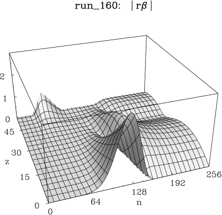
Figure 8: Evolution of $r\beta$ for $0\leq z\leq 55$, in radial in-falling coordinates. Observe that the in-falling grid tracks the dynamical evolution. This simulation has timestep $\Delta z=0.05$, $n=0$ is the past horizon $r=2\textsc{M}$ and $n=256$ represents future null infinity $\mathcal{I}^{+}$.

4.3 Hypersurface equations

The hypersurface equations are solved by treating them as a large system of ordinary differential equations, with the radial grid coordinate $n$ playing the role of independent variable, and the dependent variables being the values taken by the fields $(H,J,Q,K)$ at the $N^{2}/2$ points of the $(\vartheta,\varphi)$-grid.

The form (30–33) of the hypersurface equations, for the variables $\log H$, $rQ^{+}$, $j$ and $K$, proves to be better behaved near $r=\infty$, since each of these variables has a finite (usually non-zero) limit. Integration of these radial ODEs is possible up to and including the final point $n=n_{\infty}$, with results whose numerical effectiveness may be seen by inspecting the field values in a neighbourhood of null infinity [9]. Tests described in the following section, in particular the consistency of the constraint equations and the accuracy of the Trautman-Bondi mass decay formula (Figure 17) also confirm that asymptotic behaviour has been reliably calculated.

Note that unlike methods based on Bondi-Sachs or Newman-Unti coordinates [28, 37], integration along the $r$-coordinate lines does not correspond to integrating along the radial null geodesics (the characteristics of the Einstein equations), since in general the NQS shear $\beta$ is non-zero, and the null direction is $\ell=\partial/\partial r-r^{-1}\beta$.

The radial integration with respect to the coordinate $n$ is performed using an 8th order Runge-Kutta scheme [46], with RK step size $\Delta n=1$. The RK8 method requires 13 derivative evaluations per RK step, of which 10 are at intermediate points not on the radial grid. Values of the field $\beta$ and its angular derivatives at these intermediate points are provided by convolution splines generated using the kernel $\phi_{9}$ with samples at integer $n$.

4.4 Reconstructing the metric

Step 4 of the solution algorithm requires us to reconstruct the metric functions $(u,v,\gamma)$ from the solution $(H,J,K,Q)$ of the hypersurface system (22–25) with seed $\beta$ and boundary data $(H,J,K,Q)|_{r=r_{0}}$. Note that the connection variables (10–14) are determined by the values of the metric functions $(\beta,\gamma,u,v)$ and $\partial\beta/\partial z$ on the hypersurface $\mathcal{N}_{z}$.

The reconstruction is carried out as described in section 2.3. This process requires solving the system (16) on each $S^{2}$ of the radial grid. If $\beta$ is not too large, then (16) is an elliptic system of partial differential equations on the sphere $S^{2}$, mapping surjectively to the space of spin 2 fields. We solve (16) by first substituting

$$\gamma=\eth^{-1}\Gamma,$$ (74)

where $\eth^{-1}$ is defined spectrally by

$$\eth^{-1}Y^{2}_{lm}=-\left[{\textstyle{\frac{1}{2}}}(l+2)(l-1)\right]^{-1/2}Y^{1}_{lm},\quad l\geq 2,$$

so (16) becomes

$$\mathcal{K}_{\beta}\Gamma:=\Gamma+\frac{\eth\beta}{2-{\mbox{div}}\beta}{\mbox{div}}(\eth^{-1}\Gamma)\;=\;-K+J\frac{\eth\beta}{2-{\mbox{div}}\beta}\,.$$ (75)

Note that the choice (74) gauges the $l=1$ spherical harmonic components of $\gamma$ to zero — a similar but more expensive construction may be used if nonzero $\gamma_{l=1}$ components are desired. The advantage of (75) over (16) is that the operator $\mathcal{K}_{\beta}$ in (75) is close to the identity for small $B:=\eth\beta/(2-{\mbox{div}}\beta)$. The corresponding discretized problem is therefore well suited to iterative matrix methods.

We use the conjugate gradient (CG) method [33], which is an iterative method applicable to matrix problems of the form $Ax=b$ with $A$ symmetric positive definite. Accordingly we actually solve an associated self-adjoint equation obtained by applying to (75) the operator adjoint to that in (75) with respect to the $L^{2}$ norm on $S^{2}$.

In order to compute the adjoint operator $\mathcal{K}_{\beta}^{T}$, notice first that $\mathcal{L}_{\beta}$ and $\mathcal{K}_{\beta}$ are real-linear but not complex-linear, so the adjoint must be computed with respect to the real form of the inner product (46). Expanding $\Gamma=\sum_{l\geq 2}\Gamma^{lm}Y^{2}_{lm}$, $\phi=\sum_{l\geq 1}\phi^{lm}Y^{1}_{lm}$ we have the spectral representations

$$\eth^{-1}\Gamma = -\sum_{l\geq 2,m}\left[{\textstyle{\frac{1}{2}}}(l-1)(l+2)\right]^{-1/2}\Gamma^{lm}Y^{1}_{lm},$$ (76)

$${\mbox{div}}\phi = \sum_{l\geq 1,m}\left[{\textstyle{\frac{1}{2}}}l(l+1)\right]^{1/2}(\phi^{lm}+\bar{\phi}^{lm})Y_{lm},$$ (77)

and thus the real adjoints $(\eth^{-1})^{T}$, ${\mbox{div}}^{T}$ are

$$\eth^{-1T}\phi = -\sum_{l\geq 2,m}\left[{\textstyle{\frac{1}{2}}}(l+2)(l-1)\right]^{-1/2}\phi^{lm}Y^{2}_{lm},$$ (78)

$${\mbox{div}}^{T}(f+{\rm i}\,g) = 2\sum_{l\geq 1,m}\left[{\textstyle{\frac{1}{2}}}l(l+1)\right]^{1/2}f^{lm}Y^{1}_{lm},$$ (79)

where $f,g$ are real-valued functions. Consequently we may represent the adjoint $\mathcal{K}_{\beta}^{T}$ spectrally by

$$(\mathcal{K}_{\beta}^{T}\phi)^{lm}=\phi^{lm}-\sqrt{\frac{l(l+1)}{(l-1)(l+2)}}(\bar{B}\phi+B\bar{\phi})^{lm},$$ (80)

where $B=\eth\beta/(2-{\mbox{div}}\beta)$ and $l\geq 2$.

The equation (16) transformed into (75) gives an invertible equation

$$\mathcal{A}_{\beta}\Gamma:=\mathcal{K}_{\beta}^{T}\mathcal{K}_{\beta}\Gamma=\mathcal{K}_{\beta}^{T}(JB-K).$$ (81)

The right hand side of (81) may be computed explicitly using the spectral representation and (80). The operator $\mathcal{A}_{\beta}$ is symmetric and positive definite and close to the identity when considered in the spectral representation. Thus the conjugate gradient algorithm may be applied to (81) and we see that the parameterisation of (16) in terms of $\Gamma$ (74) amounts to a preconditioner. Note CG requires not that the matrix of $\mathcal{A}_{\beta}$ be given explicitly, but only that $\mathcal{A}_{\beta}\Phi$ can be evaluated for any spin 2 field $\Phi$. We carry out this evaluation by a sequential process which computes the actions of $\mathcal{K}_{\beta}$ and $\mathcal{K}_{\beta}^{T}$ using the spectral representations of $\eth^{-1},\eth^{-1T}$ and ${\mbox{div}},{\mbox{div}}^{T}$ (which are simple diagonal operators) combined with transformations to the point representation to evaluate multiplication terms like $\bar{B}\Phi$ followed by projections back to the spectral representation.

This scheme requires several transformations between representations of fields by their spin-weighted spherical harmonic coefficients and by their values on the $S^{2}$ grid. For example, the operator $\eth^{-1}$ is a trivial multiplicative operator on spectral coefficients, whereas the products in the source terms are best calculated in the grid representation. Although evaluating the action of $\mathcal{A}_{\beta}$ is thus numerically expensive, the expense is more than compensated for by the rapid convergence of the CG algorithm with this spectral preconditioning.

The spectral representation has the further advantages that the solution is represented fewer unknowns ($2(L+1)^{2}-8$ compared to $4(L+1)^{2}$ for the grid value representation), and gauge conditions which specify the $l=1$ components of $\gamma$ (eg. $\gamma_{l=1}=0$) can be directly implemented. It is possible to adapt the algorithm to allow for other NQS gauges (eg. $\beta_{l=1}=0$), but this is numerically more expensive since (16) must be solved 4 times at each sphere rather than once. Although such gauges have some geometric advantages [7], their numerical implementation has not yet been considered.

Using CG to solve for the spin 2 spherical harmonic coefficients of $\Gamma$ turns out to be quite efficient, typically requiring fewer than 10 iterations for an $S^{2}$ grid of size $N/2\times N=16\times 32$. On this size grid we resolve all components of $\Gamma$ up to angular momentum $L=N/2-1=15,$ so in this case we are solving for $2((L+1)^{2}-4)=504$ spectral coefficients. The scheme’s effectiveness is due in part to having a good initial guess for $\Gamma$ to use as the starting point of the CG iterations, namely the solution found for $\Gamma$ on the 2-sphere at the previous radial position.

The CG iterations finish when the error, measured by the sum of squares of spherical harmonic coefficients of the difference of the two sides of (75), is $10^{-2}$ times the size of the aliasing error in the source term. This aliasing error is the difference between the raw field values of the source term (which is necessarily calculated in the field value representation because it involves products and quotients) and its field values after projection into the subspace spanned by spin 2 spherical harmonics. It provides an estimate of the error in the source term, and hence (because the operator $\mathcal{K}_{\beta}$ is close to the identity) it is reasonable to accept a solution of comparable accuracy.

To ensure termination of the CG algorithm, other stopping criteria are also checked, but the relative error test is the usual termination cause and is found to work well in practice. For example, it can result in a 10-fold improvement over letting the CG iterations run until the solution is determined to machine precision.

4.5 Evolution

Given $\beta$ on a null hypersurface $\mathcal{N}_{z}$, we construct the time derivative $\partial\beta/\partial z$ by solving the hypersurface equations with seed $\beta$, determining $\gamma,v$ as outlined in the previous section, and then using formula (18) to evaluate $\partial\beta/\partial z$. Let us write the result of this process as

$$\frac{\partial\beta}{\partial z}=\mathcal{B}(\beta,U_{0})$$ (82)

where the operator $\mathcal{B}$ is determined by the value of $\beta$ on the hypersurface $\mathcal{N}$ and the initial conditions $U_{0}=(H_{0},Q_{0},J_{0},K_{0})$ at $r=r_{0}$ for the hypersurface equations.

The evolution formula (82) provides the basis of the spacetime evolution algorithm, which simply incorporates (82) into a standard 4th order Runge-Kutta algorithm. This approach is just the method of lines, treating the evolution equations as a very large system of ordinary differential equations for the (point) representation of the entire field $\beta(z)=\beta_{|\mathcal{N}_{z}}$.

The method of lines, applied blindly in this manner, is generally prone to instabilities. Tests suggest the relative stability of the NQS code derives from the smoothing effects (a) of the convolution spline, and (b) of the spectral projection. The filtering implicit in the convolution spline is applied to $\beta$ during the radial integration of the hypersurface equations, at each of the 4 stages of the RK4 algorithm. It is not possible to turn off this radial filtering because the convolution splines for $\beta$ are an essential part of the algorithm for evaluating the right hand side of (82).

Smoothing of $\beta$ in the angular directions is done explicitly, by projecting $\beta$ onto the spin 1 subspace with maximum angular momentum $L$ or $2L/3$ (the Orszag $2/3$ rule, to eliminate quadratic aliasing). This angular filtering is done after each of the 4 stages of the RK4 algorithm. Removal of the angular filtering results in very rapid disintegration of the evolution, which then typically lasts only a few RK4 steps.

For simplicity, the 4 RK4 stages evolve $\beta$ in the $z$ direction in the $(z,r)$ coordinates, along $r=const$. At the end of each full RK4 time step the key field $\beta$ is interpolated onto the new radial grid (72), using a convolution spline based on values of $\beta$ on the old grid.

The RK4 time integration of $\beta$ evolves field values on the $(\vartheta,\varphi)$-grid. Equivalently, we could have evolved its spherical harmonic coefficients, of which there are only half as many. However, the amount of computation saved by doing so is insignificant in comparison to that required to evaluate $\partial\beta/\partial z$, so this choice is made for convenience.

Likewise, the RK8 radial integration of the system of hypersurface equations uses the field value representation. In this case, however, it is found that projecting the fields onto their appropriate spherical harmonic subspaces during the integration is not required for either stability or accuracy. There is a definite computational advantage in staying within the field value representation, since several relatively expensive $O(L^{3})$ projections are avoided.

The first radial derivative of $\gamma$ is needed to evaluate $\partial\beta/\partial z$ (18). Grid values of $\partial\gamma/\partial r$ are calculated numerically as derivatives of convolution splines (in the radial direction) for the $(\vartheta,\varphi)$-grid values of $\gamma$, making use of formula (73) and the chain rule for derivatives. The radial derivative term $\mathcal{D}_{r}\log u$ appears in the hypersurface equations (31) and (32). Using equation (30) and definition (15), this term can be written as an expression involving only the 1st radial and angular derivatives of $\beta$.

The program is normally run until the solution ceases to be well behaved. Blowup is detected by monitoring $2-{\mbox{div}}\beta$, which must remain everywhere positive. For the initial data that we have used, the blowup has always occurred in the $l=2$ modes of $\beta$, at low values of $n$ corresponding to $r-2\textsc{M}\approx 0$ (see Figures 7,8). Although the precise cause of the blowup is not yet understood, it is not a numerical instability, since it is unaffected by changes in the radial or timestep resolutions, nor does it appear to be primarily geometric, since most curvature scalars remain bounded. This suggests the blowup is a coordinate effect, probably arising from proximity to the future event horizon.

For smooth initial data of intermediate strength (run_160), the evolution extends to $z\sim 55$. The final time varies with the strength of the initial data — see Table 3. The evolution of an intermediate strength solution is shown in Figure 8, which plots the mean square or $L^{2}(S^{2})$ size of $\beta$ at each radial sphere, for time $0\leq z\leq 55$. Termination is caused by the blowup feature at low radius, which grows steadily from time $z=40$ onwards.

5 Accuracy tests

The complexity of the NQS Einstein equations and the variety of algorithms employed in the code, make it problematic to prove rigorously that the numerical simulation accurately models the physics and geometry of the spacetime. Instead we rely on a range of tests to justify the reliability of the code, probing the numerical accuracy of the solutions through their convergence and geometric consistency.

We consider here tests based on the numerical convergence of the solutions as algorithmic parameters are varied; and on the algebraic consistency of the numerical solutions. The consistency tests measure the constraint identities and the Trautman-Bondi mass decay formula [63, 28]. Work in progress considers other tests, including comparisons with linearised theory, and with better known solutions such as Robinson-Trautman, Schwarzschild and Minkowski spacetimes in twisted NQS coordinates [7].

The resolution of the simulations is determined by three parameters: the spherical harmonic spectral limit $L$ (or effective limit $l_{\rm max}$); the number of radial zones $n_{\infty}$; and the time step $\Delta z$. We shall examine in turn how the accuracy of a solution depends on each of these parameters.

It is clear that numerical convergence can be estimated from the convergence properties of the key field $\beta$. However, convergence of $\beta$ guarantees only that the (limit) solution satisfies some system of equations, which may not coincide with the desired vacuum Einstein equations. (For example, the Einstein equations may have been incorrectly implemented). Thus, to assert that the correct equations have been solved, it is essential to provide independent tests of the correctness of the code.

The most natural independent test is to compare the numerical solution with an explicitly known solution. Unfortunately the Schwarzschild metric (4) is trivial in the NQS gauge and does not provide a useful comparison test, whilst the twisted shear-free metrics [7] require boundary conditions which are more general than those available in the present version of the code.

Instead we consider here another class of independent tests based on constraint relations. Such relations are typical of geometric equations arising in geometry and physics, which admit gauge and coordinate freedoms. Thus, we check the geometric consistency of the solution by evaluating $r^{2}G_{nn}$ and $r^{2}G_{nm}$, using the constraint relations (26) and (27). Neither of these relations is used in generating the numerical solutions, and in theory these components should evaluate to zero. In practice, since each is a sum of terms having magnitude approximately $|\beta|\sim 1$, the extent to which $r^{2}G_{nn}$, $r^{2}G_{nm}$ evaluate to zero serves both to confirm the consistency of the numerical solution with the vacuum Einstein equations, and also to assess the accuracy of the solution.

The Trautman-Bondi mass decay formula provides another such test of geometric consistency, and of the accuracy of the solution near $r=\infty$. This theoretical result leads to a relation between the asymptotic ($r=\infty$) values and $z$-derivatives of the fields $H$, $J$, and $K$, and may be readily tested for our numerical solutions.

In the following we discuss numerical solutions using three reference initial $\beta(z=0)$ fields, which differ only by the scale factors given in Table 3. In each case the initial $\beta$ consists of pure $l=2,m=2$ spherical harmonics with equal strength odd and even parts, and radial profile given by a bump supported on $5\leq r\leq 40$. We use the terms weak, intermediate and strong to describe solutions generated using the three sizes of initial data.

Another convenient measure of the strength of the gravitational field is the initial relative mass difference $m_{B}(0)/\textsc{M}-1$, between the initial Bondi mass of the numerical spacetime (cf. (85)) and the background Schwarzschild mass (M). Table 3 gives the initial relative mass differences for the three reference initial $\beta$ fields.

Table 3: Size of initial data sets

Field strength:	weak	intermediate	strong
$\beta(0)$ scale factor:	1	4.48	10
$m_{B}(0)/\textsc{M}-1$:	$0.9472\times 10^{-2}$	$0.1915$	$0.9940$
Last $z$:	61	55	51

The qualitative conclusions of the error analysis of this section may be summarised as follows:

The major determining factor in the overall accuracy is the spectral limit $L$. Truncating spherical harmonic coefficients beyond $L$ has the effect of modifying the Einstein equations to a system for which the constraint identities are no longer valid, and thereby places a lower bound on the numerical accuracy. For $L=15$ the weak and intermediate field solutions can be adequately resolved, but this is not sufficient to obtain adequate (beyond $10^{-3}$) accuracy for the strong field simulation run_170.

To suppress unstable quadratic aliasing effects, it is essential to use an Orszag 2/3 rule truncation.

Within the bounds governed by the spectral limit $L$, accuracy can be improved by increasing the radial resolution $n_{\infty}$. For the weak field solution, $n_{\infty}=1024$ reduces the radial error contribution to the level of the spectral truncation error (see Figure 14(b)).

For given resolutions $L$ and $n_{\infty}$, there is a range of values $\Delta z$ for which the simulation remains stable. Outside this range, the simulation follows the standard solution for some time, then rapidly blows up. The simulation is largely insensitive to the value of $\Delta z$ within the stable range, so $\Delta z$ may be chosen as large as possible, consistent with stable evolution.

5.1 Dependence on spectral limit $L$

Using our current hardware it is not generally feasible to run the code at $L=31$, and $L=7$ is too low to be of interest. The code is normally run at $L=15$ resolution (giving a $16\times 32$ $(\vartheta,\varphi)$ grid) with an anti-aliasing cutoff at $l_{\rm max}=10$.

Orszag [18, 41] observed that quadratic aliasing can be eliminated by periodically removing the upper $1/3$ of the spectral bandwidth of a numerical solution. If fields contain only modes for which $l\leq\frac{2}{3}L$, then a quadratic product is band limited to $l\leq\frac{4}{3}L$. With a working bandwidth $L$, the modes for which $L\leq l\leq\frac{4}{3}L$ become aliased onto the modes $\frac{2}{3}L\leq l\leq L$. Therefore, truncation at $l_{\rm max}=\frac{2}{3}L$ will remove quadratic aliasing contamination.

If no cutoff is used (ie. the full $L=15$ resolution is retained) then the high $l$-modes of the intermediate strength simulations blow up at $z\approx 8$. The onset of instability (time until blow up) of the $L=15$ simulations with no $l_{\rm max}$ cutoff is largely independent of the time step and the radial resolution. This suggests that the effect of the nonlinear aliasing contamination is best regarded as changing the system of equations into a system which has unstable solutions.

Because the nonlinear interactions in the NQS equations are predominantly quadratic, it is not surprising that the $l_{\rm max}=10$ cutoff is sufficient for long term stability. The intermediate strength solution lasts until $z=55$, when the code terminates for other reasons.

Figure 9(a) shows blow up of run_453, an $L=15$ simulation of the intermediate field strength solution. The $l=15$ modes show rapid growth beyond $z=6$, indicating the instability of the aliasing feedback. Figure 9(b) shows the difference between run_453 and the stable simulation run_456, which has an $l_{\rm max}=10$ cutoff. Until the onset of the high $l$-mode instability (ie. for $z\leq 6$) there is good agreement between the two simulations, with approximately $10^{-10}$ relative difference for $l=2$ modes and $10^{-2}$ relative difference for $l=10$ modes.

(a) (b)

Figure 9: Orszag’s $2/3$ rule is used to remove aliasing instability: (a) unstable evolution of the high $l$-modes of an $L=15$ simulation (no anti-aliasing cutoff); (b) difference between an unstable $L=15$ simulation (no cutoff) and a stable simulation with an $l_{\rm max}=10$ cutoff. Each $l$-bin contains a radial plot (linear in $n$, with $n=0,\ldots,n_{\infty}$) of the square root of the sum of the squares of the $(l,m)$-components for fixed $l$ with $m=-l,\ldots,l$. These simulations have $n_{\infty}=512$ and $\Delta z=0.05$.

The spectral limit $L$ is critical in determining the relation between gravitational field strength and simulation accuracy. This can be appreciated by observing the decay rate of the $l$-spectrum of $\beta$, as in Figure 10. By extrapolation, the error introduced by the anti-aliasing cutoff at $l_{\rm max}=10$ should be no more than the $l=10$ coefficient, and a relative error estimate follows by comparing the $l=10$ and the $l=2$ coefficients.

Figures 10(a) and 10(b) show the dramatic difference in decay rates of the $l$-modes of $\beta$ for weak and strong fields. Assuming an $l_{\rm max}=10$ cutoff, it is evident that the relative error is at most $10^{-8}$ for weak field simulations, and about $10^{-3}$ for strong field simulations.

(a) (b)

Figure 10: Spectral resolution and field strength: (a) well resolved weak field with fast $l$-mode decay; (b) poorly resolved strong field with slow decay of $l$-modes (see Table 3 for field strength details).

From the observed decay rate of the $l$-modes of $\beta$ for a given field strength, it is possible to estimate the resolution $L$ required to achieve a prescribed accuracy. Thus although we cannot directly investigate the behaviour of errors with varying spectral limit $L$ (due to hardware constraints), we can still investigate spectral resolution effects by altering the $\beta$ field strength.

Figures 11(a) and 11(b) show the effect of field strength (weak, intermediate, strong) on the constraint quantities $r^{2}G_{nn}$ and $r^{2}G_{nm}$. The parameters for these simulations are $l_{\rm max}=10$, $n_{\infty}=256$ and $\Delta z=0.05$. The four curves in each band are times $z=10,20,30,40$. There is no significant $z$ dependence of either $G_{nn}$ or $G_{nm}$ until within about $5\textsc{M}$ of the final blow up time.

(a) (b)

Figure 11: Effect of spectral resolution on constraint quantities (a) $|r^{2}G_{nn}|_{S^{2}}$; (b) $|r^{2}G_{nm}|_{S^{2}}$, at times $z=10,20,30,40$, for strong (top 4 curves), intermediate (middle 4 curves) and weak (bottom 4 curves) fields.

The second Bianchi identity implies the conservation law $G_{ab}^{;b}=0$, which leads to a radial system of equations for $G_{nn},G_{nm}$ with sources linear in the hypersurface Einstein tensor components $G_{\ell\ell}$, $G_{\ell m}$, $G_{\ell n}$, $G_{mm}$. Thus $G_{nn},G_{nm}$ give a measure of the accumulated error in the hypersurface equations in the radial direction. This provides some explanation of the structure of the $G_{nn},G_{nm}$ graphs, particularly for the strong field solution: the numerical solution of the hypersurface equations will have greatest error in the region where the fields are strongest, in this case the range $64<n<128$, and this is precisely the region of greatest increase in $G_{nn},G_{nm}$.

5.2 Dependence on radial grid resolution $n_{\infty}$

The radial regridding and interpolation of $\beta$, the radial differentiation of $\gamma$, and the RK integration of the hypersurface equations are all formally 8th order accurate. Figure 12 shows that this is consistent with the observed convergence of $\beta$ on increasing the radial resolution.

Figure 12: Convergence of $\beta$ with increasing radial resolution: weak field solutions with $n_{\infty}=256,512$ compared to $n_{\infty}=1024$. The error decreases by approximately a factor of $2^{8}$ on doubling the radial resolution.

The constraint quantities $G_{nn}$ and $G_{nm}$ also exhibit some convergence effects. Figures 13(a) and 13(b) show show significant improvement between $n_{\infty}=256$ and $512$, but little between $512$ and $1024$. The form of the $n_{\infty}=1024$ curve indicates that errors at the highest radial resolution are dominated by errors associated with the spectral truncation.

(a) (b)

Figure 13: Effect of radial resolution on weak field constraint quantities (a) $|r^{2}G_{nn}|_{S^{2}}$, (b) $|r^{2}G_{nm}|_{S^{2}}$. In each case the three curves are $n_{\infty}=256,512,1024$ (top, middle and bottom curves respectively).

5.3 Dependence on time step $\Delta z$

Although the solution algorithm is formally 4th order accurate in the time direction, at the typical resolutions at which the code is run, the RK4 errors are completely dominated by errors arising from the spectral truncation $L$ and/or the radial discretisation $n_{\infty}$. This is illustrated by Figure 14(a), which shows no significant difference in the constraint quantity $G_{nn}$ between $\Delta z=0.1$ and $\Delta z=0.05$, with $n_{\infty}=256$. However, when the solution is better resolved in the radial direction, a small effect can be observed, cf. Figure 14(b), where $n_{\infty}=1024$. Figure 15 compares $r\beta$ for runs with $\Delta z=0.1,0.05,0.025$ and $n_{\infty}=512$ and again shows only minor improvements from decreasing $\Delta z$.

(a) (b)

Figure 14: Effect of time step resolution on the constraint quantity $|r^{2}G_{nn}|_{S^{2}}$ for the weak field solution: (a) $n_{\infty}=256,\Delta z=0.1,0.05$: the error is dominated by the radial discretisation error for $n<192$ and by the spectral truncation error for $n>192$. Refining $\Delta z$ produces no appreciable improvement in the solution. (b) $n_{\infty}=1024,\Delta z=0.1,0.05$: the radial discretisation error is small enough that the RK4 integration error can be observed. For $n>700$ the error is dominated by the spectral truncation, resulting in the same tail as in (a), while for $n<700$ the constraint improves in places, consistent with a factor of 16 decrease in the error.

Figure 15: Convergence of $\beta$ with decreasing time step: weak field solutions for $\Delta z=0.1,0.05$, compared against $\Delta z=0.025$. Where the error is not dominated by the radial discretisation error, the curves show a decrease in error which is consistent with 4th order convergence.

Consequently, $\Delta z$ is optimally chosen as large as possible, subject to resulting in stable evolution. For $n_{\infty}=256$ and $L=15$ with an anti-aliasing $l_{\rm max}=10$ cutoff, the evolution is stable for $\Delta z=0.1$ and unstable for $\Delta z=0.2$, which blows up at time $z=25$, after 125 RK4 steps.

5.4 Energy and asymptotic decay tests

The Hawking mass

$$m_{H}(\Sigma)=\sqrt{\frac{\textrm{area}(\Sigma)}{16\pi}}\left(1-\frac{1}{2\pi}\oint_{\Sigma}\rho_{NP}\mu_{NP}\,dv_{\Sigma}\right)$$ (83)

of a 2-surface $\Sigma$ reduces in the NQS gauge to

$$m_{H}(z,r)={\textstyle{\frac{1}{2}}}r\left(1-\frac{1}{8\pi}\oint_{S^{2}}HJ\right).$$ (84)

$m_{H}(z,r)$ provides an easily computed quantity representing the “quasi-local” mass contained within the sphere $(z,r)$, and has asymptotic limit equal to the Bondi mass

$$m_{B}(z)=\lim_{r\to\infty}m_{H}(r,z).$$ (85)

The Bondi mass is easily computed numerically, by $m_{B}(z)=m_{H}(n=n_{\infty},z)$. Figure 16(a) shows the Hawking mass plotted against the radial coordinate, for times $z=0,1,\ldots,60$. There are several features of interest in this plot: the limit Bondi mass (Figure 16(b)) decays in time, reflecting the Trautman-Bondi mass loss formula (86); the energy is radiated in bursts, reflecting near-linear behaviour dominated by pure $l=2$ modes; the Hawking and Bondi masses decay to background black hole mass $\textsc{M}=1$ at late times, suggesting that in this example, almost all the gravitational radiation has been scattered to $\mathcal{I}^{+}$ and essentially none will be absorbed by the black hole; and finally, the rapidly growing feature about $n=20$ at late times in Figure 8, does not affect the Hawking mass.

The Trautman-Bondi mass loss formula [62, 63, 14, 28]

$$\frac{d}{dz}m_{B}(z)={}-\frac{1}{16\pi}\lim_{r\to\infty}\oint_{S^{2}(z,r)}H|K|^{2}.$$ (86)

provides another test of the geometric consistency of the solution, particularly near null infinity. By comparing the numerical derivative $dm_{B}/dz$ with the computed value of the right hand side (evaluated at $n=n_{\infty}$), we may construct the error $\frac{d}{dz}m_{B}-\textrm{RHS(\ref{eq:dzmB})}$. Figure 17(b) plots this error against time $z$, suggesting that the asymptotic ($r=\infty$) fields of run_160 are accurate to about $0.00001\%$.

(a) (b)

Figure 16: Mass functions: (a) Hawking mass for times $z=0,1,\ldots,55$; (b) Bondi mass.

(a) (b)

Figure 17: The Trautman-Bondi mass loss formula as test of numerical accuracy at $r=\infty$: (a) Bondi mass decay rate; (b) error in the mass decay formula, given by ${\rm LHS(\ref{eq:dzmB})}-{\rm RHS(\ref{eq:dzmB})}$.

References

- [1] S. Abarbanel, D. Gottlieb, and M. H. Carpenter. On the removal of boundary errors caused by Runge-Kutta integration of nonlinear partial differential equations. SIAM J. Sci. Comp., 17:777–782, 1996.
- [2] R. Balean. The null-timelike boundary problem for the linear wave equation. PhD thesis, University of New England, 1996.
- [3] R. Balean. The null-timelike boundary problem for the linear wave equation. Commun. P.D.E., 22:1325–1360, 1997.
- [4] R. Bartnik. Quasi-spherical metrics and prescribed scalar curvature. J. Diff. Geom., 37:31–71, 1993.
- [5] R. Bartnik. Einstein equations in the null quasi-spherical gauge. Class. Quant. Gravity, 14:2185–2194, 1997.
- [6] R. Bartnik. Einstein equations in the null quasi-spherical gauge: progress report. In D. Wiltshire, editor, ACGRG1 Proceedings, Adelaide February 1996, pages 25–38, 1997. http://www.physics.adelaide.edu.au/ASGRG/ACGRG1/.
- [7] R. Bartnik. Shear-free null quasi-spherical spacetimes. J. Math. Phys., 38:5774–5791, 1997.
- [8] R. Bartnik. Interaction of gravitational waves with a black hole. In T. Bracken and D. De Wit, editors, Proceedings, XIIth Int’l. Congress Math. Phys., Brisbane, July 1997. International Press, to appear 1999.
-
[9]
R. Bartnik and A. H. Norton.
NQS data explorer.
Technical report, University of Canberra, 1997.
http://gular.canberra.edu.au/relativity.html. - [10] R. Bartnik and A. H. Norton. Numerical solution of the Einstein equations. In A. Gill J. Noye, M. Teubner, editor, Computational Techniques and Applications: CTAC97, pages 91–98, 1998.
- [11] N. Bishop, R. Gómez, L. Lehner, M. Maharaj, and J. Winicour. High-powered gravitational news. Phys. Rev. D, 56:6298, 1997.
- [12] N. T. Bishop. Some aspects of the characeristic initial value problem in numerical relativity. In C. J. Clarke and R. d’Inverno, editors, Prospects in Numerical Relativity II, pages 20–33. Cambridge, 1992.
- [13] S. Bonazzola, E. Gourgoulhon, and J.-A. Marck. Spectral methods in general relativistic astrophysics. gr-qc/9811089, 1998.
- [14] H. Bondi. Gravitational waves in general relativity. Nature, 186:535, 1960.
- [15] J. P. Boyd. The choice of spectral functions on a sphere for boundary and eigenvalue problems: A comparison of Chebyshev, Fourier and asssociated Legendre expansions. Mon. Weather Rev., 106:1184–1191, 1978.
- [16] J. P. Boyd. Chebyshev and Fourier Spectral Methods. Lecture Notes in Engineering, vol 49. Springer, 1989.
- [17] G. L. Browning, J. J. Hack, and P. N. Swarztrauber. A comparison of three numerical methods for solving differential equations on the sphere. Mon. Weather Rev., 117:1058–1075, 1989.
- [18] C. Canuto, M. Y. Hussaini, A. Quarteroni, and T. A. Zang. Spectral Methods in Fluid Mechanics. Series in Computational Physics. Springer, 1988.
- [19] S. Chandrasekhar. The Mathematical Theory of Black Holes. Oxford, 1984.
- [20] R. D’Inverno. Introducing Einstein’s Relativity. Oxford, 1992.
- [21] M. Eastwood and P. Tod. Edth – a differential operator on the sphere. Math. Proc. Camb. Phil. Soc., 92:317–330, 1982.
- [22] J.A.H. Futterman, F.A. Handler, and R.A. Matzner. Scattering from black holes. Cambridge, 1988.
- [23] J. N. Goldberg, A. J. Macfarlane, E. T. Newman, F. Rohrlich, and E. C. G. Sudarshan. Spin- spherical harmonics and . J. Math. Phys., 8:2155–2161, 1967.
- [24] R. Gómez, P. Papadopoulos, and J. Winicour. Null cone evolution of axi-symmetric vacuum space-times. J. Math. Phys., 35:4184–4203, 1994.
- [25] R. Gómez and J. Winicour. Asymptotics of gravitational collapse of scalar waves. J. Math. Phys., 33:1445, 1992.
- [26] R. Gómez, J. Winicour, and R. Isaacson. Evolution of scalar fields from characteristic data. J. Comp. Phys., 98:11, 1992.
- [27] R. Gómez, J. Winicour, and P. Papadopoulos. The eth formalism in numerical relativity. Class. Quantum Grav., 14:977–990, 1997.
- [28] M. G. J. van der Berg H. Bondi and A. W. K. Metzner. Gravitational waves in general relativity VII. Proc. Roy. Soc. Lond., A269:21–51, 1962.
- [29] R. W. Hamming. Digital Filters. Prentice-Hall, 1977.
- [30] S. W. Hawking and G. R. Ellis. The large-scale structure of spacetime. Cambridge UP, Cambridge, 1973.
- [31] A. C. Hearn. REDUCE Users Manual, Version 3.6. RAND Publication CP78 (rev. 9/96), 1996.
- [32] R. Jakob-Chien and B. K. Alpert. A fast spherical filter with uniform resolution. J. Comp. Phys., 136:580–584, 1997.
- [33] C. Johnson. Numerical Solution of Partial Differential Equations by the Finite Element Method. Cambridge, 1987.
- [34] P. E. Merilees. The pseudo-spectral approximation applied to the shallow water equations on a sphere. Atmosphere, 11:13–20, 1973.
- [35] V. Moncrief. Gravitational perturbations of spherically symmetric systems. Ann. Phys., 88:323–342, 1974.
- [36] E. Newman and R. Penrose. An approach to gravitational radiation by a method of spin coefficients. J. Math. Phys., 3:566–578, 1962.
- [37] E. T. Newman and T. Unti. A class of null flat-spce coordinate systems. J. Math. Phys., 4:1467–1469, 1963.
- [38] A. H. Norton. Finite difference operators for pdes, based on sampling kernels for spline quasi-interpolation. Technical report, School of Mathematics, UNSW, 1992.
- [39] A. H. Norton. Spectral collocation methods for solution of Einstein’s equations in null quasi-spherical coordinates. In D. L. Wiltshire, editor, Proceedings of the First Australasian Conference on General Relativity, Adelaide February 1996, pages 39–47, 1997. http://www.physics.adelaide.edu.au/ASGRG/ACGRG1/.
- [40] A. H. Norton. The use of convolution splines in the NQS Einstein evolution code. In A. Gill J. Noye, M. Teubner, editor, Computational Techniques and Applications: CTAC97, pages 473–480, 1998.
- [41] S. A. Orszag. On the elimination of aliasing in finite difference schemes by filtering high wave number components. J. Atmosph. Sci., 28:1074, 1971.
- [42] S. A. Orszag. Fourier series on spheres. Monthly Weather Rev, 102:56–75, 1974.
- [43] R. Penrose. The geometry of impulsive gravitational waves. In L. O’Raifaertaigh, editor, General Relativity: in honour of J.L.Synge. Oxford, 1972.
- [44] R. Penrose and W. Rindler. Spinors and Space-time, vol. I,II. Cambridge UP, 1984,1986.
- [45] D. A. Prager and A. W. C. Lun. Computational methods in the physical interpretation of Robinson-Trautman spacetimes. In D. L. Wiltshire, editor, First Australasian Conference on General Relativity and Gravitation, 1996.
- [46] P. J. Prince and J. R. Dormand. High order embedded Runge-Kutta formulae. J. Comp. Appl. Math., 7:67–75, 1981.
- [47] T. Regge and J. A. Wheeler. Stability of a Schwarzschild singularity. Phys. Rev., 108:1063–1069, 1957.
- [48] A. D. Rendall. Reduction of the characteristic initial value problem to the Cauchy problem and its application to the Einstein equations. Proc. Roy. Soc. Lond., A427:221–239, 1990 MPI preprint 438, 1989.
- [49] I. Robinson and A. Trautman. Spherical gravitational waves in general relativity. Proc. Roy. Soc. Lond. A, 270:103–126, 1962.
- [50] R. K. Sachs. Gravitational waves in general relativity, VIII. waves in asymptotically flat space-time. Proc. Roy. Soc. Lond. A, A270:103–126, 1962.
- [51] R. K. Sachs. Gravitational waves in general relativity VIII. waves in asymptotically flat space-time. Proc. Roy. Soc. Lond., A270:103–126, 1962.
- [52] L. J. Schoenberg. Cardinal Spline Interpolation, volume 12 of Regional Conference Series in Applied Mathematics. SIAM, 1973.
- [53] D. Singleton. Robinson-Trautman solution of Einstein’s equations. PhD thesis, Monash University, 1990.
- [54] L. Smarr and Jr. J. W. York. Kinematical conditions in the construction of spacetime. Phys. Rev. D, 17:2529–2551, 1978.
- [55] G. Starius. Composite mesh difference methods for elliptic and boundary value problems. Numer. Math., 28:243–248, 1977.
- [56] K. Stellmacher. Ausbretungsgesetze für charakteristische Singularitäten der Gravitationsgleichungen. Math. Annalen, 145:740–783, 1938.
- [57] F. Stenger. Numerical Methods Based on Sinc and Analytic Functions. Springer, 1993.
- [58] P. N. Swarztrauber. On the spectral approximation of discrete scalar and vector functions on the sphere. SIAM J. Numer. Anal., 16:934–949, 1979.
- [59] P. N. Swarztrauber. The approximation of vector functions and their derivatives on the sphere. SIAM J. Numer. Anal., 18:191–210, 1981.
- [60] P. N. Swarztrauber. Software for the spectral analysis of scalar and vector functions on the sphere. In Large Scale Scientific Computation. Academic Press, 1984.
- [61] P. N. Swarztrauber. Spectral transform methods for solving the shallow-water equations on the sphere. Mon. Weather Rev,, 124:730, 1996.
- [62] A. Trautman. King’s College lecture notes on general relativity. May-June 1958.
- [63] A. Trautman. Radiation and boundary conditions in the theory of gravitation. Bull. Acad. Pol. Sci., Série sci. math., VI:407–412, 1958.
- [64] A. Trautman. Conservation laws in general relativity. In L. Witten, editor, Gravitation: an introduction to current research. Wiley, 1962.
- [65] F. J. Zerilli. Effective potential for even parity regge-wheeler gravitational perturbation equations. Phys. Rev. Lett., 24:737–738, 1970.
- [66] H. Müller zum Hagen. Characteristic initial value problem for hyperbolic systems of second order differential equations. Ann. Inst. Henri Poincaré, 53:159–216, 1990.