EVOLUTIONARY SEQUENCES OF IRROTATIONAL BINARY NEUTRON STARS

Abstract

We present results of numerical computations of quasiequilibrium sequences of binary neutron stars with zero vorticity, in the general relativistic framework. The Einstein equations are solved under the assumption of a conformally flat spatial 3-metric (Wilson-Mathews approximation). The evolution of the central density of each star is monitored as the orbit shrinks in response to gravitational wave emission. For a compactification ratio $M/R=0.14$, the central density remains rather constant (with a slight increase, below $0.1\%$) before decreasing. For a higher compactification ratio $M/R=0.17$ (i.e. stars closer to the maximum mass configuration), a very small density increase (at most $0.3\%$) is observed before the decrease. This effect remains within the error induced by the conformally flat approximation. It can be thus concluded that no substantial compression of the stars is found, which would have indicated a tendency to individually collapse to black hole prior to merger. Moreover, no turning point has been found in the binding energy or angular momentum along evolutionary sequences, which may indicate that these systems do not have any innermost stable circular orbit (ISCO).

• Département d’Astrophysique Relativiste et de Cosmologie
  UMR 8629 du C.N.R.S., Observatoire de Paris,
  F-92195 Meudon Cedex, France
  Email: Silvano.Bonazzola, Eric.Gourgoulhon, Jean-Alain.Marck@obspm.fr

1 Introduction

Inspiraling neutron star binaries are expected to be among the strongest sources of gravitational radiation that could be detected by the interferometric detectors currently under construction (GEO600, LIGO, TAMA and Virgo). These binary systems are therefore subject to numerous theoretical studies. Among them are (i) Post-Newtonian (PN) analytical treatments (e.g. [1], [2], [3]) and (ii) fully relativistic hydrodynamical treatments, pioneered by the works of Oohara and Nakamura (see e.g. [4]) and Wilson et al. [5, 6]. The most recent numerical calculations, those of Baumgarte et al. [7, 8] and Marronetti et al. [9], rely on the approximations of (i) a quasiequilibrium state and (ii) of synchronized binaries. Whereas the first approximation is well justified before the innermost stable orbit, the second one does not correspond to physical situations, since it has been shown that the gravitational-radiation driven evolution is too rapid for the viscous forces to synchronize the spin of each neutron star with the orbit [10, 11] as they do for ordinary stellar binaries. Rather, the viscosity is negligible and the fluid velocity circulation (with respect to some inertial frame) is conserved in these systems. Provided that the initial spins are not in the millisecond regime, this means that close binary configurations are better approximated by zero vorticity (i.e. irrotational) states than by synchronized states.

Dynamical calculations by Wilson et al. [5, 6] indicate that the neutron stars may individually collapse into a black hole prior to merger. This unexpected result has been called into question by a number of authors (see Ref. [12] for a summary of all the criticisms and their answers). Recently Flanagan [13] has found an error in the analytical formulation used by Wilson et al. [5, 6]. This error may be responsible of the observed radial instability. As argued by Mathews et al. [12], one way to settle this crucial point is to perform computations of relativistic irrotational configurations. We have performed recently such computations [14]. They show no compression of the stars, although the central density decreases much less than in the corotating case. In the present report, we give more details about the results presented in Ref. [14] and extend them to the compactification ratio $M/R=0.17$ (the results of Ref. [14] have been obtained for a compactification ratio $M/R=0.14$).

2 Analytical formulation of the problem

2.1 Basic assumptions

We have proposed a relativistic formulation for quasiequilibrium irrotational binaries [15] as a generalization of the Newtonian formulation presented in Ref. [16]. The method was based on one aspect of irrotational motion, namely the counter-rotation (as measured in the co-orbiting frame) of the fluid with respect to the orbital motion (see also Ref. [17]). Since then, Teukolsky [18] and Shibata [19] gave two formulations based on the definition of irrotationality, which implies that the specific enthalpy times the fluid 4-velocity is the gradient of some scalar field [20] (potential flow). The three formulations are equivalent; however the one given by Teukolsky and by Shibata greatly simplifies the problem. Consequently we used it in the present work.

The irrotational hypothesis amounts to say that the co-momentum density is the gradient of a potential

$$h\,{\bf u}=\nabla\Psi\ ,$$ (1)

where $h$ and $\bf u$ are respectively the fluid specific enthalpy and fluid 4-velocity.

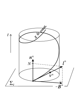
Figure 1: Spacetime foliation $\Sigma_{t}$, helicoidal Killing vector $l^{\alpha}$ and its trajectories $x^{i^{\prime}}={\rm const}$, which are the worldlines of the co-orbiting observer (4-velocity: $v^{\alpha}$). Also shown are the rotating-coordinate shift vector $B^{\alpha}$ and the unit future-directed vector $n^{\alpha}$, normal to the spacelike hypersurface $\Sigma_{t}$ (Figure from Ref. [15]).

Beside the physical assumption (1), two simplifying approximations are introduced:

1. The spacetime is supposed to have a helicoidal symmetry [15], which means that the orbits are exactly circular and that the gravitational radiation content of spacetime is neglected.

2. The spatial 3-metric is assumed to be conformally flat (Wilson-Mathews approximation [21, 5]), so that the full spacetime metric reads

   $$ds^{2}=-(N^{2}-B_{i}B^{i})dt^{2}-2B_{i}dt\,dx^{i}+A^{2}f_{ij}dx^{i}\,dx^{j}\ ,$$ (2)

   where $f_{ij}$ is the flat space metric.

The Killing vector corresponding to hypothesis (i) is denoted by $\bf l$ (cf. Fig. 1).

Approximation (i) is physically well motivated, at least up to the innermost stable orbit. Regarding the second approximation, it is to be noticed that (i) the 1-Post Newtonian (PN) approximation to Einstein equations fits this form, (ii) it is exact for arbitrary relativistic spherical configurations and (iii) it is very accurate for axisymmetric rotating neutron stars [22]. An interesting discussion about some justifications of the Wilson-Mathews approximation may be found in [12]. A stronger justification may be obtained by considering the 2.5-PN metric obtained by Blanchet et al. [23] for point mass binaries. Using Eq. (7.6) of Ref. [23], the deviation from a conformally flat 3-metric (which occurs at the 2-PN order) can be computed at the location of one point mass (i.e. where it is expected to be maximal), the 3-metric $h_{ij}$ being written as

$$h_{ij}=A^{2}\,f_{ij}+h_{ij}^{\rm 2PN}+h_{ij}^{\rm 2.5PN}\ .$$ (3)

The result is shown in Table 1 for two stars of $1.4M_{\odot}$ each. It appears that at a separation as close as $30{\ \rm km}$, where the two stars certainly almost touch each other, the relative deviation from a conformally flat 3-metric is below $2\%$.

$d$	$v/c$	$\omega_{\rm 2PN}$	Conformal fact.	$\left|h_{ij}^{\rm 2PN}\right|/A^{2}$	$\left|h_{ij}^{\rm 2.5PN}\right|/A^{2}$
$\rm[km]$		[rad/s]	$A^{2}$
100	0.10	579	1.04	$1.8\times 10^{-3}$	$6.3\times 10^{-4}$
50	0.13	1572	1.09	$6.8\times 10^{-3}$	$3.3\times 10^{-3}$
40	0.14	2166	1.11	$1.0\times 10^{-2}$	$5.6\times 10^{-3}$
30	0.16	3387	1.15	$1.8\times 10^{-2}$	$1.1\times 10^{-2}$

Table 1: Deviation from a conformally flat 3-metric at 2-PN at 2.5-PN order for point mass binaries of $M=1.4\,M_{\odot}$ each. $d$ is the coordinate separation between the two stars, $v$ is the coordinate orbital velocity of one star, $\omega_{\rm 2PN}$ is the orbital angular velocity, the other notations are defined by Eq. (3). The metric at the 2.5PN level is taken from Blanchet et al. [23] and is computed at the location of the point masses.

2.2 Equations to be solved

We refer to Ref. [14] for the presentation of the partial differential equations (PDEs) which result from the assumptions presented above. In the present report, let us simply mention a point which seems to have been missed by various authors: the existence of the first integral of motion

$$h\,{\bf l}\cdot{\bf u}={\rm const.}$$ (4)

does not result solely from the existence of the helicoidal Killing vector $\bf l$. Indeed, Eq. (4) is not merely the relativistic generalization of the Bernoulli theorem which states that $h\,{\bf l}\cdot{\bf u}$ is constant along each single streamline and which results directly from the existence of a Killing vector without any hypothesis on the flow. In order for the constant to be uniform over the streamlines (i.e. to be a constant over spacetime), as in Eq. (4), some additional property of the flow must be required. One well known possibility is rigidity (i.e. $\bf u$ colinear to $\bf l$) [24]. The alternative property with which we are concerned here is irrotationality [Eq. (1)]. This was first pointed out by Carter [25].

Figure 2: Logarithm of the relative global error of the numerical solution with respect to the number of degrees of freedom in $\theta$ for a Roche ellipsoid for an equal mass binary system and $\Omega^{2}/(\pi G\rho)=0.1147$ (the numbers of degrees of freedom in the other directions are $N_{r}=2N_{\theta}-1$ and $N_{\varphi}=N_{\theta}-1$). Also shown is the error in the verification of the virial theorem (Figure from Ref. [26]).

3 Numerical procedure

3.1 Description

The numerical procedure to solve the PDE system is based on the multi-domain spectral method presented in Ref. [26]. We simply recall here some basic features of the method:

• Spherical-type coordinates $(\xi,\theta^{\prime},\varphi^{\prime})$ centered on each star are used: this ensures a much better description of the stars than with Cartesian coordinates.

• These spherical-type coordinates are surface-fitted coordinates: i.e. the surface of each star lies at a constant value of the coordinate $\xi$ thanks to a mapping $(\xi,\theta^{\prime},\varphi^{\prime})\mapsto(r,\theta,\varphi)$ (see [26] for details about this mapping). This ensures that the spectral method applied in each domain is free from any Gibbs phenomenon.

• The outermost domain extends up to spatial infinity, thanks to the mapping $1/r=(1-\xi)/(2R_{0})$. This enables to put exact boundary conditions on the elliptic equations for the metric coefficients: spatial infinity is the only location where the metric is known in advance (Minkowski metric).

• Thanks to the use of a spectral method [27] in each domain, the numerical error is evanescent, i.e. it decreases exponentially with the number of coefficients (or equivalently grid points) used in the spectral expansions, as shown in Fig. 2.

The PDE system to be solved being non-linear, we use an iterative procedure. This procedure is sketched in Fig. 3. The iteration is stopped when the relative difference in the enthalpy field between two successive steps goes below a certain threshold, typically $10^{-7}$ (cf. Fig. 4).

Figure 3: Schematic representation of the iterative procedure used in the numerical code.

Figure 4: Convergence (measured by the relative difference in the enthalpy field between two successive steps) of the iterative procedure for one of the irrotational models considered in Ref. [14]. The bump around the 90th step corresponds to the switch on of the procedure of convergence toward a given baryon mass.

The numerical code is written in the LORENE language [28], which is a C++ based language for numerical relativity. A typical run make use of $N_{r}=33$, $N_{\theta}=21$, and $N_{\varphi}=20$ coefficients (= number of collocation points, which may be seen as number of grid points) in each of the domains on the multi-domain spectral method. 8 domains are used : 3 for each star and 2 domains centered on the intersection between the rotation axis and the orbital plane. The corresponding memory requirement is 155 MB. A computation involves $\sim 250$ steps (cf. Fig. 4), which takes 9 h 30 min on one CPU of a SGI Origin200 computer (MIPS R10000 processor at 180 MHz). Note that due to the rather small memory requirement, runs can be performed in parallel on a multi-processor platform. This especially useful to compute sequences of configurations.

3.2 Tests passed by the code

In the Newtonian and incompressible limit, the analytical solution constituted by a Roche ellipsoid is recovered with a relative accuracy of $\sim 10^{-9}$, as shown in Fig. 2. For compressible and irrotational Newtonian binaries, no analytical solution is available, but the virial theorem can be used to get an estimation of the numerical error: we found that the virial theorem is satisfied with a relative accuracy of $10^{-7}$. A detailed comparison with the irrotational Newtonian configurations recently computed by Uryu & Eriguchi [29, 30] will be presented elsewhere. Regarding the relativistic case, we have checked our procedure of resolution of the gravitational field equations by comparison with the results of Baumgarte et al. [8] which deal with corotating binaries [our code can compute corotating configurations by setting to zero the velocity field of the fluid with respect to the co-orbiting observer]. We have performed the comparison with the configuration $z_{A}=0.20$ in Table V of Ref. [8]. We used the same equation of state (EOS) (polytrope with $\gamma=2$), same value of the separation $r_{C}$ and same value of the maximum density parameter $q^{\rm max}$. We found a relative discrepancy of $1.1\%$ on $\Omega$, $1.4\%$ on $M_{0}$, $1.1\%$ on $M$, $2.3\%$ on $J$, $0.8\%$ on $z_{A}$, $0.4\%$ on $r_{A}$ and $0.07\%$ on $r_{B}$ (using the notations of Ref. [8]).

4 Numerical results

4.1 Equation of state and compactification ratio

As a model for nuclear matter, we consider a polytropic equation of state (EOS) with an adiabatic index $\gamma=2$:

$$p=\kappa(m_{\rm B}n)^{\gamma}\ ,\hskip 25.0pte=m_{\rm B}n+p/(\gamma-1)\ ,$$ (5)

where $p$, $n$, $e$ are respectively the fluid pressure, baryon density and proper energy density, and $m_{\rm B}=1.66\times 10^{-27}{\rm\ kg}$, $\kappa=1.8\times 10^{-2}{\ \rm J\,m}^{3}{\rm kg}^{-2}$. This EOS is the same as that used by Mathews, Marronetti and Wilson (Sect. IV A of Ref [12]).

Figure 5: Mass as a function of the central energy density for static isolated neutron stars constructed with the EOS (5). The heavy dots are configurations considered by our group [14] and Marronetti, Mathews & Wilson group [12], [31] (see text) ($\rho_{\rm nuc}:=1.66\times 10^{17}{\rm\ kg\,m}^{-3}$).

The mass – central density curve of static configurations in isolation constructed upon this EOS is represented in Fig. 5. The three points on this curve corresponds to three configurations studied by our group and that of Marronetti, Mathews and Wilson:

• The configuration of baryon mass $M_{\rm B}=1.625\,M_{\odot}$ and compactification ratio $M/R=0.14$ is that considered in the dynamical study of Mathews, Marronetti and Wilson [12] and in the quasiequilibrium study of our group (Ref. [14] and this paper).

• The configuration of baryon mass $M_{\rm B}=1.85\,M_{\odot}$ and compactification ratio $M/R=0.17$ is studied in the present paper.

• The configuration of baryon mass $M_{\rm B}=1.95\,M_{\odot}$ and compactification ratio $M/R=0.19$ has been studied recently by Marronetti, Mathews and Wilson [31] by means of a new code for quasiequilibrium irrotational configurations.

4.2 Irrotational sequence with $M/R=0.14$

In this section, we give some details about the irrotational sequence $M_{\rm B}=1.625\,M_{\odot}$ presented in Ref. [14]. This sequence starts at the coordinate separation $d=110{\rm\ km}$ (orbital frequency $f=82{\rm\ Hz}$), where the two stars are almost spherical, and ends at $d=41{\rm\ km}$ ($f=332{\rm\ Hz}$), where a cusp appears on the surface of the stars, which means that the stars start to break. The shape of the surface at this last point is shown in Fig. 6.

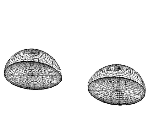
Figure 6: Shape of irrotational binary neutron stars of baryon mass $M_{\rm B}=1.625\,M_{\odot}$, when the coordinate separation between their centers (density maxima) is $41{\rm\ km}$. Only one half of each star is represented (the part which is above the orbital plane). The drawing is that of the numerical grid, which coincides with the surface of the star, thanks to the use of surface-fitted spherical coordinates.

The velocity field with respect to the co-orbiting observer, as defined by Eq. (52) of Ref. [15], is shown in Fig. 7. Note that this field is tangent to the surface of the star, as it must be.

The lapse function $N$ (cf. Eq. 2) is represented in Fig. 8. The coordinate system $(x,y,z)$ is centered on the intersection between the rotation axis and the orbital plane. The $x$ axis joins the two stellar centers, and the orbital is the $z=0$ plane. The value of $N$ at the center of each star is $N_{\rm c}=0.64$.

The conformal factor $A^{2}$ of the 3-metric [cf. Eq. (2)] is represented in Fig. 9. Its value at the center of each star is $A^{2}_{\rm c}=2.20$.

The shift vector of nonrotating coordinates, $\bf N$, (defined by Eq. (9) of Ref. [14]) is shown in Fig. 10. Its maximum value is $0.10\,c$.

The $K_{xy}$ component of the extrinsic curvature tensor of the hypersurfaces $t={\rm const}$ is shown in Fig. 11. We chose to represent the $K_{xy}$ component because it is the only component of $K_{ij}$ for which none of the sections in the three planes $x=0$, $y=0$ and $z=0$ vanishes.

Figure 7: Velocity field with respect to the co-orbiting observer, for the configuration shown in Fig. 6. The plane of the figure is the orbital plane. The heavy line denotes the surface of the star. The companion is located at $x=+41{\rm\ km}$.

Figure 8: Isocontour of the lapse function $N$ for the configuration shown in Fig. 6. The plots are cross section is the $x=0$, $y=0$ and $z=0$ planes (note that the $x$ coordinate is shifted by $20.5{\rm\ km}$ with respect to that of Fig. 7). The dot-dashed line denotes the boundary between the inner numerical grid and the outer compactified one (which extends to spatial infinity), for the grid system centered on the intersection between the rotation axis and the orbital plane.

Figure 9: Same as Fig. 8 but for the conformal factor $A^{2}$ of the spatial metric.

Figure 10: Shift vector of nonrotating coordinates in the orbital plane, for the configuration shown in Figs. 6-9.

Figure 11: Same as Fig. 8 but for the component $K_{xy}$ of the extrinsic curvature tensor. The solid (resp. dashed) lines corresponds to positive (resp. negative) values of $K_{xy}$.

The variation of the central density along the $M_{\rm B}=1.625\,M_{\odot}$ sequence is shown in Fig. 12. We have also computed a corotating sequence for comparison (dashed line in Fig. 12). In the corotating case, the central density decreases quite substantially as the two stars approach each other. This is in agreement with the results of Baumgarte et al. [7, 8]. In the irrotational case (solid line in Fig. 12), the central density remains rather constant (with a slight increase, below $0.1\%$) before decreasing. We can thus conclude that no tendency to individual gravitational collapse is found in this case. This contrasts with results of dynamical calculations by Mathews et al. [12] which show a central density increase of $14\%$ for the same compactification ratio $M/R=0.14$.

Figure 12: Relative variation of the central energy density $e_{\rm c}$ with respect to its value at infinite separation $e_{\rm c}^{\rm inf}$ as a function of the coordinate separation $d$ (or of the orbital frequency $\Omega/(2\pi)$) for constant baryon mass $M_{\rm B}=1.625\,M_{\odot}$ sequences. The solid (resp. dashed) line corresponds to a irrotational (resp. corotating) sequence of coalescing neutron star binaries (Figure from Ref. [14]).

4.3 Irrotational sequence with $M/R=0.17$

In order to investigate how the above result depends on the compactness of the stars, we have computed an irrotational sequence with a baryon mass $M_{\rm B}=1.85\,M_{\odot}$, which corresponds to a compactification ratio $M/R=0.17$ for stars at infinite separation (second heavy dot in Fig. 5). The result is compared with that of $M/R=0.14$ in Fig. 13. A very small density increase (at most $0.3\%$) is observed before the decrease. Note that this density increase remains within the expected error ($\sim 2\%$, cf. Sect. 2.1) induced by the conformally flat approximation for the 3-metric, so that it cannot be asserted that this effect would remain in a complete calculation.

Marronetti, Mathews and Wilson [31] have recently computed quasiequilibrium irrotational configurations by means of a new code. They use a higher compactification ratio, $M/R=0.19$ (third heavy dot in Fig. 5). They found a central density increase as the orbit shrinks much pronounced than that we found for the compactification ratio $M/R=0.17$: $3.5\%$ against $0.3\%$. We will present irrotational sequences with the compactification ratio $M/R=0.19$ and compare with the results by Marronetti et al. [31] in a future article.

Figure 13: Relative variation of the central energy density $e_{\rm c}$ with respect to its value at infinite separation $e_{\rm c}^{\rm inf}$ as a function of the coordinate separation $d$ for constant baryon mass sequences with $M_{\rm B}=1.625\,M_{\odot}$ (solid line, same as in Fig. 12) and $M_{\rm B}=1.85\,M_{\odot}$ (dashed line).

5 Innermost stable circular orbit

An important parameter for the detection of a gravitational wave signal from coalescing binaries is the location of the innermost stable circular orbit (ISCO), if any. In Table 2, we recall what is known about the existence of an ISCO for extended fluid bodies. The case of two point masses is discussed in details in Ref. [2].

Model	Existence of an ISCO	References
Newtonian corotating	ISCO $\Leftrightarrow\,\gamma>2$	[32]
Newtonian irrotational	ISCO $\Leftrightarrow\,\gamma>2.4$	[29]
GR corotating	ISCO $\Leftrightarrow\,\gamma>5/3$	[7], [32]
GR irrotational	ISCO exists for $\gamma=\infty$	[3]

Table 2: Known results about the existence of an ISCO for extended fluid bodies, in terms of the adiabatic index $\gamma$.

For Newtonian binaries, it has been shown [33] that the ISCO is located at a minimum of the total energy, as well as total angular momentum, along a sequence at constant baryon number and constant circulation (irrotational sequences are such sequences). The instability found in this way is dynamical. For corotating sequences, it is secular instead [33, 34]. This turning point method also holds for locating ISCO in relativistic corotating binaries [35]. For relativistic irrotational configurations, no rigorous theorem has been proven yet about the localization of the ISCO by a turning point method. All what can be said is that no turning point is present in the irrotational sequences considered in Sect. 4: Fig. 14 shows the variation as the orbit shrinks of the ADM mass of the spatial hypersurface $t={\rm const}$ (which is a measure of the total energy, or equivalently of the binding energy, of the system) for the $M_{\rm B}=1.625\,M_{\odot}$ sequence. Clearly, the ADM mass decreases monoticaly, without showing any turning point. Figure 15 shows the evolution of the total angular momentum along the same sequence. Again there is no turning point. The same behaviour holds for the $M_{\rm B}=1.85\,M_{\odot}$ sequence, as shown in Figs. 16 and 17.

Figure 14: Half of the ADM mass of the binary system as a function of the coordinate distance $d$, along the evolutionnary sequence $M_{\rm B}=1.625\,M_{\odot}$.

Figure 15: Total angular momentum of the binary system as a function of the coordinate distance $d$, along the evolutionary sequence $M_{\rm B}=1.625\,M_{\odot}$.

Figure 16: Half of the ADM mass of the binary system as a function of the coordinate distance $d$, along the evolutionary sequence $M_{\rm B}=1.85\,M_{\odot}$.

Figure 17: Total angular momentum of the binary system as a function of the coordinate distance $d$, along the evolutionary sequence $M_{\rm B}=1.85\,M_{\odot}$.

6 Conclusion and perspectives

We have computed evolutionary sequences of quasiequilibrium irrotational configurations of binary stars in general relativity. The evolution of the central density of each star have been monitored as the orbit shrinks. For a compactification ratio $M/R=0.14$, the central density remains rather constant (with a slight increase, below $0.1\%$) before decreasing. For a higher compactification ratio $M/R=0.17$ (i.e. stars closer to the maximum mass configuration), a very small density increase (at most $0.3\%$) is observed before the density decrease. It can be thus concluded that no substantial compression of the stars is found, which means that no tendency to individually collapse to black hole prior to merger is observed. Moreover, the observed density increase remains within the expected error ($\sim 2\%$, cf. Sect. 2.1) induced by the conformally flat approximation for the 3-metric, so that it cannot be asserted that this effect would remain in a complete calculation.

No turning point has been found in the binding energy or angular momentum along evolutionary sequences, which may indicate that these systems do not have any innermost stable circular orbit (ISCO).

All these results have been obtained for a polytropic EOS with the adiabatic index $\gamma=2$. We plan to extend them to other values of $\gamma$ in the near future. We also plan to abandon the conformally flat approximation for the 3-metric and use the full Einstein equations, keeping the helicoidal symmetry in a first stage.

References

References

- [1] L. Blanchet, B.R. Iyer, in N. Dadhich and J. Narlikar, editors, Gravitation and relativity: at the turn of the millennium (Inter-University Centre for Astronomy and Astrophysics, Pune, 1998), page 403.
- [2] A. Buonanno, T. Damour, Phys. Rev. D 59, 084006 (1999).
- [3] K. Taniguchi, Prog. Theor. Phys. 101, in press (preprint: gr-qc/9901048).
- [4] K. Oohara and T. Nakamura, in J.A. Marck and J.P. Lasota, editors, Relativistic Gravitation and Gravitational Radiation (Cambridge University Press, Cambridge, England, 1997), page 309.
- [5] J.R. Wilson and G.J. Mathews, Phys. Rev. Lett. 75, 4161 (1995).
- [6] J.R. Wilson, G.J. Mathews, and P. Marronetti, Phys. Rev. D 54, 1317 (1996).
- [7] T.W. Baumgarte, G.B. Cook, M.A. Scheel, S.L. Shapiro, and S.A. Teukolsky, Phys. Rev. Lett. 79, 1182 (1997).
- [8] T.W. Baumgarte, G.B. Cook, M.A. Scheel, S.L. Shapiro, and S.A. Teukolsky, Phys. Rev. D 57, 7299 (1998).
- [9] P. Marronetti, G.J. Mathews, and J.R. Wilson, Phys. Rev. D 58, 107503 (1998).
- [10] C.S. Kochanek, Astrophys. J. 398, 234 (1992).
- [11] L. Bildsten and C. Cutler, Astrophys. J. 400, 175 (1992).
- [12] G.J. Mathews, P. Marronetti, and J.R. Wilson, Phys. Rev. D 58, 043003 (1998).
- [13] E.E. Flanagan, Phys. Rev. Lett. 82, 1354 (1999).
- [14] S. Bonazzola, E. Gourgoulhon, and J-A. Marck, Phys. Rev. Lett. 82, 892 (1999).
- [15] S. Bonazzola, E. Gourgoulhon, and J-A. Marck, Phys. Rev. D 56, 7740 (1997).
- [16] S Bonazzola, E. Gourgoulhon, P. Haensel, and J-A. Marck, in R.A. d’Inverno, editor, Approaches to Numerical Relativity (Cambridge University Press, Cambridge, England, 1992), page 230.
- [17] H. Asada, Phys. Rev. D 57, 7292 (1998).
- [18] S.A. Teukolsky, Astrophys. J. 504, 442 (1998).
- [19] M. Shibata, Phys. Rev. D 58, 024012 (1998).
- [20] L.D. Landau and E.M. Lifchitz, Mécanique des fluides (Mir, Moscow, 1989).
- [21] J.R. Wilson and G.J. Mathews, in C.R. Evans, L.S. Finn, and D.W. Hobill, editors, Frontiers in numerical relativity (Cambridge University Press, Cambridge, England, 1989), page 306.
- [22] G.B. Cook, S.L. Shapiro, and S.A. Teukolsky, Phys. Rev. D 53, 5533 (1996).
- [23] L. Blanchet, G. Faye, B. Ponsot, Phys. Rev. D 58, 124002 (1998).
- [24] R.H. Boyer, Proc. Cambridge Phil. Soc. 61, 527 (1965).
- [25] B. Carter, in C. Hazard and S. Mitton, editors, Active Galactic Nuclei (Cambridge University Press, Cambridge, England, 1979), page 273.
- [26] S. Bonazzola, E. Gourgoulhon, and J-A. Marck, Phys. Rev. D 58, 104020 (1998).
- [27] S. Bonazzola, E. Gourgoulhon, and J-A. Marck, J. Comp. Appl. Math., in press (preprint: gr-qc/9811089).
- [28] J-A. Marck and E. Gourgoulhon, Langage Objet pour la RElativité NumériquE – library documentation, in preparation.
- [29] K. Uryu and Y. Eriguchi, Mon. Not. Roy. Astron. Soc. 296, L1 (1998).
- [30] K. Uryu and Y. Eriguchi, Astrophys. J. Suppl. 118, 563 (1998).
- [31] P. Marronetti, G.J. Mathews, and J.R. Wilson, this volume (preprint: gr-qc/9903105).
- [32] M. Shibata, K. Taniguchi, T. Nakamura, Prog. Theor. Phys. Suppl. 128, 295 (1997).
- [33] D. Lai, F.A. Rasio, S.L. Shapiro, Astrophys. J. Suppl. 88, 205 (1993).
- [34] D. Lai, F.A. Rasio, S.L. Shapiro, Astrophys. J. 423, 344 (1994).
- [35] T.W. Baumgarte, G.B. Cook, M.A. Scheel, S.L. Shapiro, and S.A. Teukolsky, Phys. Rev. D 57, 6181 (1998).