Renormalized stress tensor in one-bubble spacetimes

Abstract

We compute the two-point function and the renormalized expectation value of the stress tensor of a quantum field interacting with a nucleating bubble. Two simple models are considered. One is the massless field in the Vilenkin-Ipser-Sikivie spacetime describing the gravitational field of a reflection symmetric domain wall. The other is vacuum decay in flat spacetime where the quantum field only interacts with the tunneling field on the bubble wall. In both cases the stress tensor is of the perfect fluid form. The assymptotic form of the equation of state are given for each model. In the VIS case, we find that $p=-(1/3)\rho$, where the energy density $\rho$ is dominated by the gradients of supercurvature modes.

1 Introduction

The problem of the quantum state of a nucleating bubble has been addressed in the literature several times[1, 2, 3, 4, 5]. The results relevant for our discussion can be summarized as follows. We have a self-interacting scalar field $\sigma$ (the tunneling field) described by the lagrangian

$${\mathcal{L}}_{\sigma}=-\frac{1}{2}\partial_{\mu}\sigma\partial^{\mu}\sigma-V(\sigma)$$ (1)

where $V(\sigma)$ has a local (metastable) minimum at some value $\sigma_{F}$ and a global one at $\sigma_{T}$ (see Fig. 1). The bubble nucleation can be pictured as the evolution of the $\sigma$ field in imaginary time. The solution of the corresponding Euclidean time equation which interpolates between the false vacuum at spacetime infinity and the true vacuum inside the bubble is called the bounce. In the absence of gravity, vacuum decay is dominated by the $O(4)$ symmetric bounce solution [6]. So we shall write the tunneling field as a function of $\tau\equiv(T_{E}^{2}+{\bf X})^{1/2}$ alone,

$$\sigma=\sigma_{0}(\tau),$$ (2)

where $(T_{E},{\bf X})$ are Cartesian coordinates in Euclidean space. The solution describing the bubble after nucleation is given by the analytic continuation of the bounce to Minkowski time $T$ through the substitution $T_{E}=-iT$. Then, the bubble solution depends only on the Lorentz invariant quantity $({\bf X}^{2}-T^{2})^{1/2}$, where $(T,{\bf X})$ are the usual Minkowski coordinates.

If there are quantum fields interacting with the tunneling field, their state will be significantly affected by the change of vacuum state. Pioneering investigations of this matter were carried out by Rubakov [2] and Vachaspati and Vilenkin [3]. These latter authors considered a model of two interacting scalar fields $\sigma$ and $\Phi$, and found the quantum state for $\widehat{\bf\Phi}$ (the quantum counterpart of $\Phi$) by solving its functional Scrödinger equation. In order to find a solution, they impose as boundary conditions for the wave function $\Psi(\tau;\Phi]$ regularity under the barrier and the tunneling boundary condition (see [3] for details). They found that the quantum state must be SO(3,1) invariant.

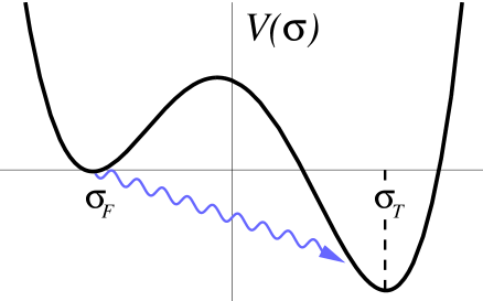
Figure 1: Assumed shape for the potential of the tunneling field. It has a local minimum which corresponds to the false vacuum at $\sigma_{F}$ and a global minimum, the true vacuum, at $\sigma_{T}$. The bounce corresponds to the Euclidean evolution of the tunneling field under the barrier.

A somewhat different approach was pursued later by Sasaki and Tanaka [4]. They carried out a refinement of the method for constructing the WKB wave function for multidimensional systems, first introduced by Banks, Bender and Wu [7] and extended to field theory by Vega, Gervais and Sakita [8], and obtained the so called quasi-ground state wave function. The quasi-ground state wave function is a solution of the time independent functional Schrödinger equation to the second order in the WKB approximation which is sufficiently localized at the false vacuum so that it would be the ground state wave functional it there were no tunneling. They also found that the state must be SO(3,1) invariant.

Moreover, general arguments, due to Coleman [9], suggest that the decay must be SO(3,1) invariant. If not, the infinite volume Lorentz group will make the nucleation probability diverge. From a practical point of view, therefore, it would be interesting to know to what extent symmetry considerations alone can be used to determine the quantum state after nucleations. As a first approach to this question it will be useful to compute the two-point function and the renormalized expectation value of the stress tensor in a SO(3,1) invariant quantum state for two simples models of one-bubble spacetimes.

2 General Formalism

Our aim is to study the quantum state of a field $\Phi$ described by a Lagrangian of the general form

$${\mathcal{L}}_{\Phi}=-\frac{1}{2}\partial_{\mu}\Phi\partial^{\mu}\Phi-\frac{1}{2}m(\sigma)^{2}\Phi^{2},$$ (3)

where the mass term is due to the interaction of the field $\Phi$ with a nucleating bubble. Working from the very beginning in the Heisenberg picture, we will construct an SO(3,1) invariant quantum state for the field $\widehat{\bf\Phi}$. After we will find its Hadamard two-point function $G^{(1)}(x,x^{\prime})\equiv\langle 0|\{\widehat{\bf\Phi},(x)\widehat{\bf\Phi}(x^{\prime})\}|0\rangle$, and we will check whether it is of the Hadamard form [10, 11, 12, 13]. Loosely speaking, a Hadamard state can be described as a state for which the singular part of $G^{(1)}(x,x^{\prime})$ takes the form

$$G^{(1)}_{\rm sing}(x,x^{\prime})=\frac{u}{\sigma}+v\log(\sigma),$$ (4)

where $\sigma$ denotes half of the square of the geodesic distance between $x$ and $x^{\prime}$, and $u$ and $v$ are smooth functions that can be expanded as a power series in $\sigma$, at least for $x^{\prime}$ in a small neighborhood of $x$. Hadamard states are considered physically acceptable because for them the point-splitting prescription gives a satisfactory definition of the expectation value of the stress-energy tensor. After clarifying the singular structure of $G^{(1)}(x,x^{\prime})$, we will use the point-splitting formalism [14, 15, 16, 17] to compute the renormalized expectation value of the energy-momentum tensor in this quantum state. Finally we will briefly discuss the applicability of a uniqueness theorem for quantum states due to Kay and Wald [13].

3 SO(3,1) coordinates

In the present paper we will restrict ourselves to piecewise flat spacetime. It proves very useful to use coordinates adapted to the symmetry of the problem. So we will coordinatize flat Minkowski space using hyperbolic slices, which will embody the symmetry under Lorentz transformations. We define the new coordinates $(t,r)$ (Milne coordinates) by the equations

$$t\equiv(T^{2}-{\bf X}^{2})^{1/2}\hskip 28.45274ptr\equiv\mbox{tanh}^{-1}(|{\bf X}|/T),$$ (5)

where $(T,{\bf X})$ are the usual Minkowski coordinates. In terms of these coordinates, we have

$$ds^{2}=-dt^{2}+t^{2}d\Omega_{H_{3}},$$ (6)

where

$$d\Omega_{H_{3}}=dr^{2}+\sinh^{2}r\,d\Omega_{S_{2}}$$ (7)

is the metric on the unit 3-dimensional spacelike hyperboloid, and $d\Omega_{S_{2}}$ is the line element on a unit sphere.

The above coordinates cover only the interior of the lightcone from the origin. In order to cover the exterior, we will use the Rindler coordinates

$$\xi_{R}\equiv({\bf X}-T^{2})^{1/2}\hskip 28.45274pt\chi_{R}\equiv\mbox{tanh}^{-1}(T/|{\bf X}|).$$ (8)

In terms of this coordinates, the line element reads

$$ds^{2}=d\xi_{R}^{2}+g_{AB}dx^{A}dx^{B}=d\xi_{R}^{2}+\xi_{R}^{2}\,d\Omega_{dS_{3}},$$ (9)

where $g_{AB}$ is the metric on the $\xi_{R}=\mbox{ct.}$ hypersurfaces, and $dS_{3}$ is the line element on a unit “radius” (2+1)-dimensional de Sitter space,

$$d\Omega_{dS_{3}}=-d\chi_{R}^{2}+\cosh^{2}\chi_{R}\,d\Omega_{S_{2}}.$$ (10)

The Milne and the Rindler coordinates are related by analytic continuation,

$$\chi_{R}=r-i\pi/2\hskip 28.45274pt\xi_{R}=it.$$ (11)

Notice that $t$ is timelike inside the lightcone and becomes spacelike after analytical continuation to the outside, whereas $r$ is spacelike inside the lightcone but its analytical continuation is time-like.

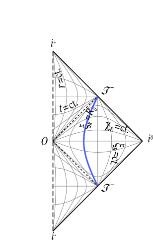
Figure 2: Conformal diagram of Minkowski spacetime. The Milne coordinates $(t,r)$ cover the region inside the lightcone emanating from the origin $O$. The Rindler coordinates $(\xi_{R},\chi_{R})$ cover the outside of this lightcone. The thicker solid line in the central diamond shaped region corresponds to the position of the bubble wall.

4 Quantum state

Here we will consider two simple models. First we shall consider a massless field living in the Vilenkin-Ipser-Sikivie spacetime[18]. The VIS spacetime represents the global gravitational field of a reflection symmetric domain wall, and can be constructed by gluing two Minkowski spaces at some $\xi_{R}=R_{0}$, the locus corresponding to the evolution of the bubble wall (see Fig. 3). The second model we will study is a field which interacts with the tunneling field only on the bubble wall. For the tunneling field, we will assume the thin bubble wall approximation. More general models of the form (3) will be considered elsewhere[25].

The quantization will be performed in the “Rindler wedges” of these spaces, because the hypersurfaces $\chi_{R}=\text{ct.}$ are Cauchy surfaces for the whole spacetime.

4.1 VIS model

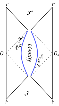
Figure 3: Conformal diagram of the VIS spacetime. This spacetime, which corresponds to the global gravitational field of a reflection symmetric domain wall, is constructed by identifying two Minkowski spacetimes at some $\xi_{R}=R_{0}$.

Here we consider a massless field living in a spacetime constructed by gluing two Minkowski spaces at some $\xi_{R}=R_{0}$. We take Rindler coordinates in the region outside the origin of the two pieces, using a Rindler patch for each one. On each side, the Rindler coordinate ${}^{(l/r)}\xi_{R}$ , where the index $l$ or $r$ refers to the left or right pieces, ranges from ${}^{(l/r)}\xi_{R}=0$ on the lightcone to some value ${}^{(l/r)}\xi_{R}=R_{0}$, where the two Minkowski pieces are identified. Defining ${}^{(l)}\xi_{R}=R_{0}e^{\eta}$ and ${}^{(r)}\xi_{R}=R_{0}e^{-\eta}$, we can coordinatize both pieces letting $\eta$ range from $-\infty$ to $\infty$. Then the line element outside the lightcone becomes

$$ds^{2}=a(\eta)^{2}\left(d\eta^{2}-d\chi_{R}^{2}+\cosh^{2}\chi_{R}d\,\Omega_{2}\right),$$ (12)

where $a(\eta)=R_{0}e^{\eta}\theta(-\eta)+R_{0}e^{-\eta}\theta(\eta)$. Here $\theta(x)$ is the Heaviside step function.

In order to construct a quantum state, we expand the field operator $\widehat{\bf\Phi}$ in terms of a sum over a complete set of mode functions times the corresponding creation and annihilation operators,

$$\widehat{\bf\Phi}=\sum_{plm}a_{plm}\Phi_{plm}+\mbox{h.c.},$$ (13)

The mode functions $\Phi_{plm}$ satisfy the field equation

$$\Box\Phi_{plm}=0,$$ (14)

where $\Box$ stands here for the four dimensional d’Alambertian operator in the VIS spacetime. Taking the ansatz

$$\Phi_{plm}=\frac{F_{p}(\eta)}{a(\eta)}{\mathcal{Y}}_{plm}(\tilde{x})$$ (15)

where $\tilde{x}=(\chi_{R},\Omega)$, $\Omega=(\theta,\varphi)$, equation (14) decouples into

$${}^{dS}\Box{\mathcal{Y}}_{plm} =(p^{2}+1){\mathcal{Y}}_{plm}$$ (16)

$$\left[-\frac{d^{2}}{d\eta^{2}}-2\delta(\eta)\right]F_{p} =p^{2}F_{p}.$$ (17)

Here ${}^{dS}\Box$ stands for the covariant d’Alembertian on a (2+1) de Sitter space. Equations (16)-(17) have the interpretation that ${\mathcal{Y}}_{plm}$ are massive fields living in a (2+1) de Sitter space, with the mass spectrum given by the eigenvalues of the Schrödinger equation for $F_{p}$. Solving (17), we find that the spectrum has a continuous two-fold degenerate part for $p^{2}>0$ and a bound state with $p^{2}=-1$ (a zero mode). If we let $p$ take positive and negative values, the normalized mode functions $F_{p}$ for $p^{2}>0$, which are the usual scattering waves, can be written as

$$F_{p}=\frac{1}{\sqrt{2\pi}}\left((e^{ip\eta}+\rho(p)e^{-ip\eta})\theta(-\mbox{sgn}(p)\,\eta)\ +\sigma(p)e^{ip\eta}\theta\left(\mbox{sgn}(p)\,\eta\right)\right),$$ (18)

where

$$\rho(p) =-\frac{1}{i|p|+1},$$ (19)

$$\sigma(p) =\frac{i|p|}{i|p|+1}.$$ (20)

The normalized supercurvature mode $p^{2}=-1$ is given by

$$F_{,-1}=\frac{a(\eta)}{R_{0}},$$ (21)

where the coma indicates that $-1$ refers to $p^{2}$ instead of $p$. As we are interested in a SO(3,1) invariant state, the natural choice for ${\mathcal{Y}}_{plm}$ are the positive frequency (2+1) Bunch-Davies modes [19],

$${\mathcal{Y}}_{plm}(\tilde{x})=\sqrt{\frac{\Gamma(l+1+ip)\Gamma(l+1-ip)}{2}}\frac{P_{ip-1/2}^{-l-1/2}(i\sinh\chi_{R})}{\sqrt{i\cosh\chi_{R}}}Y_{lm}(\Omega),$$ (22)

where $Y_{lm}(\Omega)$ are the usual spherical harmonics. With this choice, it is straightforward to show that the quantum state for $\widehat{\Phi}$ is SO(3,1) invariant.

Now we proceed to compute the two-point Wightman function $G^{(+)}(x,x^{\prime})$,

$$G^{(+)}(x,x^{\prime}) \equiv\langle 0|\widehat{\bf\Phi}(x)\widehat{\bf\Phi}(x^{\prime})|0\rangle=\sum_{lm}\Phi_{-1,lm}(x)\overline{\Phi_{-1,lm}(x^{\prime})}$$

$$+\int_{-\infty}^{\infty}dp\sum_{lm}\Phi_{plm}(x)\overline{\Phi_{plm}(x^{\prime})}.$$ (23)

From now on we will suppose that the two points $x$ and $x^{\prime}$ belong to the Rindler wedge of the “left Minkowski” space, so we will omit the $(l)$ index for notational simplicity. Direct substitution of the mode functions gives

$$G^{(+)}(x,x^{\prime}) =\frac{1}{R_{0}^{2}}\sum_{lm}{\mathcal{Y}}_{-1,lm}(\tilde{x})\overline{{\mathcal{Y}}_{-1,lm}(\tilde{x}^{\prime})}$$

$$+\frac{1}{2\pi R_{0}^{2}}\int^{\infty}_{-\infty}dp\left(\xi_{M}^{ip-1}\xi^{\prime}_{M}{}^{-ip-1}\right.$$

$$+\left.\frac{1}{ip-1}\xi_{M}^{ip-1}\xi^{\prime}_{M}{}^{ip-1}\right)\sum_{lm}{\mathcal{Y}}_{plm}(\tilde{x})\overline{{\mathcal{Y}}_{plm}(\tilde{x}^{\prime})},$$ (24)

where we have defined $\xi_{M}=e^{\eta}=\xi_{R}/R_{0}$. The two-point function $G^{(+)}$ is SO(3,1) invariant because is a sum of SO(3,1) invariant terms. Due to our choice of positive frequency modes, the $lm$ sums correspond to the two-point Wightman functions in the Euclidean vacuum for massive and a massless scalar fields living in $(2+1)$ de Sitter spacetime. The (3+1)-dimensional Lorentz group SO(3,1) is the same as the group of (2+1)-dimensional de Sitter transformations, so the two-point functions are Lorentz invariant by construction (its explicit form is given below). $G^{(+)}$ also depens on the quantity $\xi_{R}$. This is a function of the interval in Minkowski space time, so it is Lorentz invariant too.

Figure 4: Conformal diagram of a (2+1) de Sitter hyperboloid $\xi_{R}$=ct. Without loss of generality, we can take the point $\tilde{x}$ to lie in the “origin” O. Then $Z>1$ if $\tilde{x}^{\prime}$ is timelike related with the origin, and $-1<Z<1$ if $\tilde{x}^{\prime}$ is spacelike related with the origin and can be joined with it by means of a geodesic. If $Z<-1$, $\tilde{x}^{\prime}$ is spacelike related with the origin but there are no geodesics connecting it with the origin. The function $\epsilon(x,x^{\prime})$ is introduced in order to take into account the time ordering of those points which are timelike related. If this is the case, it evaluates to $\varepsilon$ if $\chi_{R}>\chi_{R}^{\prime}$ and to $-\varepsilon$ if $\chi_{R}<\chi_{R}^{\prime}$, where $\varepsilon$ is a small positive value. Two possible paths for $\chi^{\prime}_{R}$ which pass through the origin are drawn (see discussion in Fig. 5)

First we will compute the contribution of the continuum. The $lm$ sum has been explicitly computed [24],

$$G^{(+)}_{p}(\tilde{x},\tilde{x}^{\prime}) \equiv\sum_{lm}{\mathcal{Y}}_{plm}\overline{{\mathcal{Y}}_{plm}}$$

$$=\frac{\Gamma(1+ip)\Gamma(1-ip)}{(4\pi)^{3/2}\Gamma(3/2)}{}_{2}F_{1}\left[1+ip,1-ip;\frac{3}{2};{\frac{1+Z-i\epsilon}{2}}\right],$$ (25)

where $Z(\tilde{x},\tilde{x}^{\prime})\equiv X^{\mu}(\tilde{x})X_{\mu}(\tilde{x}^{\prime})=-\sinh\chi_{R}\sinh\chi_{R}^{\prime}+\cosh\chi_{R}\cosh\chi_{R}^{\prime}\cos\widehat{\Omega\Omega^{\prime}}$, which is explicitly Lorentz invariant. Here $X^{\mu}(\tilde{x})$ is the position of the point $\tilde{x}$ in the (3+1) Minkowski space where the $(2+1)$ de Sitter space is embedded as a timelike hyperboloid. The function $\epsilon(\tilde{x},\tilde{x}^{\prime})$ has been introduced to indicate at which side of the cut the hypergeometric function should be computed. It evaluates to $\varepsilon$ if $\tilde{x}$ and $\tilde{x}^{\prime}$ are timelike related and $\chi_{R}>\chi_{R}^{\prime}$, to $-\varepsilon$ if $\tilde{x}$ and $\tilde{x}^{\prime}$ are timelike related and $\chi_{R}<\chi_{R}^{\prime}$, and vanishes if $\tilde{x}$ and $\tilde{x}^{\prime}$ are spacelike related, where $\varepsilon$ is a small positive constant (see Fig. 4). At the end of the calculation, we will take the limit $\varepsilon\to 0$. Introducing $\cos\tilde{\zeta}\equiv-\tilde{Z}\equiv-Z+i\epsilon$, the two-point function $G^{(+)}_{p}(\tilde{x},\tilde{x}^{\prime})$ can be compactly written as

$$G^{(+)}_{p}(\tilde{x},\tilde{x}^{\prime})=\frac{1}{4\pi\sin\tilde{\zeta}}\frac{\sinh p\tilde{\zeta}}{\sinh\pi p}.$$ (26)

After performing the $p$ integration we obtain

$$G^{(+)}_{\rm cont}(x,x^{\prime}) =\frac{1}{8\pi^{2}\sigma}+\frac{1}{8\pi R_{0}^{2}}\left(2\cot\tilde{\zeta}\left(\tilde{\zeta}-\mbox{arc tan}\frac{\sin\tilde{\zeta}}{\cos\tilde{\zeta}+\xi_{M}\xi_{M}^{\prime}}\right)\right.$$

$$+\left.\log\frac{(\xi_{M}\xi^{\prime}_{M})^{2}}{\sin\tilde{\zeta}^{2}+(\cos\tilde{\zeta}+\xi_{M}\xi^{\prime}_{M})^{2}}\right).$$ (27)

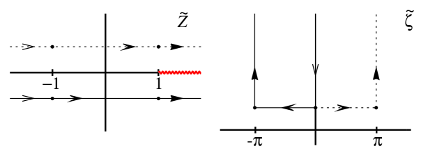
Figure 5: Paths in the complex $\tilde{Z}$- and $\tilde{\zeta}$-planes for the curves shown in Fig. 4, where we hold the point $\tilde{x}$ fixed at O while moving $\tilde{x}^{\prime}$ around the $(2+1)$ de Sitter space. If $Z<-1$, then $\tilde{\zeta}$ is purely imaginary. If $-1<Z<1$, $\tilde{\zeta}$ is essentially real (if it were not for the small $i\epsilon$ imaginary part). In this case, if $\chi_{R}<\chi_{R}^{\prime}$, $-\pi<\tilde{\zeta}<0$, but if $\chi_{R}>\chi_{R}^{\prime}$ then $0<\tilde{\zeta}<\pi$. The coincidence limit corresponds to both $\tilde{\zeta}=\pm\pi$, depending on that we approach $\tilde{x}$ from “abov” or “below”. When $\tilde{x}$ and $\tilde{x}^{\prime}$ are timelike related, $\tilde{\zeta}$ has both imaginary and real parts. Its real part is $\pm\pi$ depending on whether $\chi_{R}$ is greater or less than $\chi_{R}^{\prime}$, respectively.

The “supercurvature” contribution of the $p^{2}=-1$ mode is in fact divergent. This is related to the zero mode problem of massless quantum fields in spacetimes with compact Cauchy surfaces. Following the usual prescription [20, 21, 22, 23], we formally write this divergent term as a divergent piece plus a finite one,

$$G^{(+)}_{\rm sup}(x,x^{\prime})=\frac{1}{4\pi^{2}}\langle 0|Q^{2}|0\rangle+\sum_{l>0,m}\frac{1}{R_{0}^{2}}{\mathcal{Y}}_{-1,lm}\overline{{\mathcal{Y}}_{-1,lm}},$$ (28)

where the infinity has been hidden in an infinite constant (see [23] for details). After, when taking derivatives to compute the energy-momentum tensor, this divergent constant term will give no contribution. The sum can be performed, and the result is

$$G^{(+)}_{\rm sup}(x,x^{\prime}) =\frac{1}{4\pi^{2}}\langle 0|Q^{2}|0\rangle+\frac{1}{8\pi^{2}R_{0}^{2}}\left(-2\tilde{\zeta}\cot\tilde{\zeta}\right.$$

$$+\left.(2\chi+i\pi)\tanh\chi_{R}+(2\chi^{\prime}-i\pi)\tanh\chi^{\prime}_{R}\frac{}{}\right),$$ (29)

where we have dropped an irrelevant constant.

Adding the continuum and supercurvature contributions, and symmetrizing the result with respect to $x$ and $x^{\prime}$, we finally find the symmetric Hadamard two-point function (for pairs of points $x$, $x^{\prime}$ outside the lightcone in the “left” Minkowski patch),

$$G^{(1)}(x,x^{\prime}) =\frac{1}{4\pi^{2}\sigma}+\frac{1}{4\pi^{2}R_{0}^{2}}\left(2\chi_{R}\tanh\chi_{R}+2\chi^{\prime}_{R}\tanh\chi^{\prime}_{R}\right.$$

$$-\left.2\,\cot\tilde{\zeta}\,\mbox{arc tan}\frac{\sin\tilde{\zeta}}{\cos\tilde{\zeta}+\xi_{M}\xi_{M}^{\prime}}\right.$$

$$+\left.\log\frac{(\xi_{M}\xi^{\prime}_{M})^{2}}{\sin^{2}\tilde{\zeta}+(\cos\tilde{\zeta}+\xi_{M}\xi^{\prime}_{M})^{2}}\right)+\frac{1}{2\pi^{2}}\langle 0|Q^{2}|0\rangle$$

$$=\frac{1}{4\pi^{2}\sigma}+W(x,x^{\prime}),$$ (30)

where

$$\sigma=\frac{1}{2}\left(\xi_{R}^{2}+\xi^{\prime}_{R}{}^{2}+2\xi_{R}\xi^{\prime}_{R}\cos\tilde{\zeta}\right)$$ (31)

is one half of the square geodesic distance in flat spacetime. The first term in the final expression for $G^{(1)}(x,x^{\prime})$ is the usual Minkowski ultraviolet divergence. The second term, $W(x,x^{\prime})$, is due to the nontrivial geometric boundary conditions imposed by the symmetry of our problem. If $W(x,x^{\prime})$ were not singular, the state would be of the Hadamard form[10, 11, 12]. But $W(x,x^{\prime})$ has local and nonlocal singularities. In the coincidence limit, it is divergent on the bubble wall. It is logarithmically singular whenever one of the points is on the lightcone emanating from the origin. It is also singular when $x$ and $x^{\prime}$ satisfy the relation $\sin^{2}\tilde{\zeta}+(\cos\tilde{\zeta}+\xi_{M}\xi^{\prime}_{M})^{2}=0$, so the argument of the logarithm diverges. The roots of this equation are at

$$\xi_{M}^{\rm s}{\xi^{\prime}}^{\rm s}_{M}=-e^{\pm i\tilde{\zeta}_{\rm s}}.$$ (32)

To clarify the position of the singularities, let us fix the point $x_{\rm s}$ and look for the points $x^{\prime}_{\rm s}$ which make $G^{(+)}(x_{\rm s},x^{\prime}_{\rm s})$ singular. Taking into account that $\xi_{M}^{\rm s}$ and ${\xi^{\prime}}^{\rm s}_{M}$ should be real and should satisfy $0<\xi_{M}^{\rm s},{\xi^{\prime}}^{\rm s}_{M}<1$, it is seen from (32) that the allowed values of $\tilde{\zeta}_{\rm s}$ are of the form $\pm\pi+iy$ (i.e., $\tilde{x}_{\rm s}$ and $\tilde{x}^{\prime}_{\rm s}$ are “timelike” separated on a (2+1) de Sitter hyperboloid, see Fig. 5), with $y>-\log\xi_{M}^{\rm s}>0$. Without loss of generality, we can assume that $\tilde{x}_{\rm s}=(0,0,0)$. Then $\cos\tilde{\zeta}_{\rm s}=-\cosh y=-\cosh{\chi_{R}^{\prime}}^{\rm s}\cos\theta^{\prime}_{\rm s}$. This implies that $0\leq\theta^{\prime}_{\rm s}\leq\pi/2$, and we have no restriction on $\varphi^{\prime}_{\rm s}$. Since $\cosh{\chi_{R}^{\prime}}^{\rm s}=\cosh y/\cos\theta^{\prime}_{\rm s}\geq\cosh y$, we find that ${\chi_{R}^{\prime}}^{\rm s}\geq y\geq-\log\xi_{M}^{\rm s}$ or ${\chi_{R}^{\prime}}^{\rm s}\leq-y\leq\log\xi_{M}^{\rm s}$. So the region inside of which (for any value of $\Omega^{\prime}$) $G^{(+)}(x,x^{\prime})$ is non singular (apart from the singular points on the lightcone from $x$) is limited by the curves

Figure 6: Nonlocal singularities in the upper half “left Minkowski”, in the VIS model. Inside the shadowed region the two-point function $G^{(1)}(x,x^{\prime})$, considered as a function of $x^{\prime}$ with $x$ fixed, is singular only on the lightcone from $x$.

$${\xi^{\prime}}^{\rm n.s.}_{M} =\frac{1}{e^{y}\xi_{M}^{\rm s.}}$$ (33)

$${\chi^{\prime}}^{\rm n.s.}_{R} =\pm y,$$ (34)

with $y>-\log\xi_{M}^{\rm s}$, the lightcone from the origin and the bubble wall (the superscript n.s. stands for “nearest (nonlocal) singularity”, see Fig. 6). Note that as $x$ approaches to the bubble wall (i.e., $\xi_{M}\to 1$), the distance to the nearest singular point $x^{\prime}$ reduces. Consistently, in the limiting case when $x$ is on the wall, $W(x,x^{\prime})$ is singular on the coincidence limit.

Let us now check the causal relationship between singular points satisfying equation (32). If we compute $\sigma(x_{\rm s},x^{\prime}_{\rm s})$, we will find

$$\sigma(x_{\rm s},x^{\prime}_{\rm s})=\frac{e^{-2y}}{2\xi_{M}^{{\rm s}\,2}}(1-\xi_{M}^{{\rm s}\,2})(1-\xi_{M}^{{\rm s}\,2}e^{2y})\leq 0,$$ (35)

where the last inequality follows from $y\geq-\log\xi_{M}^{\rm s}$, $0\leq\xi_{M}^{\rm s}\leq 1$. The equality can only be realized if $x_{\rm s}$ is on the bubble wall. Then, in this case, there exist nonlocal singularities (of $W(x,x^{\prime})$) which are null related. But if $x_{\rm s}$ is not on the bubble wall, its singular partners are always time-like related with it.

Summarizing, the two-point function is locally Hadamard everywhere except on the bubble wall and on the lightcone. Moreover, it has (harmless, see discussion below) nonlocal singularities.

4.2 ST model

In this second model, which has previously been considered by Sasaki and Tanaka [5], the $\widehat{\Phi}$ field interacts with the tunneling field $\sigma$ only on the bubble wall. We assume the infinitely thin-wall approximation, so the interaction term can be written as

$$m^{2}(\eta)=2\frac{V_{0}}{R_{0}^{2}}\delta(\eta),$$ (36)

where $V_{0}>0$ characterizes the strength of the interaction and $R_{0}$ is the radius of the bubble wall.

Decomposing the field $\widehat{\bf\Phi}$ as before, we find that the Schrödinger equation for $F_{p}$ takes the form

$$-F^{\prime\prime}_{p}+2V_{0}\delta(\eta)F_{p}=p^{2}F_{p},$$ (37)

Now the spectrum is purely continuous with $p^{2}>0$. The solution of this Schrödinger equation is the scattering basis (18) with the transmission and reflection coefficients given by

$$\rho(p) =\frac{V_{0}}{i|p|-V_{0}},$$ (38)

$$\sigma(p) =\frac{i|p|}{i|p|-V_{0}}.$$ (39)

Following a similar path, we arrive at the following Hadamard two-point function (for points $x$, $x^{\prime}$ in the Rindler wedge and inside the bubble),

$$G^{(1)}(x,x^{\prime}) =\frac{1}{4\pi^{2}\sigma}+\frac{1}{4\pi^{2}i}\frac{1}{\xi_{R}\xi^{\prime}_{R}\sin\tilde{\zeta}}\left({}_{2}F_{1}\left[1,V_{0};V_{0}+1;-e^{i\tilde{\zeta}}\frac{\xi_{R}\xi^{\prime}_{R}}{R_{0}^{2}}\right]\right.$$

$$-\left.{}_{2}F_{1}\left[1,V_{0};V_{0}+1;-e^{-i\tilde{\zeta}}\frac{\xi_{R}\xi^{\prime}_{R}}{R_{0}^{2}}\right]\right)=\frac{1}{4\pi^{2}\sigma}+W(x,x^{\prime}),$$ (40)

which is explicitly SO(3,1) invariant. If we take the coincidence limit, the function $W(x,x^{\prime})$ has divergences on the bubble wall, so the state is not locally Hadamard. Apart from this, it has nonlocal logarithmic singularities at the points where the argument of the hypergeometric functions become 1, i.e., whenever $\xi_{M}\xi_{M}^{\prime}=-\exp(\pm i\tilde{\zeta})$. This is the same relation we found in the VIS model. Borrowing the conclusions from the VIS model, the state is locally Hadamard everywhere except on the bubble wall, and has (harmless) timelike nonlocal singularities (except also on the bubble wall).

As we have seen, the two models we have considered share two singular behaviors: the existence of nonlocal singularities and the singularity of $W(x,x^{\prime})$ in the coincidence limit on the bubble wall. These singularities seem to be related with the oversimplification of the model. Presumably, if instead of a $\delta$-like term interaction we had introduced a smooth function, these divergences would disappear.

5 Renormalized expectation value of the stress tensor

As we have pointed out, for the two models we have studied the singularities of $G^{(1)}(x,x^{\prime})$ are nearly of the Hadamard type. We can use the point-splitting regularization prescription to compute the renormalized expectation value of the stress-energy momentum tensor [14, 15, 16],

$$\langle T_{ab}\rangle =\frac{1}{2}\lim_{x\to x^{\prime}}{\mathcal{D}}_{ab^{\prime}}[W(x,x^{\prime})],$$ (41)

$${\mathcal{D}}_{ab^{\prime}} =\nabla_{a}\nabla_{b^{\prime}}-\frac{1}{2}g_{ab^{\prime}}g^{cd^{\prime}}\nabla_{c}\nabla_{d^{\prime}}.$$ (42)

Noticing that $\cos\tilde{\zeta}=-Z+i\epsilon=-\cos\sqrt{2\,\,^{dS}\sigma}+i\epsilon$, where ${}^{dS}\sigma$ is one half of the square distance in a unit (2+1) de Sitter spacetime, the covariant derivatives in the “de Sitter” direction are easily computed from [14, 12]

$$[^{dS}\sigma_{;A}] =0,$$ (43)

$${[^{dS}\sigma_{;AB^{\prime}}]} =-\frac{g_{AB}}{\xi_{R}^{2}},$$ (44)

where the brackets stand for the coincidence limit.

5.1 VIS model

The renormalized expectation value of the stress tensor turns out to be

$$\langle T_{\xi_{R}\xi_{R}}\rangle =\frac{\xi_{R}^{2}-2R_{0}^{2}}{4\pi^{2}R_{0}^{2}(R_{0}^{2}-\xi_{R}^{2})^{2}},$$ (45)

$$\langle T_{AB}\rangle =-\frac{\xi_{R}^{4}-3R_{0}^{2}\xi_{R}^{2}+6R_{0}^{4}}{12\pi^{2}R_{0}^{2}(R_{0}^{2}-\xi_{R}^{2})^{3}}\,g_{AB}.$$ (46)

where $0\leq\xi_{R}\leq R_{0}$ (i.e., $x$ is in the left Rindler wedge and inside the bubble). It is clear from the expression that the energy-momentum tensor behaves somewhat better than the two-point function. It is divergent on the bubble wall, but behaves smoothly on the lightcone. So it can be analytically continued to the inside of the lightcone. There it behaves like the energy-momentum tensor of a perfect fluid,

$$\langle T_{ab}\rangle=(\rho+p)u_{a}u_{b}+pg_{ab},$$ (47)

where $u^{a}=(\partial_{t})^{a}$. On the lightcone it satisfies the equation of state $p=-\rho$ whith

$$\rho=\frac{1}{2\pi R_{0}^{4}}$$ (48)

For large $t$ the equation of state turns out to be

$$p=-\frac{1}{3}\rho,$$ (49)

with

$$\rho=\frac{1}{4\pi^{2}}\frac{1}{R_{0}^{2}t^{2}}.$$ (50)

Taking into account that the field is massless except on the bubble-wall, one might naively expect that the energy momentum tensor would behave like radiation, with $\rho\propto t^{-4}$. Instead of this, we have found that it decreases slower. In fact, it can be shown that its behaviour is dominated by gradients of the supercurvature modes.

5.2 ST model

For the ST model, we find

$$\langle T_{\xi_{R}\xi_{R}}\rangle =\frac{1}{2\pi^{2}R_{0}^{4}}\frac{V_{0}}{V_{0}+2}{}_{2}F_{1}\left[3,V_{0}+2;V_{0}+3;\left(\frac{\xi_{R}}{R_{0}}\right)^{2}\right],$$ (51)

$$\langle T_{AB}\rangle =\frac{1}{2\pi^{2}R_{0}^{4}}\frac{V_{0}}{V_{0}+2}\left({}_{2}F_{1}\left[3,V_{0}+2;V_{0}+3;\left(\frac{\xi_{R}}{R_{0}}\right)^{2}\right]\right.$$

$$+\left.2\left(\frac{\xi_{R}}{R_{0}}\right)^{2}\frac{V_{0}+2}{V_{0}+3}{}_{2}F_{1}\left[4,V_{0}+3;V_{0}+4;\left(\frac{\xi_{R}}{R_{0}}\right)^{2}\right]\right)g_{AB},$$ (52)

where $0\leq\xi_{R}\leq R_{0}$. As before, the energy-momentum tensor turns out to be singular only on the bubble wall. Continuing analytically the results to the inside of the light-cone, we find that it is of the perfect fluid form. On the lightcone it satisfies the equation of state $p=-\rho$ with

$$\rho=-\frac{1}{2\pi^{2}R_{0}^{4}}\frac{V_{0}}{V_{0}+2}.$$ (53)

For large $t$ the equation of state turns out to be

$$p=\rho,$$ (54)

with

$$\rho=-\frac{4\,R_{0}^{2}}{t^{6}}.$$ (55)

Notice that in this model the energy density is negative and decreases faster than radiation.

6 Discussion

In this paper we have performed the computation of $\langle T_{ab}\rangle$ in a quantum state which fulfills our basic requirement of SO(3,1) invariance. In fact, we have just outlined the most simple method to find a SO(3,1) invariant state. The question is whether by choosing a different set of modes we can also obtain an inequivalent SO(3,1) invariant state but also of the Hadamard form. A theorem due to Kay and Wald [13] is illuminating in this respect. The theorem states that in a spacetime with a bifurcate Killing horizon there can exist at most one regular quasifree state invariant under the isometry which generates the bifurcate Killing horizon. Let us briefly analyze the conditions under which the theorem holds.

In (3+1) spacetimes, we get a bifurcate Killing horizon whenever a one parameter group of isometries leaves invariant a 2-dimensional spacelike manifold $\Sigma$. The bifurcate Killing horizon is generated by the null geodesics orthogonal to $\Sigma$[13]. For example, Minkowski spacetime has bifurcate Killing horizons. The isometry group is a one-parameter subgroup of Lorentz boosts, and the manifold $\Sigma$ is a two-plane. Any SO(3,1) invariant spacetime, where the line element can be written in the form

$$ds^{2}=d\xi_{R}^{2}+a(\xi_{R})^{2}(-d\chi_{R}^{2}+\cosh^{2}\chi_{R}d\Omega),$$ (56)

has a SO(3,1) invariant bifurcate Killing horizon. Noticing that the $\xi_{R}=\mbox{ct.}$ hypersurfaces are (2+1) de Sitter spaces which can be thought as embedded in a (3+1) Minkowski space, any boost generator on these hypersurfaces is the infinitesimal generator of a isometry which 1) leaves invariant a spacelike 2-manifold (so we get a bifurcate Killing horizon) and 2) leaves any SO(3,1) symmetric state invariant. We can take, for example, the boost generator in the $ZT$ plane of the embedding Minkowski space. Expressed in the Rindler coordinates, it becomes

$$\xi^{a}=-\cos\theta\frac{\partial}{\partial\chi_{R}}+\tanh\chi_{R}\sin\theta\frac{\partial}{\partial\theta}.$$ (57)

The Killing field $\xi^{a}$ leaves invariant the spacelike 2-manifold $\theta=\pi/2$, $\chi_{R}=0$. All bubble spacetimes with or without the inclusion of gravity do possess this bifurcate Killing horizon.

A (pure) quasifree ground state is the (wider) algebraic version (see [13] and references therein) of what is usually called a “frequency splitting” Fock vacuum state. A quasifree state has the special property of being completely characterized from its two-point function. A regular quasifree ground state is a quasifree ground state whose two-point symmetric function is globally Hadamard and which has no zero modes. The VIS model has a zero mode (as any massless field in spacetimes with compact Cauchy surfaces have [13]), so the theorem cannot be directly applied. Also strictly speaking, the quantum state we have found for the ST model does not fulfill the requirements of the theorem, because it is not globally Hadamard. Roughly speaking, a two-point function is said to be globally Hadamard if it is locally Hadamard and in addition has nonlocal singularities only at points $x$, $x^{\prime}$ which are null related within a causal normal neighborhood of a Cauchy hypersurface. As we have seen, if we ignore the problems on the bubble wall, the Hadamard function $G^{(1)}(x,x^{\prime}$) we have found for the ST model has nonlocal singularities, but they are timelike related. So, if it were not for the singularities on the bubble wall, the state would be globally Hadamard and without zero modes. As stated before, we think that the singularities on the bubble wall would disappear if the potential were modeled by a smooth function instead of by a $\delta$-like term, making the state globally Hadamard. Then, symmetry would suffice to determine the (physically admissible) quantum state for this model. Generic models which would not present these pathologies will be presented elsewhere[25]

References

- [1] S. Coleman, Phys. Rev. D15, 2929 (1977); C.G. Callan and S. Coleman, ibid. 16, 1762 (1977).
- [2] V.A. Rubakov, Nucl. Phys. B245, 481 (1984).
- [3] T. Vachaspati and A. Vilenkin, Phys. Rev. D43, 3846 (1991).
- [4] T. Tanaka and M. Sasaki, Phys. Rev. D49, 1039 (1994); T. Tanaka and M. Sasaki, ibid. 50, 6444 (1994).
- [5] M. Sasaki, T. Tanaka, K. Yamamoto, and J. Yokoyama, Progr. Theor. Phys. 90, 1019 (1993).
- [6] S. Coleman, V. Glaser and A. Martin, Commun. Math. Phys. 58, 211 (1978).
- [7] T. Banks, C.M. Bender and T. T. Wu, Phys. Rev. D8, 3346(1973); T. Banks and C. M. Bender, ibid. 8, 3366(1973).
- [8] H. J. Vega, J. L. Gervais, and B. Sakita, Nucl. Phys. B139, 20 (1978); ibid. B142, 125 (1978); Phys. Rev. D19, 604 (1979).
- [9] S. Coleman. Aspects of Symmetry. Cambridge University Press, Cambridge, 1985.
- [10] F.G. Friedlander. The Wave Equation on a Curved Spacetime. Cambridge University Press, Cambridge, 1975.
- [11] J. Hadamard. Lectures on Cauchy’s problem in Linear Partial Differential Equations. Yale University Press, New Heaven, CT, 1923.
- [12] B.S. DeWitt. Relativity, Groups and Topology. Gordon and Breach, New York, 1964.
- [13] B. S. Kay and R.M. Wald, Phys. Rep. 207, 49 (1991); B. S. Kay J. Math. Phys. 34, 4519 (1993).
- [14] S. M. Christensen, Phys. Rev. D14, 2490 (1974); S. M. Christensen, Phys. Rev. D17, 946 (1978) .
- [15] R.M. Wald, Commun. Math. Phys. 54, 1 (1977); R.M. Wald, Phys. Rev. D17, 1477 (1978).
- [16] M. R. Brown and A. Ottewill, Phys. Rev. D34, 1776 (1986); D. Bernard and A. Folacci, ibid. 34, 2286 (1986).
- [17] M. Dorca and E. Verdaguer, Nucl. Phys. B484 435 (1997).
- [18] A. Vilenkin Phys. Lett. 133B, 177 (1983); J. Ipser and P. Sikivie, Phys. Rev. D30, 712 (1984).
- [19] T. S. Bunch and P. C. W. Davies, Proc. R. Soc. London A360, 117 (1978).
- [20] B.S. DeWitt. Relativity, Groups and Topology II. North Holland, Amsterdam, 1983.
- [21] L.H. Ford and C. Pathinayake, Phys. Rev. D39, 3642 (1989).
- [22] J. Garriga and A. Vilenkin, Phys. Rev. D45, 3469 (1993).
- [23] K. Kirsten and J. Garriga, Phys. Rev. D48, 567 (1993).
- [24] P. Candelas and D. J. Raine, Phys. Rev. D12, 965 (1975); B. Ratra, Phys. Rev. D31, 1931 (1985) .
- [25] X. Montes, in preparation.