Binary-Induced Collapse Of A Compact, Collisionless Cluster

Abstract

We improve and extend Shapiro’s [1] model of a relativistic, compact object which is stable in isolation but is driven dynamically unstable by the tidal field of a binary companion. Our compact object consists of a dense swarm of test particles moving in randomly-oriented, initially circular, relativistic orbits about a nonrotating black hole. The binary companion is a distant, slowly inspiraling point mass. The tidal field of the companion is treated as a small perturbation on the background Schwarzschild geometry near the hole; the resulting metric is determined by solving the perturbation equations of Regge and Wheeler and Zerilli in the quasi-static limit. The perturbed spacetime supports Bekenstein’s  [13] conjecture that the horizon area of a near-equilibrium black hole is an adiabatic invariant. We follow the evolution of the system and confirm that gravitational collapse can be induced in a compact collisionless cluster by the tidal field of a binary companion.

]

I Introduction

The possibility that massive neutron stars might be driven unstable to collapse to black holes when placed in a close binary orbit was first suggested by Wilson, Mathews and Maronetti (hereafter WMM;  [2]) on the basis of their approximate relativistic numerical simulations. This finding was quite unexpected, partly because it disagreed with earlier Newtonian calculations  [3] which showed that tidal fields stabilize binary stars against radial collapse. In fact, none of the follow-up post-Newtonian (PN) [4]  [5] or approximate analytic analyses  [6] indicate the presence of any relativistic radial instability in fluid binaries, nor does an independent dynamical simulation  [7]. No evidence is found for the WMM “crushing effect” in the relativistic numerical calculations of either corotational  [8] or irrotational  [9] binaries in quasi-equilibrium circular orbits. These later calculations are particularly careful to adopt the same simplifications as WMM (e.g, a conformally flat 3-metric). All of the calculations except those of WMM suggest that the maximum allowed rest mass of a fluid star in a binary is in fact slightly larger than the value in isolation.

While it would appear that the WMM effect may not be present for fluid stars, the work of WMM raises the interesting question as to whether the “crushing instability” might exist for a different type of binary system. Specifically, are there any relativistic binary systems for which tidal fields can trigger the collapse of a compact object known to be stable in isolation? To address this question, Shapiro  [1] offered a simple candidate compact object consisting of a test particle orbiting a Schwarzschild black hole outside the innermost-stable circular orbit (ISCO). Such a “compact object” is obviously stable in isolation, but when it is placed in a binary orbit about a distant mass, an integration of the test-particle equations of motion reveals that the tidal field of the distant mass can cause a test particle to plunge inside the hole.

Shapiro’s model is very promising as a simple illustration of the crushing instability in action, but the original analysis, as he emphasized, was highly simplified and somewhat heuristic. First, the study was confined to two special test-particle orbits, one coplanar with and the other perpendicular to the companion orbital plane. Moreover, the motion of the particle in the perpendicular case was artificially constrained to remain in a plane, precluding any precessional motion or wobbling. Most important, the analysis was based on a post-Newtonian treatment of the 3-body problem in which the tidal piece of the equation for the relative motion of the test particle about the black hole was treated to lowest (Newtonian) order and the nontidal piece replaced by the exact, fully relativistic expression for geodesic motion in Schwarzschild geometry. While such a hybrid approach, similar in spirit to one proposed by Kidder, Will and Wiseman [10] for the 2-body problem, should capture the essential dynamics, it is far from rigorous. In particular, it is not clear a priori how reliable it is to use a Newtonian tidal term when the test particle is moving at high velocity in a very strong gravitational field close to a black hole.

In this paper we improve and extend the simple model presented in  [1] of a compact object subject to binary-induced collapse. We use the equations of Regge and Wheeler  [11] and Zerilli  [12] to derive the perturbation to the spacetime close to a Schwarzschild black hole due to a distant mass. We note in passing that the resulting perturbed spacetime provides another example supporting the recent conjecture of Bekenstein  [13] that the horizon area of a perturbed black hole is an adiabatic invariant. We obtain the geodesic equations of motion in the perturbed spacetime and solve them to track the dynamical evolution of a dense spherical swarm of 20,000 test particles placed around the hole outside the ISCO. The ‘black hole $+$ swarm’ constitutes a compact collisionless cluster whose stability against tidally-induced collapse we determine. We compare our refined treatment with the simpler version presented in  [1] and show that the original equations track the behavior reasonably well. We confirm that the crushing instability can occur in a binary system containing simple compact collisionless clusters like the ones we construct.

II HYBRID – PN TREATMENT

A Basic Equations

Consider first a system of three bodies. Assume that two of the bodies, 1 and 2, say, are much closer to each other than they are to the third, so that the influence of body 3 on the relative orbit of 1 and 2 may be treated as a small tidal perturbation. Specialize to the case in which body 1 is a Schwarzschild black hole of mass $M$ and body 2 is a test particle ($m_{t}\ll M$). Since it is far away from the 1-2 pair (the “compact object”), body 3 can be treated as a point particle, with mass $m$. Let r be the coordinate position of the test particle relative to the hole and R be the coordinate position of the distant point mass relative to the hole. Following Shapiro  [1], we may write the equation for the relative motion of the test particle about the hole as

$$\ddot{\bf r}=\ -\ \left({M\over r^{2}}\right)\ [A{\bf e_{r}}+B{\bf v}]+{m\over R^{3}}\ \left[{3{\bf R}\cdot{\bf r}\over R^{2}}\ \ {\bf R}\ \ -\ \ {\bf r}\right]\,.$$ (1)

where ${\bf e_{r}}={\partial\over\partial r}$.

In the Newtonian limit, $A=1$ and $B=0$ in Eq. (1). For isolated binaries, Lincoln and Will [14] derive post-Newtonian expressions for $A$ and $B$ for arbitrary masses, correct through 2.5PN order. Kidder, Will and Wiseman [10] provide a “hybrid” set of equations in which the sum of the terms in $A$ and $B$ that are independent of the ratio $\eta=\mu/(M+m_{t}),\mu=Mm_{t}/(M+m_{t}),$ is replaced by the exact expression for geodesic motion in the Schwarzschild geometry around a body of mass $M$, while the terms dependent on $\eta$ are left unaffected. Their resulting equation of motion is therefore exact in the test-body limit $(\eta\rightarrow 0)$ and is valid to 2.5PN order when appropriately expanded for arbitrary masses. We shall utilize these same hybrid expressions for $A$ and $B$ and, for simplicity, work in the test-body limit by taking one member of our close pair to have a mass much smaller than the other. Adopting harmonic (de Donder) coordinates, the resulting (Schwarzschild) expressions for $A$ and $B$ are given by

$$A\ =\ \left[{1-M/r\over(1\ +\ M/r)^{3}}\right]\ \ -\ \ \left[{2-M/r\over 1-(M/r)^{2}}\right]\ {M\over r}\ \dot{r}^{2}\ +\ v^{2},$$ (2)

$$B\ =\ -\ \left[{4-2M/r\over 1-(M/r)^{2}}\right]\ \dot{r}\,,$$ (3)

where

$$v^{2}\ =\ \dot{r}^{2}\ +\ r^{2}(\dot{\theta}^{2}+\sin^{2}\theta\dot{\phi}^{2}).$$ (4)

To model the three-body system, we must also know the position of the companion (body 3) relative to the compact object. The leading Newtonian piece of the equation of motion for R gives

$$\ddot{\bf R}\ =\ -{M+m\over R^{3}}{\bf R}\,.$$ (5)

We are interested in the dynamical behavior of the close pair, regarded as a single “compact object”, as it inspirals toward the distant mass $m$ due to gravitational radiation emission. To treat the inspiral of this “binary” ($m$ in orbit about the “compact object”), we must include radiation reaction terms in the lowest order (Newtonian) orbit Eq. (5). Formally, such a treatment requires a consistent expansion up to 2.5PN order. In lieu of this, we shall analyze the inspiral by assuming that the binary is in a nearly circular, Keplerian orbit, which undergoes a slow inspiral due to gravitational radiation loss in the quadrupole limit. This assumption is equivalent to inserting a quadrupole radiation reaction potential in the binary orbit Eq. (5) and neglecting the lower-order, (non-dissipative) PN corrections in that particular equation. While such an expression is not formally consistent to 2.5PN order, it faithfully tracks the secular inspiral of the binary in the limit treated here in which the binary system is at wide (nonrelativistic) separation. The details of the inspiral are not important here, only that the inspiral serves to bring a tidal perturber slowly in from infinity toward our compact object [15]. The resulting equations for the binary inspiral are then  [1]

$$R(t)/R(0)=(1-t/T)^{1/4}$$ (6)

and

$$\theta(t)-\theta(0)={8\over 5}\left({M+m\over R(0)^{3}}\right)^{1/2}T[1-(1-t/T)^{5/8}]\,,$$ (7)

(Note the typo in  [1].) The binary inspiral timescale $T$ is given by

$$T/M={5\over 256}{(R(0)/M)^{4}\over{((m+M)/M)(m/M)}}\,.$$ (8)

We will use Eqs. (6)–(8) in analyzing the relative orbit Eq. (1).

B Numerical Implementation

To assess the fate of the compact object, we followed the motion of a spherical swarm of 20,000 test particles about the black hole. At $t=0$, the test particles were placed randomly about the hole at a radius $r/M=5.9$, well outside the ISCO of an isolated black hole at $r/M=5$, and set in circular orbits of arbitrary orientation. We set $m=M$ and started the simulation with the companion at $R/M=60$. At this initial separation, the tidal field of the companion is negligible at the compact object, and the test particles begin in stable equilibrium orbits. We integrate (1) until the time at which $R/M=26.30$. Cartesian coordinates were used throughout.

The results of the simulation are summarized in Figure 1, where we plot the mean cluster radius as a function of companion separation. Clearly, the compact object remains stable until the companion comes within $R/M\approx 30$, at which point the tidal field causes many of the particles to plunge into the hole. We find that 17,919 particles (89.6 %) have fallen into the black hole by $t/M=121,893$, the time at which the companion reaches $R/M=26.30$. The simulation confirms the existence of a crushing instability.

FIG. 1.: Evolution of the cluster in the hybrid-PN approximation. The mean radius of the 20,000 test-particles in the initially spherical swarm is plotted as a function of the tidal companion radius in the top figure and as a function of coordinate time in the bottom figure.

Several checks were performed to ensure the accuracy of our code, which integrates the ordinary differential orbit equations by a standard fourth-order Runge Kutta algorithm with an adaptive stepsize  [16]. For example, in the absence of the companion, the code conserves particle energy and angular momentum over the full time period of integration and reliably locates the Schwarzschild ISCO with a controllable precision. These tests are not so trivial when the integrations are performed in Cartesian coordinates.

III Schwarzschild Perturbation Treatment

A Basic Equations

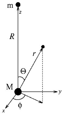
FIG. 2.: The adopted coordinate system. The black hole $M$ is at the origin and the companion $m$ is on the $z$ axis.

We will now improve the previous treatment by incorporating the tidal field of the companion star in a fully relativistic fashion. To do this, we treat the effect of the companion as a small perturbation on a Schwarzschild background. By assuming that the companion orbits at a much greater distance from the black hole than the test particles, and hence moves with a much smaller angular velocity, we can work in the quasi-static approximation. We place the companion on the $z$ axis of our spherical polar coordinate system centered on the black hole (see Figure 2). We follow Regge and Wheeler [11] and divide the linear metric perturbations into independent “even” and “odd” components according to

$$g_{\mu\nu}\ =\ g_{\mu\nu}(S)+h_{\mu\nu}(\mbox{odd})+h_{\mu\nu}(\mbox{even})\,,$$ (9)

where $g_{\mu\nu}(S)$ is the usual Schwarzschild metric. In the appropriate gauge, Regge and Wheeler found that the odd perturbations may be written as

$$\begin{array}[]{l}h_{\mu\nu}(\mbox{odd})\ =\ \pmatrix{0&0&0&h_{0}(r)\cr 0&0&0&h_{1}(r)\cr 0&0&0&0\cr h_{0}(r)&h_{1}(r)&0&0\cr}\times\hskip 100.4338pt\cr\vrule width=0.0pt,height=15.0pt\hskip 148.7975pt\sin\theta{\partial\over\partial\theta}Y_{L0}(\theta)\times e^{(i\omega t)}\,.\cr\end{array}$$ (10)

Likewise, the even perturbations may be written, after simplifying gauge transformations, as

$$\begin{array}[]{l}h_{\mu\nu}(\mbox{even})=\hskip 186.32007pt\\ \vrule width=0.0pt,height=35.0pt\hskip 52.96791pt\pmatrix{\scriptstyle H_{0}(r)(1-2M/r)&\scriptstyle H_{1}(r)&\scriptstyle 0&\scriptstyle 0\cr\scriptstyle H_{1}(r)&\vrule width=0.0pt,height=12.0pt{\scriptstyle H_{2}(r)\over(1-2M/r)}&\scriptstyle 0&\scriptstyle 0\cr\scriptstyle 0&\scriptstyle 0&\scriptstyle r^{2}K(r)&\scriptstyle 0\cr\scriptstyle 0&\scriptstyle 0&\scriptstyle 0&\scriptstyle r^{2}\sin^{2}\theta K(r)\cr}\times\hskip 52.96791pt\\ \vrule width=0.0pt,height=15.0pt\hskip 175.77322ptY_{L0}(\theta)\times e^{(i\omega t)}\,.\\ \end{array}$$ (11)

We now proceed to solve Einstein’s equations to first order in the perturbation functions as in Zerilli  [12], using a delta function (point) source for the companion. We first find solutions to the homogeneous equations away from the companion and then use the inhomogeneous source terms to match these solutions. Setting $\omega=0$ to comply with our quasi-static approximation, Zerilli’s equations reduce to

$$h_{1}=H_{1}=0;\ \ \ \ \ H_{0}\ =\ H_{2}\equiv H\,$$ (12)

$$\begin{array}[]{l}\displaystyle{d^{2}h_{0}\over dr^{2}}+\left[{4M\over r^{2}}-{L(L+1)\over r}\right]{h_{0}\over r-2M}=\hskip 116.6719pt\\ \vrule width=0.0pt,height=15.0pt\hskip 137.13824pt-8\pi r\left[{1\over 2}L(L+1)\right]^{-1/2}Q_{L}^{(0)}\,,\\ \end{array}$$ (13)

$$\begin{array}[]{l}\bigl{(}1-{2M\over r}\bigr{)}^{2}{d^{2}K\over dr^{2}}+\bigl{(}1-{2M\over r}\bigr{)}\bigl{(}3-{5M\over r}\bigr{)}{1\over r}{dK\over dr}\hskip 81.75421pt\\ \vrule width=0.0pt,height=15.0pt\hskip 20.53552pt-\bigl{(}1-{2M\over r}\bigr{)}^{2}\ {1\over r}\ {dH\over dr}-\bigl{(}1-{2M\over r}\bigr{)}{1\over r^{2}}(H-K)\hskip 20.53552pt\hskip 20.53552pt\hskip 20.53552pt\\ \vrule width=0.0pt,height=15.0pt\hskip 65.4412pt-\bigl{(}1-{2M\over r}\bigr{)}{1\over 2r^{2}}L(L+1)(H+K)=8\pi A_{L}^{(0)}\,,\\ \end{array}$$ (14)

$$\hskip 14.69351pt-{1-M/r\over r-2M}{dK\over dr}+{1\over r}{dH\over dr}+{2-L(L+1)\over 2r(r-2M)}(H-K)=8\pi A_{L}\,.\hskip 14.69351pt$$ (15)

In the above equations, $Q_{L}$, $A_{L}$, and $A_{L}^{(0)}$ represent components of the stress-energy tensor. For a point source companion moving along a Schwarzschild geodesic, these terms are given in Appendix E of Zerilli  [12]. From Zerilli’s tabulation of the source terms, one sees that all the source terms go to zero in the static limit except for $A_{L}^{(0)}$, i.e. $T_{00}$.

Homogeneous solutions may be found analytically for both the even and odd perturbations. Regge and Wheeler show that, in the large $r$ limit (where the companion resides), there is one solution for $h_{0}$ varying like $r^{-L}$, and another varying like $r^{L+1}$. Since there is no source term for $h_{0}$ ($Q_{L}=0$), the only way that both $h_{0}$ and its first derivative can be continuous and regular everywhere is to require $h_{0}=0$. Therefore, there is no contribution from odd parity perturbations.

The static solutions for $H$ and $K$ are found both by Regge and Wheeler [11] and by Zerilli [12] in terms of hypergeometric functions. We are interested in the lowest order nontrivial contribution, the quadrupole piece, generated by the companion, so we restrict our attention to the $L=2$ perturbation. Inside the orbit of the companion, the solution which is regular at the horizon is

$$\begin{array}[]{ll}\displaystyle H\ =\ \kappa_{1}r(r-2M)&\approx\kappa_{1}r^{2}\\ \displaystyle K\ =\ \kappa_{1}(r^{2}-2M^{2})&\approx\kappa_{1}r^{2}\,,\end{array}$$ (16)

where the last equality in each equation above holds at large $r\gg M$ and $\kappa_{1}$ is a constant to be determined by matching at the companion. These equations may be verified by direct substitution into Eq. (14) or (15). Outside the orbit of the companion, the perturbation is given by the solution regular at infinity,

$$\begin{array}[]{ll}H&=\ \kappa_{2}\Bigl{[}{2M(2M^{3}+4M^{2}r-9Mr^{2}+3r^{3})\over(2M-r)r}\\ &\hskip 90.0pt+{3r^{2}(r-2M)^{2}\ln(1-2M/r)\over(2M-r)r}\Bigr{]}\\ &\approx\kappa_{2}r^{-3}\\ &\\ K&=\ \kappa_{2}M^{2}\bigl{[}-6+{{4M}\over{r}}-{{6r}\over{M}}-{{3r^{2}\ln(1-2M/r)}\over{M^{2}}}\\ &\vrule width=0.0pt,height=15.0pt\hskip 120.0pt+6\ln(1-2M/r)\bigr{]}\\ &\approx\kappa_{2}r^{-3}\,,\end{array}$$ (17)

where the last equality in each equation again holds at large $r\gg M$ and $\kappa_{2}$ is another constant to be determined by matching.

Now we determine the two constants by matching the solutions at the radius of orbit of the companion, $R$. Because $A_{L}^{(0)}$, the source term of (14), does not go to zero in the quasi-static case, $\kappa_{1}$ and $\kappa_{2}$ do not vanish, as was the case for the odd parity solutions. Taking $R\gg M$ as required by the quasi-static approximation, we use the asymptotic expressions in equations (16) and (17) for the matching. Requiring that $K$ be continuous across $R$ then yields our first condition

$$\kappa_{1}R^{2}=\kappa_{2}R^{-3}~{}~{}\Rightarrow~{}~{}\kappa_{2}=R^{5}\kappa_{1}\,.$$ (18)

The second condition may be found in either of two ways. First, one may integrate Equation (14) across the source to obtain a jump condition relating difference in the first derivative of $K$ on either side of $r=R$ to the source strength. Alternatively, one may compute $\kappa_{1}$ directly by taking the Newtonian limit of $H$ and matching it to the Newtonian tidal potential. Either way, one obtains $\kappa_{1}={{m}\over{R^{3}}}4\sqrt{\pi/5}$. Thus, $h_{00}$, for example, is

$$\begin{array}[]{l}h_{00}=(1-2M/r)(r^{2}-2Mr)\kappa_{1}Y_{20}(\theta)\hskip 89.55887pt\\ \vrule width=0.0pt,height=15.0pt\hskip 71.45096pt=(1-2M/r)(r^{2}-2Mr){m\over R^{3}}(3\cos^{2}\theta-1)\,.\\ \end{array}$$ (19)

From (19), one can immediately verify that the metric derived above has the correct Newtonian limit—the potential reduces to the classic Hill potential. This solution for the even parity solutions was first discovered by Moeckel [17].

The entire metric may now be written out, defining $P\equiv P_{2}(\cos\theta)=3\cos^{2}\theta-1$:

$$\begin{array}[]{l}ds^{2}=\Bigl{[}-\bigl{(}1-{2M\over r}\bigr{)}+{m\over R^{3}}P(r-2M)^{2}\Bigr{]}dt^{2}\hskip 91.01758pt\\ \vrule width=0.0pt,height=15.0pt\hskip 65.16167pt+\Bigl{[}\bigl{(}1-{2M\over r}\bigr{)}^{-1}+{m\over R^{3}}Pr^{2}\Bigr{]}dr^{2}\hskip 65.16167pt\\ \vrule width=0.0pt,height=15.0pt\hskip 116.68953pt+\Bigl{[}r^{2}+{m\over R^{3}}Pr^{2}(r^{2}-2M^{2})\Bigr{]}d\Omega^{2}\,.\end{array}$$ (20)

We note that the perturbed spacetime (20) furnishes another example supporting the conjecture of Bekenstein  [13] that the horizon area of a near-equilibrium black hole is an adiabatic invariant (see Appendix).

To compare with the hybrid-PN treatment, we transform to harmonic coordinates by replacing the areal radial coordinate, $r$, with the harmonic radius, $r_{h}=r-M$. Dropping the subscript, we obtain in harmonic coordinates

$$\begin{array}[]{l}ds^{2}\ =\displaystyle-{r-M\over r+M}dt^{2}+{r+M\over r-M}dr^{2}+(r+M)^{2}d\Omega^{2}\hskip 48.01654pt\\ \hskip 24.41496pt\hskip 24.41496pt\hskip 24.41496pt\vrule width=0.0pt,height=15.0pt\displaystyle+{m\over R^{3}}P\bigl{[}(r-M)^{2}dt^{2}+(r+M)^{2}dr^{2}\hskip 24.41496pt\\ \hskip 97.2967pt\displaystyle+(r+M)^{2}(r^{2}+2rM-M^{2})d\Omega^{2}\bigr{]}\,.\\ \end{array}$$ (21)

Obtaining the geodesic equations in this spacetime up to first order in the tidal expansion parameter ${mr^{2}\over R^{3}}$, we find the equations of motion for a test particle near the black hole to be

$$\begin{array}[]{l}\displaystyle\ddot{r}={3M\dot{r}^{2}\over r^{2}-M^{2}}-{M(r-M)\over(r+M)^{3}}+(r-M)\Omega^{2}\hskip 106.732pt\\ \hskip 25.01457pt\vrule width=0.0pt,height=15.0pt+{m\over R^{3}}P\Big{[}-3r\dot{r}^{2}+(r+2M){(r-M)^{2}\over(r+M)^{2}}\hskip 25.01457pt\hskip 25.01457pt\hskip 25.01457pt\\ \hskip 55.42851pt\vrule width=0.0pt,height=15.0pt+(r-M)(r^{2}+4rM+M^{2})\Omega^{2}\Big{]}\hskip 55.42851pt\\ \hskip 164.1127pt\vrule width=0.0pt,height=15.0pt-{m\over R^{3}}2(r^{2}-M^{2}){dP\over d\theta}\dot{\theta}\dot{r}\\ \\ \ddot{\theta}={4M-2r\over r^{2}-M^{2}}\dot{\theta}\dot{r}+\cos\theta\sin\theta\dot{\phi}^{2}\hskip 135.89671pt\\ \hskip 37.47939pt\vrule width=0.0pt,height=15.0pt+{m\over R^{3}}P[-2(M+2r)\dot{\theta}\dot{r}]\hskip 37.47939pt\hskip 37.47939pt\hskip 37.47939pt\\ \hskip 54.5325pt\vrule width=0.0pt,height=15.0pt+{m\over R^{3}}{dP\over d\theta}{1\over 2}\Big{[}-(3r^{2}+2rM-3M^{2})\dot{\theta}^{2}\hskip 54.5325pt\\ \hskip 71.04018pt\vrule width=0.0pt,height=15.0pt+(r^{2}+2rM-M^{2})\sin^{2}\theta\ \dot{\phi}^{2}+{(r-M)^{2}\over(r+M)^{2}}+\dot{r}^{2}\Big{]}\\ \\ \ddot{\phi}\ =\ {4M-2r\over r^{2}-M^{2}}\dot{\phi}\dot{r}-2\cot\theta\ \dot{\theta}\dot{\phi}-2{m\over R^{3}}P(M+2r)\dot{\phi}\dot{r}\hskip 59.08667pt\\ \hskip 131.86513pt\vrule width=0.0pt,height=15.0pt-2{m\over R^{3}}{dP\over d\theta}(r^{2}+rM-M^{2})\dot{\theta}\dot{\phi}\,,\\ \end{array}$$ (22)

where dot denotes differentiation with respect to Schwarzschild coordinate time, and $\Omega^{2}=\dot{\theta}^{2}+\sin^{2}\theta\dot{\phi}^{2}$. To avoid coordinate singularities, it is convenient to integrate (22) in Cartesian coordinates. To facilitate an otherwise tedious transformation, we first rewrite the equations of motion in 3-vector form. We make the identification

$$\begin{array}[]{lll}{\bf\ddot{r}}=&&(\ddot{r}-r\dot{\phi}^{2}\sin^{2}\theta-r\dot{\theta}^{2}){\partial\over\partial r}\\ \vrule width=0.0pt,height=15.0pt&+&(\ddot{\theta}+(2\dot{r}\dot{\theta}-r\dot{\phi}^{2}\sin\theta\cos\theta)/r){\partial\over\partial\theta}\\ \vrule width=0.0pt,height=15.0pt&+&(\ddot{\phi}+(2\dot{r}\dot{\phi}\sin\theta+2r\dot{\theta}\dot{\phi}\cos\theta)/(r\sin\theta)){\partial\over\partial\phi}\,,\\ \end{array}$$ (23)

a vector which we have constructed to be the same as the Newtonian 3-acceleration in spherical coordinates and we know transforms to $(\ddot{x},\ddot{y},\ddot{z})$ in Cartesian coordinates. Identifying the velocity 3-vector ${\bf v}=(\dot{r},\dot{\theta},\dot{\phi})$ in the spherical coordinate basis and setting ${\bf r}=r{\partial\over\partial r}$ allows us to write (22) in the compact form 3-vector form

$$\begin{array}[]{l}\displaystyle{\bf\ddot{r}}=-{M\over r^{2}}[A{\bf e_{r}}+B{\bf v}]\hskip 166.03926pt\\ \displaystyle\hskip 117.16147pt\vrule width=0.0pt,height=15.0pt+{m\over R^{3}}\left[\alpha\left({3{\bf r}\cdot{\bf R}\over R^{2}}{\bf R}-{\bf r}\right)+\beta{\bf v}+\gamma{\bf e_{r}}\right]\,,\\ \end{array}$$ (24)

where $A$ and $B$ are again given by Eqs. (2) and  (3). The quantities $\alpha$, $\beta$, and $\gamma$ are given by

$$\begin{array}[]{l}\displaystyle\alpha=(r^{2}+2rM-M^{2}){v^{2}-\dot{r}^{2}\over r^{2}}+\dot{r}^{2}+{(r-M)^{2}\over(r+M)^{2}}\hskip 79.18727pt\\ \\ \displaystyle\beta=-2(3\cos^{2}\Theta-1)(M+2r)\dot{r}\hskip 118.57393pt\\ \displaystyle\hskip 111.90459pt\vrule width=0.0pt,height=15.0pt+12\cos\Theta\sin\Theta(r^{2}+rM-M^{2})\dot{\Theta}\\ \\ \displaystyle\gamma=(3\cos^{2}\Theta-1)\Biggl{[}2M\bigl{(}\dot{r}^{2}+{(r-M)^{2}\over(r+M)^{2}}\bigr{)}\hskip 88.32779pt\\ \displaystyle\hskip 32.60452pt\hskip 32.60452pt\hskip 32.60452pt\vrule width=0.0pt,height=15.0pt+M(r^{2}-2rM-M^{2}){v^{2}-\dot{r}^{2}\over r^{2}}\Biggr{]}\hskip 32.60452pt\\ \displaystyle\hskip 153.64116pt\vrule width=0.0pt,height=15.0pt-12rM\dot{r}\dot{\Theta}\cos\Theta\sin\Theta\,,\\ \end{array}$$ (25)

where $\Theta$ is the angle between $\bf r$ and ${\bf R}$. It is now straightforward to write out the Cartesian components of Eq. (24). To incorporate the (slow) inspiral of the companion in the context of our quasi-static approximation, we treat ${\bf R}={\bf R(t)}$ in Eq. (24) as a parameter, which is slowly evolved in accord with Eqs. (6), (7) and (8).

The leading terms independent of the companion $m$ are identical in both (24) and (1), a result which is consistent with the adoption of hybrid equations in the PN analysis. The tidal term in (24) reduces to the lowest-order Newtonian expression used in (1) in the weak-field, slow-velocity limit where $v\ll 1$, $M/r\ll 1$. Since the test particles orbit close to the hole, the relativistic tidal expression will indeed cause departures from the motion predicted by the Newtonian tidal term.

B Numerical Implementation

A spherical swarm identical to the one evolved with the hybrid-PN equations of motion was evolved with Eq.(24). Because collapse occurs later in this simulation, the swarm was evolved until $R/M=26.30$. The results are summarized in Figures 3 – 5. In Figure 3, the mean cluster radius is computed once again and compared to the hybrid-PN result. The qualitative nature of the evolution is the same, and the existence of a crushing instability is evident. The main effect of the new relativistic terms is to delay the collapse until the perturber gets somewhat closer to the hole. In particular, of 20,000 particles, 16,324 fell into the hole (81.6 %) by the time the companion reached $R/M=26.30$, a slightly smaller percentage than in the hybrid-PN simulation. Once again, the compact cluster is observed to be stable in isolation, but driven to collapse by the presence of a sufficiently strong tidal perturbation.

FIG. 3.: Evolution of the cluster in the Schwarzschild perturbation treatment. The mean radius of the 20,000 test-particles in the initially spherical swarm is plotted as a function of the tidal companion radius in the top figure and as a function of coordinate time in the bottom figure. In the top figure we compare the results found for our two treatments; the behavior is qualitatively similar, but the crushing effect occurs slightly later in the fully relativistic, Schwarzschild perturbation treatment.

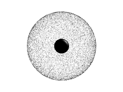
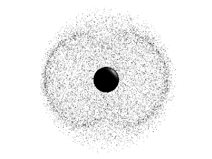
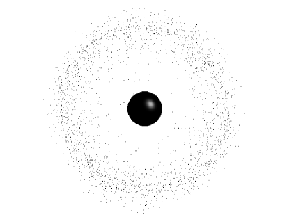
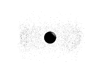
A B $t/M=0$ $t/M=1.18\times 10^{5}$ $t/M=1.22\times 10^{5}$

FIG. 4.: Snapshots of the cluster swarm at selected times during the binary inspiral. In $A$ we show the view looking down along the $z$-axis, which is perpendicular to the orbital plane of the companion; in $B$ we show the view looking along the $x$-axis, which lies in the orbital plane of the companion. For the top frame the companion is at $R/M=60$; for the middle frame the companion is at $R/M=30.7$; for the bottom frame the companion is at $R/M=26.30$.

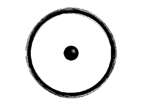
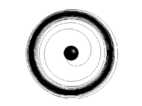
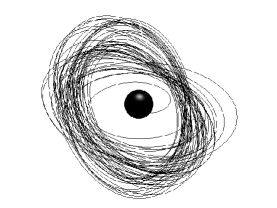
             a b c

FIG. 5.: Test-particle trajectories about the black hole during the inspiral of the binary companion from $R/M=60$ to $R/M=26.30$. Frame (a) shows the orbit of a particle moving in the orbital plane of the companion; it is not captured by the time the integrations terminate. Frame (b) shows the capture of a particle initially orbiting in a plane perpendicular to the companion plane. Frame (c) shows the precession and capture of a particle initially orbiting at an angle of $45^{o}$ to the companion plane.

As the geodesic equations in the perturbative relativistic treatment are derived from a self-consistent Lagrangian, they satisfy strict conservation laws even in the presence of a companion, assuming it is stationary. These conservation laws provide a means of testing our code and particle integration scheme. For example, if the companion is fixed at an arbitrary position on the z-axis, the perturbed Schwarzschild spacetime (21) admits two Killing vectors, $\partial\over\partial t$ and $\partial\over\partial\phi$, yielding conservation of particle energy $p_{t}$ and angular momentum $p_{\phi}$, even for large tidal fields. Given that we linearize the tidal field and retain only the lowest order terms in $m$ in our equations of motion (24), energy and angular momentum conservation are no longer exact. However, we have tested our code and have shown that it reliably obeys these conservation laws to the required order.

The evolution of the swarm is depicted in Figure 4, where snapshots of the cluster are shown at three different times from two different viewing angles. By the end of the simulation, the original spherical swarm is reduced to a sparse cylindrical band of particles whose axis is perpendicular to the orbital plane of the companion. Apparently, particle orbits at small inclination angles to this plane are more stable than those which are perpendicular, a result already noted in  [1]. This feature is evident in Figure 5, which plots the trajectories of three representative particles. The simulation confirms that gravitational collapse can be induced in a collisionless cluster by the tidal field of a binary companion.

Adiabatic Invariance of the Horizon Area

Bekenstein [13] has argued recently that the horizon area of a near-equilibrium black hole is an adiabatic invariant. Using the focusing equation, he derives the following conditions which must be satisfied in order for area to remain fixed:

$$T_{\alpha\beta}l^{\alpha}l^{\beta}=0;\ \ \ \ C_{\alpha\beta\gamma\delta}l^{\alpha}m^{\beta}l^{\gamma}m^{\delta}=0\,,\ \ \mbox{(on the horizon)}$$ (26)

where $C_{\alpha\beta\gamma\delta}$ is the Weyl conformal tensor, and $l^{\alpha}$ and $m^{\alpha}$ are legs of the Newman-Penrose tetrad ($l^{\alpha}$ are tangents to the null generators of the event horizon). For our quasi-static scenario in which the companion undergoes a very slow inward spiral, there is no matter and and essentially no wave flux at the horizon, so both conditions (26) hold. (Other situations in which adiabatic invariance has been demonstrated are discussed in [13] and [18].) We may use our metric in Schwarzschild coordinates (20) to verify explicitly that in accord with Bekenstein’s conjecture, the horizon area remains invariant in our model as the companion is brought in slowly from large distance.

First, rewrite (20) in Kruskal-Szekeres coordinates, ignoring angular terms, reintroducing areal coordinate $r$ and defining $\kappa={m\over R^{3}}$,

$$\begin{array}[]{l}\displaystyle ds^{2}={32M^{3}\over r}e^{-r/2M}\Bigg{\{}-dv^{2}+du^{2}\hskip 123.59404pt\\ \displaystyle\hskip 38.27226pt\vrule width=0.0pt,height=15.0pt+{2P\kappa r\over M}e^{-r/2M}\Big{[}(u^{2}+v^{2})(du^{2}+dv^{2})-4uv\,du\,dv\Big{]}\Bigg{\}}\,.\\ \end{array}$$ (27)

Note that this metric agrees with that derived by Vishveshwara [19] for general even perturbations of Schwarzschild in Kruskal coordinates. Null geodesics are found by setting $ds^{2}=0$, for which

$$\begin{array}[]{l}\displaystyle{du\over dv}={{8uv\kappa Pr\over M}e^{-r/2M}\over 2(1+(u^{2}+v^{2}){2\kappa Pr\over M}e^{-r/2M})}\hskip 122.45064pt\\ \displaystyle\hskip 65.9508pt\vrule width=0.0pt,height=35.0pt\pm{\sqrt{{(8uv\kappa Pr)^{2}\over M^{2}}e^{-r/M}-4\Big{[}(u^{2}+v^{2})^{2}{(2\kappa Pr)^{2}\over M^{2}}e^{-r/M}-1\Big{]}}\over 2\Big{[}1+(u^{2}+v^{2}){2\kappa Pr\over M}e^{-r/2M}\Big{]}}\,.\\ \end{array}$$ (28)

Direct substitution verifies that (28) is satisfied by $u=\pm v$, $r(t)=2M$. Therefore, the horizon on the perturbed black hole remains at $2M$. The surface area of a shell of constant radius is given by

$$A=\int_{0}^{2\pi}\!\!\!\!\!\int_{0}^{\pi}\sqrt{g_{\theta\theta}g_{\phi\phi}}d\theta d\phi=4\pi r^{2}\,.$$ (29)

Due to the orthogonality of Legendre polynomials ($P_{2}$ and $P_{0}$ in this case), the quadrupole perturbations in the angular piece of metric (20) do not change areas of shells. Therefore, the area of the spherical shell $r=2M$, the location of the horizon, remains constant.

Hartle  [20] has studied the effect of tidal fields from more general stationary sources on the horizon area of slowly rotating black holes. In the limit of a nonrotating black hole, his analysis gives a vanishing time rate of change for the area, consistent with our explicit calculation above.

ACKNOWLEDGMENTS

It is a pleasure to thank A.M. Abrahams, T.W. Baumgarte and N.J. Cornish for stimulating discussions and useful suggestions. We are also grateful to K. Alvi, L. Burko, and Y.T. Liu for pointing out to us a typo in equation (7) in an earlier draft. The Undergraduate Research Team in theoretical astrophysics and general relativity (M. Duez, E. Engelhard, J. Fregeau and K. Huffenberger) gratefully acknowledges support from the Departments of Physics and Astronomy at the University of Illinois at Urbana-Champaign (UIUC). Much of the calculation and visualization were performed at the National Center for Supercomputing Applications at UIUC. This paper was supported in part by NSF Grant AST 96-18524 and NASA Grant NAG 5-7152 to UIUC.

REFERENCES

- [1] S.L. Shapiro, Phys. Rev. D. 57, 908 (1998).
- [2] J.R. Wilson and G.J. Mathews, Phys. Rev. Lett. 75, 4161 (1995); J.R. Wilson, G.J. Mathews and P. Maronetti, Phys. Rev. D 54, 1317 (1996); G.J. Mathews and J.R. Wilson, Astrophys. J. 482, 929 (1997).
- [3] D. Lai, F.A. Rasio and S.L. Shapiro, Astrophys. J. Supp. 88, 205 (1993).
- [4] D. Lai, Phys. Rev. Lett. 76, 4878 (1996); A.D. Wiseman, Phys. Rev. Lett. 79, 1189 (1997); P.R. Brady and S.A. Hughes, Phys. Rev. Lett. 79, 1186 (1997).
- [5] J.C. Lombardi, F.A. Rasio and S.L. Shapiro, Phys. Rev. D. 56 3416 (1997); M. Shibata, Prog. Theo. Phys. 96, 317 (1996); K. Taniguchi and M. Shibata, Phys. Rev. D. 56 798 (1997), ibid, 56, 811 (1997); M. Shibata, K. Oohara and T. Nakamura, Prog. Theor. Phys. 98, 1081 (1997).
- [6] K.S. Thorne, Phys. Rev. D. 58, 124031 (1998); E.E. Flanagan, Phys. Rev. D. 58, 124030 (1998); ibid, Phys. Rev. Lett. 82, 1354 (1999).
- [7] M. Shibata, T.W. Baumgarte and S.L. Shapiro, Phys. Rev. D, 58, 23002 (1998).
- [8] T.W. Baumgarte, G.B. Cook, M.A. Scheel, S.L. Shapiro and S.A. Teukolsky, Phys. Rev. Lett. 79, 1182 (1997); ibid, Phys. Rev. D 57, 6181 (1998); ibid, Phys. Rev. D 57 7299 (1998).
- [9] S. Bonazzola, E. Gourgoulhon and J.-A. Marck, Phys. Rev. Lett. 82, 892 (1999).
- [10] L.E. Kidder, C.M. Will and A.G. Wiseman, Phys. Rev. D. 47, 3281 (1993).
- [11] T. Regge and J.A. Wheeler, Phys. Rev. 108, 1063 (1957).
- [12] F.J. Zerilli, Phys. Rev. D. 2, 2141 (1970).
- [13] J.D. Bekenstein, gr-qc/9805045.
- [14] C.W. Lincoln and C.M. Will, Phys. Rev. D. 42, 1123 (1990).
- [15] Our inspiral approximation is performed in the same spirit as the hybrid approximation, where complete PN consistency is sacrificed in order to insure that the equations recover some essential dynamical behavior arising at higher order.
- [16] W.H. Press, S.A. Teukolsky, W.T. Vetterling and B.P. Flannery, Numerical Recipes (Cambridge University Press, Cambridge, 1992).
- [17] R. Moeckel, Commun. Math. Physics. 150, 415 (1992).
- [18] A.E. Mayo, Phys. Rev. D. 58, 104007 (1998).
- [19] C.V. Vishveshwara, Phys. Rev. D. 1, 2870 (1970).
- [20] J.B. Hartle, Phys. Rev. D. 8, 1010 (1973).