Non-linear Evolution of Rotating Relativistic Stars

Abstract

We present first results of the non-linear evolution of rotating relativistic stars obtained with an axisymmetric relativistic hydrodynamics code in a fixed spacetime. As initial data we use stationary axisymmetric and perturbed configurations. We find that, in order to prevent (numerical) angular momentum loss at the surface layers of the star a high-resolution grid (or a numerical scheme that retains high order at local extrema) is needed. For non-rotating stars, we compute frequencies of radial and non-radial small-amplitude oscillations, which are in excellent agreement with linear normal mode frequencies computed in the Cowling approximation. As a first application of our code, quasi-radial modes of rapidly rotating relativistic stars are computed. By generalizing our numerical code to 3-D, we plan to study the evolution and non-linear dynamics of toroidal oscillations ($r$-modes) of rapidly rotating neutron stars, which are a promising source of gravitational waves.

• (1) Max-Planck-Institut für Gravitationsphysik
  Albert-Einstein-Institut
  Schlaatzweg 1, D-14473, Potsdam, Germany
  

• (2) Department of Physics
  Aristotle University of Thessaloniki
  Thessaloniki 54006, Greece
  Email: niksterg@aei-potsdam.mpg.de, font@aei-potsdam.mpg.de,
  kokkotas@astro.auth.gr

1 Introduction

The numerical evolution of neutron stars in full General Relativity has been the focus of many research groups in recent years [1, 2, 3, 4]. So far, these studies have been limited to initially non-rotating stars. However, the numerical investigation of many interesting astrophysical applications, such as the rotational evolution of proto-neutron stars and merged neutron stars or the simulation of gravitational radiation from unstable pulsation modes, requires the ability of accurate long-term evolutions of rapidly rotating stars. We thus present here the first study of hydrodynamical evolutions of rotating neutron stars in the approximation of a static spacetime. This approximation allows us to evolve relativistic matter for a much longer time than present coupled spacetime plus hydrodynamical evolution codes. Since the pulsations of neutron stars are mainly a hydrodynamical process, the exclusion of the spacetime dynamics has only a limited effect and allows for qualitative conclusions to be drawn.

The rotational evolution of neutron stars can be affected by several instabilities (see [5] for a recent review). If hot protoneutron stars are rapidly rotating, they can undergo a dynamical bar-mode instability [6]. When the neutron star has cooled to about $10^{10}$K after its formation, it can be subject to the Chandrasekhar-Friedman-Schutz instability [7, 8] and it becomes an important source of gravitational waves. It was recently found that the $l=m$ $r$-mode has the shortest growth time of the instability [9, 10] and it can transform a rapidly rotating newly-born neutron star to a Crab-like slowly-rotating pulsar within about a year after its formation [11, 12]. In this model, there are two important questions still to be answered [13]: What is the maximum amplitude that an unstable $r$-mode can reach (limited by nonlinear saturation) and is there any transfer of energy to other stable or unstable modes via non-linear couplings? Such questions cannot be answered by computations of normal modes of the linearized pulsation equations, but require non-linear effects to be taken into account. We therefore need to develop the capability of full non-linear numerical evolutions of rotating stars in General Relativity.

Our present 2-D (axisymmetric) code uses high-resolution shock-capturing (HRSC) finite-difference schemes for the numerical integration of the general relativistic hydrodynamic equations [14] (see [15] for a recent review of applications of HRSC schemes in relativistic hydrodynamics). In a similar context to the one presented here let us note that such schemes have been succesfully used before in the study of the numerical evolution and gravitational collapse of non-rotating neutron stars in 1-D [16]. An alternative approach, based on pseudospectral methods, has been presented in [17].

Using our code in 1-D time-evolutions we can accurately identify specific normal modes of pulsation. In 2-D the code is suitable for the evolution of rotating stars, with the additional complication of having to pay special attention to an angular momentum-loss at the (non-spherical) surface of the star, as we will show below.

2 Initial Configurations

Our initial models are fully relativistic, stationary and axisymmetric configurations, rotating with uniform angular velocity $\Omega$. The metric in quasi-isotropic coordinates [18] is

$$ds^{2}=-e^{2\nu}dt^{2}+B^{2}e^{-2\nu}r^{2}\sin^{2}\theta(d\phi-\omega dt)^{2}+e^{2\alpha}(dr^{2}+r^{2}d\theta^{2}),$$ (1)

where $\nu$, $B$, $\alpha$ and $\omega$ are metric functions (gravitational units are implied). In the non-rotating limit the above metric reduces to the metric of spherical relativistic stars in isotropic coordinates.

We assume a perfect fluid, zero-temperature equation of state (EOS), for which the energy density is a function of pressure only. The following relativistic generalization of the Newtonian polytropic EOS is chosen:

$$p = K\rho_{0}^{1+1/N}$$ (2)

$$\epsilon = \rho_{0}+Np,$$ (3)

where $p$ is the pressure, $\epsilon$ is the energy density, $\rho_{0}$ is the rest-mass density, $K$ is the polytropic constant and $N$ is the polytropic exponent.

The initial equilibrium models are computed using a numerical code by Stergioulas & Friedman [19] which follows the Komatsu, Eriguchi & Hatchisu [20] method (as modified in [21]) with some changes for improved accuracy (see [22] for a comparison with other codes). The code is freely available and can be downloaded from the following URL address: http://www.gravity.phys.uwm.edu/Code/rns.

3 Relativistic Hydrodynamic Equations

The equations of (ideal) relativistic hydrodynamics are obtained from the local conservation laws of density current, $J^{\mu}$ and stress-energy, $T^{\mu\nu}$

$$\nabla_{\mu}J^{\mu} = 0$$ (4)

$$\nabla_{\mu}T^{\mu\nu} = 0$$ (5)

with

$$J^{\mu} = \rho_{0}u^{\mu}$$ (6)

$$T^{\mu\nu} = \rho_{0}hu^{\mu}u^{\nu}+pg^{\mu\nu},$$ (7)

for a general EOS $p=p(\rho,\varepsilon)$. This choice of the stress-energy tensor limits our study to perfect fluids.

In the previous expressions $\nabla_{\mu}$ is the covariant derivative, $u^{\mu}$ is the fluid 4-velocity and $h$ is the specific enthalpy

$$h=1+\varepsilon+\frac{p}{\rho_{0}}$$ (8)

with $\varepsilon$ being the specific internal energy, related to the energy density $\epsilon$ by

$$\varepsilon=\frac{\epsilon}{\rho_{0}}-1.$$ (9)

With an appropriate choice of matter fields the equations of relativistic hydrodynamics constitute a (non-strictly) hyperbolic system and can be written in a flux conservative form, as was first shown in [23] for the one-dimensional case. The knowledge of the characteristic fields of the system allows the numerical integration to be performed by means of advanced high-resolution shock-capturing (HRSC) schemes,using approximate Riemann solvers (Godunov-type methods). The multidimensional case was studied in [24], within the framework of the 3+1 formulation. Further extensions of this work to account for dynamical spacetimes, described by the full set of Einstein’s non-vacuum equations, can be found in [1]. Fully covariant formulations of the hydrodynamic equations (i.e., not restricted to spacelike approaches) and also adapted to Godunov-type methods, are presented in [25, 26].

In the present work we use the hydrodynamic equations as formulated in [24]. Specializing for the metric given by Eq. (1), the 3+1 quantities read

$$\tilde{\alpha} = e^{\nu}$$ (10)

$$\beta_{\phi} = -\omega B^{2}e^{-2\nu}r^{2}\sin^{2}\theta$$ (11)

$$\gamma_{rr} = e^{2\alpha}$$ (12)

$$\gamma_{\theta\theta} = r^{2}e^{2\alpha}$$ (13)

$$\gamma_{\phi\phi} = B^{2}e^{-2\nu}r^{2}\sin^{2}\theta$$ (14)

where $\tilde{\alpha}$ is the lapse function (the tilde is used to avoid confussion with the metric potential $\alpha$) and $\beta_{\phi}$ is the azimuthal shift.

The hydrodynamic equations are written as a first-order flux conservative system of the form

$$\frac{\partial{\bf u}}{\partial t}+\frac{\partial\tilde{\alpha}{\bf f}^{r}}{\partial r}+\frac{\partial\tilde{\alpha}{\bf f}^{\theta}}{\partial\theta}={\bf s}$$ (15)

where ${\bf u},{\bf f}^{r},{\bf f}^{\theta}$ and ${\bf s}$ are, respectively, the state vector of evolved quantities, the radial and polar fluxes and the source terms. More precisely, they take the form

$${\bf u} = (D,S_{r},S_{\theta},S_{\phi},\tau)$$ (16)

$${\bf f}^{r} = (Dv^{r},S_{r}v^{r}+p,S_{\theta}v^{r},S_{\phi}v^{r},(\tau+p)v^{r})$$ (17)

$${\bf f}^{\theta} = (Dv^{\theta},S_{r}v^{\theta},S_{\theta}v^{\theta}+p,S_{\phi}v^{\theta},(\tau+p)v^{\theta}).$$ (18)

The source terms can be decomposed in the following way

$${\bf s}=\tilde{\alpha}{\bf s}^{\star}-\tilde{\alpha}{\bf f}^{r}\frac{\partial\log\sqrt{\gamma}}{\partial r}-\tilde{\alpha}{\bf f}^{\theta}\frac{\partial\log\sqrt{\gamma}}{\partial\theta}$$ (19)

with $\gamma=\det\gamma_{ij}$ and

$${\bf s}^{\star}=\left(0,T^{\mu\nu}\left[\frac{\partial g_{\nu j}}{\partial x^{\mu}}-\Gamma^{\delta}_{\mu\nu}g_{\delta j}\right],\tilde{\alpha}\left[T^{\mu t}\frac{\partial\log\tilde{\alpha}}{\partial x^{\mu}}-T^{\mu\nu}\Gamma^{t}_{\mu\nu}\right]\right)$$ (20)

with $j=r,\theta,\phi$. The definitions of the evolved quantities in terms of the “primitive” variables ($\rho,v_{j},\varepsilon$) are

$$D = \rho_{0}W$$ (21)

$$S_{j} = \rho_{0}hW^{2}v_{j}$$ (22)

$$\tau = \rho_{0}hW^{2}-p-D$$ (23)

where $W$ is the relativistic Lorentz factor

$$W\equiv\tilde{\alpha}u^{t}=\frac{1}{\sqrt{1-v^{2}}}$$ (24)

with $v^{2}=\gamma_{ij}v^{i}v^{j}$. The 3-velocity components are obtained from the spatial components of the 4-velocity in the following way

$$v^{i}=\frac{u^{i}}{W}+\frac{\beta^{i}}{\tilde{\alpha}}.$$ (25)

Explicit expressions for the non-vanishing Christoffel symbols for metric (1), appearing in the source terms of the hydrodynamic equations, are presented in [27].

4 Numerical Methods

As stated before, our numerical integration of system (15) is based on Godunov-type methods (also known as HRSC schemes). In a HRSC scheme, the knowledge of the characteristic fields (eigenvalues) of the equations, together with the corresponding eigenvectors, allows for accurate integrations, by means of either exact or approximate Riemann solvers, along the fluid characteristics. These solvers, which constitute the kernel of our numerical algorithm, compute, at every interface of the numerical grid, the solution of local Riemann problems (i.e., the simplest initial value problem with discontinuous initial data). Hence, HRSC schemes automatically guarantee that physical discontinuities appearing in the solution, e.g., shock waves, are treated consistently (the shock-capturing property). HRSC schemes are also known for giving stable and sharp discrete shock profiles. They have also a high order of accuracy, typically second order or more, in smooth regions of the solution.

We perform the time update of system (15) according to the following conservative algorithm:

$${\bf u}_{i,j}^{n+1}={\bf u}_{i,j}^{n} - \frac{\Delta t}{\Delta r}(\widehat{{\bf f}}_{i+1/2,j}-\widehat{{\bf f}}_{i-1/2,j})$$ (26)

$$- \frac{\Delta t}{\Delta\theta}(\widehat{{\bf g}}_{i,j+1/2}-\widehat{{\bf g}}_{i,j-1/2})+\Delta t{\bf s}_{i,j}\,.$$

Index $n$ represents the time level and the time (space) discretization interval is indicated by $\Delta t$ ($\Delta r,\Delta\theta$). The “hat” in the fluxes is used to denote the so-called numerical fluxes which, in a HRSC scheme, are computed according to some generic flux-formula, of the following functional form (suppressing index $j$):

$$\widehat{{\bf f}}_{i\pm{1\over 2}}=\frac{1}{2}\left({\bf f}({\bf u}_{i\pm{1\over 2}}^{L})+{\bf f}({\bf u}_{i\pm{1\over 2}}^{R})-\sum_{\alpha=1}^{5}\mid\widetilde{\lambda}_{\alpha}\mid\Delta\widetilde{\omega}_{\alpha}\widetilde{r}_{\alpha}\right)\,.$$ (27)

Notice that the numerical flux is computed at cell interfaces ($i\pm 1/2$). Indices $L$ and $R$ indicate the left and right sides of a given interface. Quantities $\lambda$, $\Delta\omega$ and $r$ denote the eigenvalues, the jump of the characteristic variables and the eigenvectors, respectively, computed at the cell interfaces according to some suitable average of the state vector variables. Generic expressions for the characteristic speeds and eigenfields can be found in [1]. Our code has the ability of using different approximate Riemann solvers: the Roe solver [28], widely employed in fluid dynamics simulations, with arithmetically averaged states and the Marquina solver [29], which has been extended to Relativity in [30]. The computations presented here were obtained using Marquina’s scheme.

A technical remark: the equilibrium star is supplemented by a low-density uniform atmosphere, which is necessary for computing non-singular solutions of the hydrodynamic equations everywhere in the computational domain. After each time-step we reset the atmosphere’s density and pressure to their initial values, avoiding unwanted accretion of matter onto the star. The influence of the atmosphere is thus restricted to the surface grid-cells.

5 Pulsations of Non-rotating Stars

Since our code uses spherical polar coordinates, it can also be employed to study the evolution of non-rotating stars in 1-D. In the evolution of initially static non-rotating stars, we observe the following properties (note that our numerical grid is Eulerian):

1. Small-amplitude radial pulsations are triggered by the truncation errors of the finite-differencing scheme.

2. The radial pulsations are dominated by a set of discrete frequencies, which correspond to the normal modes of pulsation of the star.

3. The numerical viscosity of the finite-difference scheme damps the pulsations and the damping is stronger for the higher frequency modes.

4. The presence of a constant density atmosphere affects the finite differencing at the surface grid-cells, which increases the numerical damping of pulsations and also causes a continuous but very small drifting of the density distribution.

The initial amplitude of the radial pulsations and the small drift in density converge to zero at a second order rate with increasing resolution. The value of the density in the atmosphere region has a large effect on the damping of the pulsations. If it is too large, the damping is strong. To minimize this effect, we typically set the density of the atmosphere equal to $10^{-6}$ times the density of the last grid point inside the star.

5.1 1-D evolutions

We study the numerical evolution of a nonrotating $N=1.5$ relativistic polytrope with $M/R=0.056$. The star is immediately set into radial pulsation, triggered by the finite difference truncation errors. The time-evolution of the radial velocity $v_{r}$, computed at 25% of the star radius using a grid of 400 zones, is shown in Fig. 1. The vertical axis is dimensionless ($c=G=M_{\odot}=1$). The radial velocity is initially a very complex function of time. As we will show next, the pulsation consists mainly of a superposition of normal modes of oscillation of the fluid. The high frequency normal modes are damped quickly and after 20ms the star pulsates mostly in lowest frequency modes. Because these oscillations are caused only by the truncation errors, the magnitude of the radial velocity is extremely small. As shown in Fig. 1 it is only a few times larger than the non-zero residual velocity around which the star is oscillating. This residual velocity converges to zero as second order with increased resolution.

Figure 1: Evolution of the radial velocity of an initially static, non-rotating star, caused by the truncation errors of the finite-difference scheme. The radial pulsations are mainly a superposition of normal modes of the star.

The small-amplitude radial pulsations in the non-linear, fixed spacetime evolutions correspond to linear normal modes of pulsation in the relativistic Cowling approximation, in which perturbations of the spacetime are ignored. A Fourier transform of the density or radial velocity time-evolution can be used to identify the normal mode frequencies. Fig. 2 shows the Fourier transform of the radial velocity evolution shown in Fig. 1. The normal mode frequencies stand out as sharp peaks on a continuous background. The width of the peaks increases with frequency. The frequencies of radial pulsations identified from Fig. 2 are shown in Table 1.

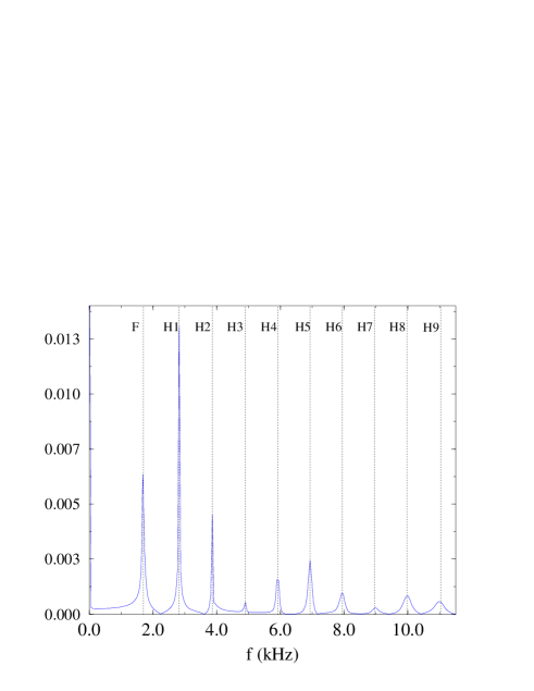
Figure 2: Fourier transform of the evolution of the radial velocity in Fig. 1. The frequencies are in excellent agreement with linear normal mode frequencies computed with an eigenvalue code. The units of the vertical axis are arbitrary.

To compare the obtained frequencies to linear normal mode frequencies, we use a different code that solves the linearized relativistic pulsation equations for the stellar fluid, in the Cowling approximation [31, 32, 33], as an eigenvalue problem. In Table 1 we present the results of this comparison. The typical agreement between frequencies computed by the two methods is better than 0.5% for the fundamental $F$-mode and the lowest frequency harmonics $H_{1}-H_{4}$ and better than 0.8% for the the higher harmonics $H_{5}-H_{9}$. This is a strong test for the accuracy of the evolution code and our results can be used as a testbed computation for other relativistic multi-dimensional evolution codes.

Radial Pulsation Frequencies
Mode	non-linear code (kHz)	Cowling (kHz)	difference
$F$	1.703	1.697	0.3%
$H_{1}$	2.820	2.807	0.5%
$H_{2}$	3.862	3.868	0.02%
$H_{3}$	4.900	4.910	0.2%
$H_{4}$	5.917	5.944	0.4%
$H_{5}$	6.930	6.973	0.6%
$H_{6}$	7.947	8.001	0.7%
$H_{7}$	8.960	9.029	0.8%
$H_{8}$	9.973	10.057	0.8%
$H_{9}$	11.030	11.086	0.5%

Table 1: Comparison of small-amplitude radial pulsation frequencies obtained with the present non-linear evolution code to linear perturbation mode frequencies in the relativistic Cowling approximation. The equilibrium model is a nonrotating $N=1.5$ relativistic polytrope with $M/R=0.056$.

Quadrupole Pulsation Frequencies
Mode	non-linear code (kHz)	Cowling (kHz)	difference
$f$	1.28	1.286	0.5%
$p_{1}$	2.68	2.681	0.04%
$p_{2}$	3.65	3.699	1.3%
$p_{3}$	4.66	4.719	1.3%
$p_{4}$	5.66	5.742	1.4%
$p_{5}$	6.83	6.764	1.0%
$p_{6}$	7.80	7.788	0.2%

Table 2: Comparison of small-amplitude quadrupole ($l=2$) pulsation frequencies obtained with the present non-linear evolution code to linear perturbation mode frequencies in the relativistic Cowling approximation. The equilibrium model is a nonrotating $N=1.5$ relativistic polytrope with $M/R=0.056$.

5.2 2-D evolutions

In a similar way, small-amplitude non-radial pulsations can be studied with the present evolution code and the obtained frequencies can be compared to perturbation results. We find that the truncation errors of the finite difference scheme do not excite non-radial pulsations to a sufficiently large amplitude compared to the amplitude of radial pulsations, so that one cannot identify them accurately in a Fourier transform. Instead, one has to perturb the initial configuration, using an appropriate eigenfunction for each nonradial angular index $l$. Such a perturbation can be constructed using the eigenfunctions of linear pulsation modes, computed with the perturbation code in the Cowling approximation. The frequencies of the non-radial modes are then found from a Fourier transform of the time-evolution of the velocity component $v_{\theta}$.

Table 2 shows a similar comparison as in Table 1 for the quadrupole ($l=2$) pulsations of the same $N=1.5$ relativistic polytrope. Since the non-radial modes have to be computed on a 2-D grid, we cannot use resolutions as high as in the 1-D computations. For a small grid-size of $80\times 80$ zones and a total evolution time of 6ms, the agreement between frequencies computed by the two methods is better than 1.4% for the fundamental $f$-mode and the $p$-modes $p_{1}-p_{6}$. For this grid-size, frequencies higher than the $p_{6}$ mode could not be computed accurately, because the grid is to coarse to resolve their eigenfunctions (higher harmonic eigenfunctions have a larger number of nodes in the radial direction).

6 Rotating Stars

We now turn to the evolution of initially stationary, uniformly rotating neutron stars. In these evolutions, we observe the same qualitative properties as for non-rotating stars (section 5) and an additional important property: the angular momentum of the star is not conserved at the surface layer. This is due to the fact that the velocity component $v_{\phi}$ of the fluid has a maximum at the surface, while the numerical scheme (although second-order accurate in smooth regions of the solution) is only first-order accurate at local extrema. Moreover, the code evolves the relativistic momenta, $S_{i}$, and the velocity components (as well as the rest of “primitive” variables) must be recovered through a root finding procedure which involves dividing by the density. At the surface of the star (where the density is very small) this contributes to obtaining less than second-order accuracy.

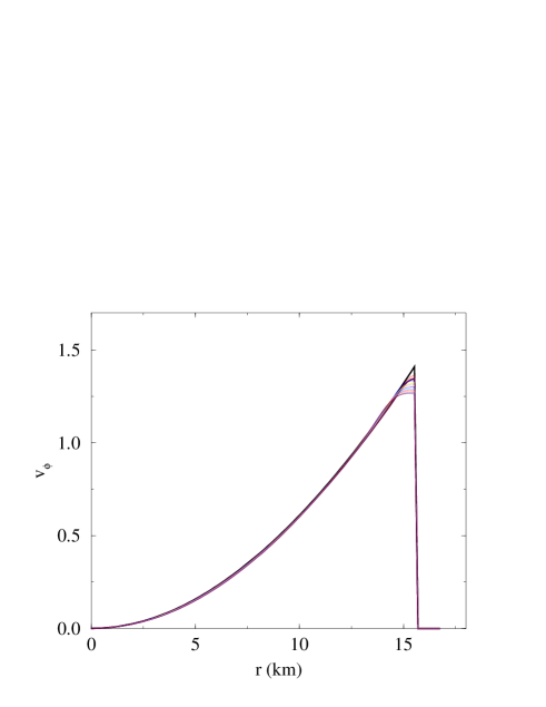
Figure 3: Time-evolution of the velocity component $v_{\phi}$ of a rotating star (see text for details). The accuracy is second order in the interior but only first order at the surface. This results in an angular momentum loss of the surface layers.

A representative example of the evolution of a rotating star is presented in Fig. 3, which shows the evolution, at different times, of the velocity component $v_{\phi}$. The star is again a $N=1.5$ polytrope with the same central density as the non-rotating star presented in section 5 and rotating at 74% of the mass-shedding limit at same central density. The evolution was for one rotation period on a $96\times 60$ grid. The vertical axis is dimensionless ($c=G=M_{\odot}=1$). The figure shows that the $\phi$-velocity in the interior of the star remains close to its initial value, while it decreases as a function of time in the outer layers. We find that this is a generic property of the present numerical scheme for any rotation rate and for any grid-size. By comparing evolutions with different grid sizes, we verified that the loss of angular momentum at the surface improves as first-order with resolution, while the evolution of the $\phi$-velocity in the interior is second-order accurate. However, as the evolution proceeds in time, the first-order surface effect gradually affects the interior of the star.

7 Quasi-radial Modes of Rotating Stars

As a first application of our code, we compute quasi-radial modes (i.e. modes that in the non-rotating limit reduce to radial modes) of rapidly rotating relativistic stars in the Cowling approximation. Previously, these modes have been computed for fully relativistic stars only in the slow-rotation limit (but without the assumption of a fixed spacetime) by Hartle & Friedman [34] (see also [35]). We compute the three lowest-frequency quasi-radial modes for a sequence of rotating stars of same central density. The non-rotating member of the sequence is the non-rotating star of section 5. Table 3 and Fig. 4 show our results for a low resolution grid of $100\times 80$ zones (note that our computational grid assumes equatorial plane symmetry). For this resolution we estimate the accuracy of the frequencies to be of the order of $1-2$%.

For the sequence of stars considered here, the frequencies of the quasi-radial modes decrease with increasing rotation rate. This agrees with previous slow-rotation computations which predict a decrease as $\Omega^{2}$, where $\Omega$ is the angular velocity of the star. For fast rotation, the change in the frequencies of quasi-radial modes is affected by higher order terms in $\Omega$, because of the large deformation of the equilibrium star. Also, for rapidly rotating stars the quasi-radial mode frequencies are more “closely packed” than in non-rotating stars.

Quasi-radial Pulsation Frequencies
$\Omega/\Omega_{K}$	F (kHz)	H1 (kHz)	H2 (kHz)
0.0	1.71	2.82	3.90
0.32	1.70	2.77	3.81
0.44	1.67	2.71	3.68
0.62	1.64	2.52	3.46
0.74	1.53	2.38	3.33
0.84	1.36	2.25	3.17

Table 3: Frequencies of quasi-radial modes for different values of the ratio of angular velocity of the star $\Omega$ to the angular velocity at the mass-shedding limit $\Omega_{K}$, for a sequence of rotating relativistic stars of same central density. The non-rotating member of the sequence is the same as in Table 1.

Figure 4: Frequencies of the lowest three quasi-radial modes vs. the ratio of angular velocity of the star $\Omega$ to the angular velocity at the mass-shedding limit $\Omega_{K}$, for the sequence of rotating relativistic stars in Table 3.

8 Discussion

Our axisymmetric relativistic hydrodynamical code is capable to evolve rapidly rotating stars in a fixed spacetime. We find that, for non-rotating stars, small amplitude oscillations have frequencies that agree with linear normal mode frequencies in the Cowling approximation and we compute the quasi-radial modes of rapidly rotating stars.

Modern HRSC numerical schemes (as the ones used in our code), satisfying the “total variation diminishing” (TVD) property [36], are second-order accurate in smooth regions of the flow, but only first-order accurate at local extrema. In our rotating stars runs we find that this results in a loss of angular momentum of the surface layers of the star, which gradually also affects the interior of the star. This angular momentum loss only vanishes as first-order with incresing resolution and we thus conclude that for accurate long-term evolutions of rotating neutron stars it is essential to use rather fine grids. Furthermore, to reduce the computational cost, one could use surface-adapted coordinates or fixed-mesh refinement. It would also be interesting to see whether the loss of angular momentum per rotation period will be significantly smaller in a frame co-rotating with the star. An alternative solution to this problem, which we plan to investigate, could be the use of “essentially non-oscillatory” (ENO) schemes, which maintain high-order of accuracy even at local extrema [37].

All previous considerations are important for the study of the non-linear dynamics of unstable toroidal oscillations ($r$-modes) in 3-D, which have a long growth time and thus require highly accurate long-term evolutions.

References

References

- [1] J.A. Font, M. Miller, W.-M. Suen, & M. Tobias, Phys. Rev. D, in press (1999) (gr-qc/9811015).
- [2] M. Shibata, T.W. Baumgarte & S.L. Shapiro, Phys. Rev. D. 58, 023002 (1998).
- [3] G.J. Mathews, P. Marronetti & J.R. Wilson, Phys. Rev. D. 58, 043003 (1998).
- [4] T. Nakamura & K. Oohara, talk at Numerical Astrophysics (1998) (gr-qc/9812054).
-
[5]
N. Stergioulas,
Living Reviews in Relativity, 1998-8 (1998)
(http://www.livingreviews.org/Articles/Volume1/1998-8stergio/). - [6] J.L. Houser, J.M. Centrella & S.C. Smith, Phys. Rev. Lett. 72, 1314 (1994).
- [7] S. Chandrasekhar, Phys. Rev. Lett. 24, 611 (1970).
- [8] J.L. Friedman & B.F. Schutz, ApJ 222, 281 (1978).
- [9] N. Andersson, Astrophys. J. 502, 708 (1998).
- [10] J.L. Friedman & S.M. Morsink, ApJ 502, 714 (1998).
- [11] N. Andersson, K.D. Kokkotas & B.F. Schutz, ApJ 510, 846 (1999).
- [12] L. Lindblom, B.J. Owen & S.M. Morsink, Phys. Rev. Lett. 80, 4843 (1998).
- [13] B.J. Owen, L. Lindblom, C. Cutler. B. F. Schutz, A. Vecchio & N. Andersson, Phys. Rev. D 58, 084020 (1998).
- [14] R. J. LeVeque, Numerical Methods for Conservation Laws (Birkhauser Verlag, Basel) (1992).
- [15] J.M. Ibáñez & J.M. Marti, J. Comput. Appl. Math., in press (1999).
- [16] J.V. Romero, J.M. Ibáñez, J.M. Marti & J.A. Miralles, ApJ 462, 836 (1996).
- [17] E. Gourgoulhon, Astr. Ap. 252, 651 (1991).
- [18] E. M. Butterworth & J.R. Ipser, ApJ 204, 200 (1976)
- [19] N. Stergioulas & J.L. Friedman, ApJ 444, 306 (1995).
- [20] H. Komatsu, Y. Eriguchi & I. Hachisu, MNRAS 237, 355 (1989).
- [21] G.B. Cook, S.L. Shapiro & S.A. Teukolsky, ApJ 398, 203 (1992).
- [22] T. Nozawa, N. Stergioulas, E. Gourgoulhon & Y. Eriguchi, Astr. Ap. Supp. Ser. 132, 431 (1998).
- [23] J.M. Marti, J.M. Ibáñez & J.A. Miralles, Phys. Rev. D 43, 3794 (1991).
- [24] F. Banyuls, J.A. Font, J.M. Ibáñez , J.M. Marti & J.A. Miralles, ApJ 476, 221 (1997).
- [25] P. Papadopoulos & J.A. Font, Phys. Rev. D, in press (1999) (gr-qc/9902018).
- [26] J.A. Font & P. Papadopoulos, these proceedings (1999).
- [27] J.A. Font, N. Stergioulas & K. Kokkotas, (in preparation) (1999).
- [28] P.L. Roe, J. Comput. Phys. 43, 357 (1981).
- [29] R. Donat & A. Marquina, J. Comput. Phys. 125, 42 (1996).
- [30] R. Donat, J.A. Font, J.M. Ibáñez & A. Marquina, J. Comput. Phys. 146, 58 (1998).
- [31] P.N. McDermott, H.M. Van Horn & J.F. Scholl, ApJ 268, 837 (1983).
- [32] L. Lindblom & R.J. Splinter, ApJ 348, 198 (1990).
- [33] S. Yoshida & Y. Eriguchi, ApJ, (in press) (1999) (astro-ph/9807254).
- [34] J.B. Hartle & J.L. Friedman, ApJ 196, 653 (1975).
- [35] B. Datta, S.S. Hasan, P.K. Sahu, A.R. Prasanna, International J. of Modern Physics D, Vol. 7, No. 1 49 (1998).
- [36] A. Harten, SIAM J. Numer. Anal. 21, 1 (1984).
- [37] A. Harten & S. Osher, SIAM J. Numer. Anal. 24, 279 (1987).