Numerical hydrodynamics on light cones

Abstract

Characteristic methods show excellent promise in the evolution of single black hole spacetimes. The effective coupling with matter fields may help the numerical exploration of important astrophysical systems such as neutron star black hole binaries. To this end we investigate formalisms for numerical relativistic hydrodynamics which can be adaptable to null (characteristic) foliations of the spacetime. The feasibility of the procedure is demonstrated with one-dimensional results on the evolution of self-gravitating matter accreting onto a dynamical black hole.

• Max-Planck-Institut für Gravitationsphysik, Albert-Einstein-Institut,
  Schlaatzweg 1, Potsdam, D-14473, Germany
  Email: font@aei-potsdam.mpg.de, philip@aei-potsdam.mpg.de

1 Introduction

The so-called characteristic formulation of the field equations of general relativity has proven recently to be well suited for numerical evolutions of single black hole (vacuum) spacetimes [1]. A three-dimensional characteristic code developed by the Binary Black Hole Grand Challenge Alliance in the US has achieved, for the first time, accurate and long-term stable evolutions of such spacetimes, including distorted, moving and spinning single black holes, with evolution times up to $60,000M$ [2]. Such evolutions are ultimately possible due to the excellent gauge control properties furnished by null foliations, gauge control being a major open issue in the more usual 3+1 formulation.

The incorporation of matter terms into such a computational framework, in the form of some suitable stress-energy tensor, permits the study of interesting astrophysical scenarios with optimal computational efficiency. Such an approach allows to investigate the non-linear evolution of self-gravitating matter around dynamic black holes. Some interesting astrophysical studies to be performed include, e.g., accretion disks or the non-linear and fully relativistic evolution of a compact binary system formed by a black hole and a neutron star. This binary system is one of the anticipated sources of gravitational radiation. Its detailed numerical study can provide valuable information on the waveform signals and a means to decipher the nuclear equation of state.

In this report we focus on the formulation of the hydrodynamic equations on null foliations of the spacetime. The reader must be aware that most of the previous analytic and numerical work in general relativistic hydrodynamics (GRH hereafter) has been done using the “standard” 3+1 formulation, i.e., using a spacetime foliation of spacelike hypersurfaces (see, e.g., [3] and references therein). Additionally, the small amount of existing work dealing with the numerical integration of the GRH equations on null hypersurfaces can be characterized by: a) a direct way of writing the hydrodynamic equations with no attention to important mathematical (and numerical) details (as, e.g., hyperbolicity) and b) the use of straightforward finite-differences numerical schemes [4],[5],[6]. However, on the basis of the experience gained in the last few years in the integration of the hydrodynamic equations in the spacelike case, we believe that the procedure previously adopted for the null case is likely to be inadequate when dealing with non-trivial simulations. Most notably we refer to realistic astrophysical scenarios containing high speed (ultrarelativistic) flows and steep gradients or even shock waves.

As a way to avoid these problems we propose the use of the so-called high-resolution shock-capturing schemes (HRSC in the following) to integrate the GRH equations on light cones. HRSC schemes are commonly used in numerical integrations of the Newtonian inviscid Euler equations. In recent years they have been succesfully extended to relativistic hydrodynamics, both in the special and general cases [7],[8],[9],[3],[10]. Mathematically, HRSC schemes rely on the hyperbolic character of the hydrodynamic equations. The knowledge of the characteristic fields (eigenvalues) of the system, together with the corresponding eigenvectors, allows for accurate integrations, by means of either exact or approximate Riemann solvers, along the fluid characteristics.

Among the interesting properties of HRSC schemes we stress the important fact that they are written in conservation form. Hence, all physically conserved quantities of a given partial differential equation will also be conserved in its finite-differenced version. More precisely, the time update of the following hyperbolic one-dimensional partial differential system of equations

$$\frac{\partial{\bf u}}{\partial t}+\frac{\partial{\bf f}}{\partial x}={\bf s}$$ (1)

is done according to the following algorithm:

$${\bf u}_{i}^{n+1}={\bf u}_{i}^{n}-\frac{\Delta t}{\Delta x}(\widehat{{\bf f}}_{i+1/2}-\widehat{{\bf f}}_{i-1/2})+\Delta t{\bf s}_{i}.$$ (2)

In these expressions ${\bf f}$ and ${\bf s}$ are vector-valued functions, the fluxes and sources, and they both depend on the state vector of the system ${\bf u}$. Index $i$ labels the grid location and $n$ the time. Time and space discretization intervals are indicated by $\Delta t$ and $\Delta x$, respectively. The “hat” in the fluxes is used to denote the so-called numerical fluxes which, in a HRSC scheme, are computed according to some generic flux-formula. It adopts the following functional form:

$$\widehat{{\bf f}}_{i\pm{1\over 2}}=\frac{1}{2}\left({\bf f}({\bf u}_{i\pm{1\over 2}}^{L})+{\bf f}({\bf u}_{i\pm{1\over 2}}^{R})-\sum_{\alpha=1}^{p}\mid\widetilde{\lambda}_{\alpha}\mid\Delta\widetilde{\omega}_{\alpha}\widetilde{r}_{\alpha}\right).$$ (3)

Notice that the numerical flux is computed at cell interfaces ($i\pm 1/2$). Indices $L$ and $R$ indicate the left and right sides of a given interface. The sum extends to $p$, the total number of equations. Finally, quantities $\lambda$, $\Delta\omega$ and $r$ denote the eigenvalues, the jump of the characteristic variables and the eigenvectors, respectively, computed at the cell interfaces according to some suitable average of the state vector variables. Further technical information can be found in, e.g. [8] and references therein.

HRSC schemes are also known for giving stable and sharp discrete shock profiles. They have also a high order of accuracy, typically second order or more, in smooth parts of the solution.

2 A covariant form of the general relativistic hydrodynamic equations

The conservation equations in covariant form are

$$\frac{\partial}{\partial x^{\mu}}\sqrt{-g}J^{\mu} = 0$$ (4)

$$\frac{\partial}{\partial x^{\mu}}\sqrt{-g}T^{\mu\nu} = -\sqrt{-g}\Gamma^{\nu}_{\mu\lambda}T^{\mu\lambda}$$ (5)

with the matter current and stress energy tensor for a perfect fluid given by $J^{\mu}=\rho u^{\mu}$, $T^{\mu\nu}=\rho hu^{\mu}u^{\nu}+pg^{\mu\nu}$, where $\rho$ is the density, $p$ the pressure and $u^{\mu}$ the fluid four velocity obeying the normalization condition $u_{\mu}u^{\mu}=-1$. Additionally, $h=1+\epsilon+p/\rho$ is the relativistic specific enthalpy, with $\epsilon$ being the specific internal energy.

The construction of an initial value problem requires the introduction of a coordinate chart $(x^{0},x^{i})$, where the scalar $x^{0}$ represents a foliation of the spacetime with hypersurfaces (coordinatized by $(x^{1},x^{2},x^{3})$) on which an appropriate initial data set is prescribed. Upon introducing the coordinate chart, we define the coordinate components of the four-velocity $u^{\mu}=(u^{0},u^{i})$. The velocity components $u^{i}$, together with the rest-frame density and internal energy, $\rho$ and $\epsilon$, provide a unique description of the state of the fluid and are called the primitive variables. They consitute a vector in a five dimensional space ${\bf w}^{A}=(\rho,u^{i},\epsilon)$. The index A is taken to run from zero to four, coinciding for the values (1,2,3) with the coordinate index $i$.

We define the initial value problem in terms of another vector in the same fluid state space, namely the conserved variables ${\bf U}^{B}$, individually denoted $(D,S^{i},E)$, as follows:

$$D = {\bf U}^{0}=J^{0}=\rho u^{0}$$ (6)

$$S^{i} = {\bf U}^{i}=T^{0i}=\rho hu^{0}u^{i}+pg^{0i}$$ (7)

$$E = {\bf U}^{4}=T^{0t}=\rho hu^{0}u^{0}+pg^{00}$$ (8)

With these definitions the equations take the standard conservation law form

$$\partial_{x^{0}}(\sqrt{-g}{\bf U}^{A})+\partial_{x^{j}}(\sqrt{-g}{\bf F}^{jA})={\bf S}^{A}$$ (9)

where ${\bf S}^{A}({\bf w}^{B})$ are source terms that depend on metric derivatives and the (undifferentiated) stress energy tensor, $\sqrt{-g}$ is the volume element associated with the four-metric and we define the flux vectors ${\bf F}^{jA}$

$${\bf F}^{j0} = J^{j}=\rho u^{j}$$ (10)

$${\bf F}^{ji} = T^{ji}=\rho hu^{i}u^{j}+pg^{ij}$$ (11)

$${\bf F}^{j4} = T^{j0}=\rho hu^{0}u^{j}+pg^{0j}$$ (12)

The source terms take the form

$${\bf S}^{0} = 0$$ (13)

$${\bf S}^{i} = -\sqrt{-g}\,\Gamma^{i}_{\mu\lambda}T^{\mu\lambda}$$ (14)

$${\bf S}^{4} = -\sqrt{-g}\,\Gamma^{0}_{\mu\lambda}T^{\mu\lambda}$$ (15)

For a complete description of the local characteristic structure of the previous equations, which is the basic ingredient to make use of HRSC schemes, we refer the interested reader to [12]. We end this section by stressing that the previous formulation of the GRH equations is fully covariant and, hence, both applicable to spacelike or null spacetime foliations. The results we show next are specialized to null foliations.

3 Results

3.1 The Riemann problem on a null surface

This section is devoted to demonstrate the functionality of our approach in a standard hydrodynamical testbed computation, the Riemann problem. This is one of the standard tests to calibrate numerical schemes in fluid dynamics. It provides a strong check of our procedure in the limiting case of Minkowski spacetime. Initial data are given on the light cone and the evolution is compared to the exact solution. The initial setup consists of a zero velocity fluid having two different thermodynamical states on either side of an interface. In our setup the initial state is specified by $p_{r}=13.3$, $\rho_{r}=10$ at the right side of the interface and $p_{l}=0.66\cdot 10^{-6}$, $\rho_{l}=1$ at the left side. We use a perfect fluid equation of state, $p=(\Gamma-1)\rho\epsilon$ with $\Gamma=5/3$. When the interface is removed, the fluid evolves in such a way that four constant states occur. Each state is separated by one of three elementary waves: a shock wave, a contact discontinuity and a rarefaction wave.

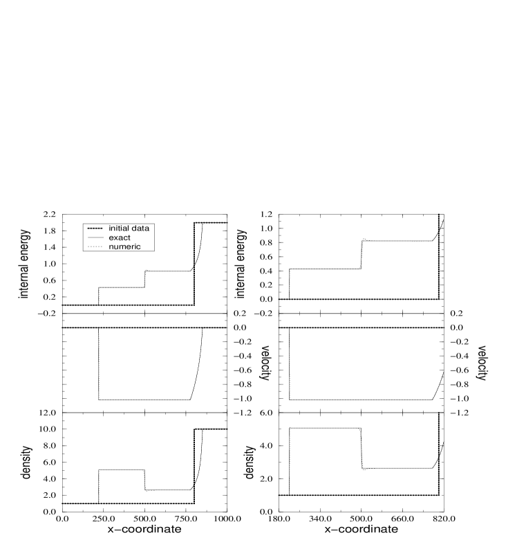
Figure 1: The shock tube problem. Exact versus numerical solution at a retarded time $v=120$ for the internal energy (top), velocity (middle) and density (bottom).

In Fig. 1 we plot the results of the simulation. The left pannels show the whole domain, with the $x$-coordinate ranging from 0 to 1000 whereas the right pannels show a closed-up view of the most interesting region ($x\in[180,820]$). We use a numerical grid of 2000 zones and, hence, a rather coarse spatial resolution ($\Delta x=0.5$). The initial data are evolved up to a final time $v=120$. From top to bottom Fig. 1 displays the internal energy ($\epsilon$), the velocity ($u^{x}$) and the density ($\rho$). The thick dotted line represents the initial discontinuity. The solid line shows the exact solution after a retarded time $v=120$ and the thin dotted line indicates the numerical solution at this same time. The agreement between the two solutions is remarkable. The flow solution is characterized by an (ingoing) shock wave (moving to the left) and an (outgoing) rarefaction wave (moving to the right). We note that those features of the solution moving towards the left are more developed than those moving towards the right. The major numerical deviations from the exact solution appear at the post contact discontinuity region, with the density and the internal energy being slightly under and over estimated there.

3.2 Spherical accretion onto a black hole

We further test our procedure by increasing the complexity of the numerical simulation with the inclusion of gravity. To this end, we consider the problem of spherical accretion of a perfect fluid onto a black hole.

We consider the general spherically symmetric spacetime with perfect fluid matter, following the formalism of Tamburino-Winicour [13]. The use of a spacetime foliation $v$ by null hypersurfaces ($\nabla^{\mu}v\nabla_{\mu}v=0$), together with the assumption of spherical symmetry implies that the non-trivial Einstein equations split in the following group of equations

$$G_{vr} = \kappa T_{vr},$$ (16)

$$G_{rr} = \kappa T_{rr},$$ (17)

$$G_{vv}|_{\Gamma} = \kappa T_{vv}|_{\Gamma},$$ (18)

where the last equation is a conservation condition to be imposed on the boundary $\Gamma$ of the integration domain. Adopting the Bondi-Sachs form of the metric element,

$$ds^{2}=-\frac{e^{2\beta}V}{r}dv^{2}+2e^{2\beta}dvdr+r^{2}(d\theta^{2}+\sin\theta^{2}d\phi^{2}),$$ (19)

the geometry is completely described by the functions $\beta(v,r)$ and $V(v,r)$.

The first two equations above, Eqs. (16) and (17), are hypersurface equations, to be integrated away from $\Gamma$ along the null cone. The $\beta$ hypersurface equation is

$$\beta_{,r}=2\pi rT_{rr}$$ (20)

and the $V$ hypersurface equation,

$$V_{,r}=e^{2\beta}(1-4\pi r^{2}(g^{AB}T_{AB}-T)).$$ (21)

Boundary conditions $\beta(v)_{\Gamma},V(v)_{\Gamma}$ for the radial integrations are provided by the third equation, after adopting a suitable gauge condition. This condition fixes the only remaining freedom in the coordinate system, namely the rate of flow of coordinate time at the world-tube. We refer the reader to [12] for a discussion on suitable gauge conditions.

The initial data consist of the fluid variables $(\rho,\epsilon,u^{r})$ on the initial slice $v_{0}$, together with the values of $\beta(v_{0})_{\Gamma}$ and $V(v_{0})_{\Gamma}$.

In the limit of a test fluid, i.e., a perfect fluid with sufficiently low density accreting spherically onto a static black hole, the numerical evolution can be compared to an exact solution. This comparison was performed and the agreement was found to be excellent. We refer the interested reader to [12] (see also [11]) for further information. We focus here on the case of spherical accretion onto a dynamic black hole.

Figure 2: Spherical accretion of a self-gravitating perfect fluid: evolution of the Riemann scalar curvature. Once the shell is swallowed by the central object the solution is dominated by the curvature of the final black hole.

As initial data we consider the exact, stationary solution corresponding to the test fluid case and, on top of this background solution, we build a self-gravitating spherically symmetric shell whose density is parametrized by a Gaussian profile with suitable width and amplitude. The results of the simulation are plotted in Figs. 2 and 3. We find that the shell is radially advected (accreted) towards the hole in the first $10M-15M$. Once the bulk of the accretion process ends, we are left with a quasi-stationary background solution. This is clear in Fig. 2, where we plot the evolution of the logarithm of the Riemann scalar curvature, as a function of the ingoing Eddington-Finkelstein radial coordinate, $r$. This variable encodes a large amount of relevant metric information. We note that the initial shell has a non-negligible curvature. After the shell is accreted by the hole the curvature profile monotonically increases towards the central singularity. The accretion of the shell originates a rapid increase on the mass of the apparent horizon of the black hole. This is depicted in Fig. 3. The horizon almost doubles its size during the first $10M-15M$ (this is enlarged in the insert of Fig. 3). Once the main accretion process has finished, the mass of the horizon slowly increases, in a quasi-steady manner, whose rate depends on the mass accretion rate imposed at the world-tube, $\Gamma$, of the integration domain. We emphasize the fact that this numerical solution can be evolved as far as desired into the future. It has proven to remain remarkably stable and free of any kind of numerical pathologies, including secular instabilities or exponentially growing modes.

Figure 3: Spherical accretion of a self-gravitating perfect fluid: evolution of the black hole apparent horizon mass.

References

References

- [1] N. Bishop, R. Gómez, L. Lehner, M. Maharaj, & J. Winicour, Phys. Rev. D 56, 6298 (1997).
- [2] R. Gómez, et al., Phys. Rev. Lett. 80, 3915 (1998).
- [3] F. Banyuls, J.A. Font, J.M. Ibáñez, J.M. Marti, & J.A. Miralles, ApJ 476, 221 (1997).
- [4] R.A. Isaacson, J.S. Welling, & J. Winicour, J. Math. Phys. 24, 1824 (1983).
- [5] M. Dubal, R. d’Inverno, & J.A. Vickers, Phys. Rev. D 58, 4019 (1998).
- [6] N. Bishop, R. Gómez, L. Lehner, M. Maharaj, & J. Winicour, Phys. Rev. D, submitted (1998).
- [7] J.M. Marti, J.M. Ibáñez, & J.A. Miralles, Phys. Rev. D 43, 3794 (1991).
- [8] J.A. Font, J.M. Ibáñez, A. Marquina, & J.M. Marti, Astr. Ap. 282, 304 (1994).
- [9] F. Eulderink, & G. Mellema, Astr. Ap. Suppl. Ser. 110, 587 (1995).
- [10] J.A. Font, M. Miller, W.-M. Suen, & M. Tobias, Phys. Rev. D, in press (1998).
- [11] P. Papadopoulos, & J.A. Font, Phys. Rev. D 58, 024005 (1998).
- [12] P. Papadopoulos, & J.A. Font, Phys. Rev. D, in press (1999).
- [13] L.A. Tamburino, & J. Winicour, Phys. Rev. 150 4, 1039 (1966).