Gravitational radiation sources and signatures

1 Introduction

The goal of these lecture notes is to introduce the developing research area of gravitational-wave phenomenology. In more concrete terms, they are meant to provide an overview of gravitational-wave sources and an introduction to the interpretation of real gravitational wave detector data. They are, of course, limited in both regards. Either topic could be the subject of one or more books, and certainly more than the few lectures possible in a summer school. Nevertheless, it is possible to talk about the problems of data analysis and give something of their flavor, and do the same for gravitational wave sources that might be observed in the upcoming generation of sensitive detectors. These notes are an attempt to do just that.

Despite an 83 year history, our best theory explaining the workings of gravity — Einstein’s theory of general relativity — is relatively untested compared to other physical theories. This owes principally to the fundamental weakness of the gravitational force: the precision measurements required to test the theory were not possible when Einstein first described it, or for many years thereafter.

The direct detection of gravitational-waves is a central component of our first investigations into the dynamics of the weakest of the known fundamental forces: gravity. It is only in the last 35 years that general relativity has been put to significant test. Today, the first effects of static relativistic gravity beyond those described by Newton have been well-studied using precision measurements of the motion of the planets, their satellites and the principal asteroids. Dynamical gravity has also been tested through detailed and comprehensive observations of the slow, secular decay of the Hulse-Taylor binary pulsar system [1, 2]. What has not heretofore been possible is the direct observation of the effects of dynamical gravity on a laboratory instrument: i.e., the direct detection of gravitational radiation.

The scientific importance of the direct detection of gravitational-waves does not stop with its detection, however. Strong gravitational-waves are difficult to generate: so difficult, in fact, that there is no possibility of a gravitational-wave “Hertz”-type experiment, where both the source and receiver are under laboratory control. The strongest gravitational-waves incident on Earth, as measured by our ability to detect them in the sensitive detectors now under construction, arise from astronomical sources. These are also the only sources that we can hope to observe in our detectors. The strongest of these anticipated sources — inspiraling or colliding neutron stars or black holes — are, in fact, of cosmological origin.

Very little relevant detail is known about the gravitational-wave sources that we anticipate may be detectable in the instruments now under construction. Estimates of source strengths and event rates are difficult to make reliably. This is because, at a deep and fundamental level, our understanding of the cosmos is limited to what we can learn from photons. The mechanism by which gravitational-waves are generated, on the other hand, favors sources that either do not radiate electromagnetically (e.g., black holes), are obscured from view (e.g., the gravitational collapse of a stellar core), or are so distant and decoupled from the immediate origin of the corresponding electromagnetic radiation that we cannot reliably decipher the relevant source characteristics from the photons that reach us (e.g., $\gamma$-ray bursts).[3]

Gravitational-wave observations thus add a new dimension to our ability to observe the Universe: the observations that we make will tell us things we don’t already know through other means.

In order to describe sensibly the signature of gravitational-wave sources in real detectors we must first discuss in some detail how we characterize gravitational-waves, how we characterize gravitational-wave detectors, and how we give operational meaning to the word “detect”. These three subjects are addressed in sections §2, §3 and §4, respectively. In the context of gravitational-wave detection, gravitational-wave signals fall fairly neatly into three categories: burst signals, periodic signals and stochastic signals. Sources thought to be responsible for detectable signals in these categories are described in sections §5.1, §5.2 and §5.3, respectively.

1.1 Conventions

• The distance from detector to source will always be large compared to either a wavelength of the radiation field or the physical dimension of the detector; consequently, the incident radiation is effectively planar.

• We choose a sign convention for the line element of Minkowskii spacetime and recall the Einstein summation convention, wherein repeated Greek indices in a product are implicitly summed over their full range:

  $$ds^{2} = \eta_{\mu\nu}\,dx^{\mu}\,dx^{\nu}$$ (1)

  $$= \sum_{\mu,\nu=0}^{3}\eta_{\mu\nu}\,dx^{\mu}\,dx^{\nu}$$ (2)

  $$= -c^{2}\left(dx^{0}\right)^{2}+\left(dx^{1}\right)^{2}+\left(dx^{2}\right)^{2}+\left(dx^{3}\right)^{2}$$ (3)

  $$= -c^{2}dt^{2}+dx^{2}+dy^{2}+dz^{2}.$$ (4)

• We will always treat the gravitational fields as weak and use coordinates on spacetime that are either “Cartesian”$+$time or “spherical-polar”$+$time.

• We will find it convenient to introduce the use of Latin indices to represent just the spatial components (i.e., $x$, $y$, and $z$) of a tenser. We generalize the Einstein summation convention to apply to repeated Latin indices in a product expression, with the implicit sum running over just the spatial coordinates, e.g.,

  $$x^{i}y_{i}=\sum_{j=1}^{3}x^{j}y_{j}.$$ (5)

• Except in the first several sections of these lecture notes, we will always work in units where the Newtonian gravitational constant $G$ and the speed of light $c$ are numerically equal to unity and the appearance of these constants in various formulae will be suppressed. Dimensional analysis will always suffice to determine how the formulae should appear with the constants in place.

• Using $c$ we can express time in units of length and frequency in units of inverse length; similarly, by exploiting $G$ and $c$ we can express mass and energy in units of length. Power is then a dimensionless number. For CGS units, the conversion factors between mass, energy and length, and the physical constant with units of power, are

  $$G/c^{2} = 7.42\times 10^{-29}\,\mbox{cm/gm}$$ (6)

  $$G/c^{4} = 8.26\times 10^{-50}\,\mbox{cm/erg}$$ (7)

  $$c^{5}/G = 3.63\times 10^{59}\,\mbox{erg/s}.$$ (8)

2 Characterizing Gravitational Radiation

For our purpose here — recognizing gravitational waves incident on a detector — two different characterizations of gravitational radiation are useful. The first is the radiation waveform and the second is the signal “power spectrum”. The waveform describes the radiation field’s time dependence while the power spectrum describes its Fourier components. In §2.1 and §2.3 we describe these different characterizations of gravitational radiation. Several important physical insights regarding gravitational radiation sources can be gained by considering the instantaneous power radiated by a source: we discuss these insights in §2.2.

2.1 Radiation waveform

In this subsection we review briefly the expression of the radiation incident on a detector. Much of this section is by way of review; for more details, see either the lectures by Bob Wagoner in this collection, one of the many text books on relativity[4, 5, 6, 7, 8], or an excellent review article on the subject.[9]

Gravitation manifests itself as spacetime curvature and gravitational waves as ripples in the curvature that appear to us, moving through time, to be propagating. Detectors are generally not directly sensitive to curvature, but to the mechanical displacement of their components; so, we focus our attention on the spacetime metric, from which physical distances between points in spacetime are determined. (The curvature is a function of the metric’s second derivatives.)

We assume that gravity is weak in and around our detector; correspondingly, we treat the spacetime metric as if it were the metric of Minkowskii spacetime, plus a small perturbation:

$$g_{\mu\nu}=\eta_{\mu\nu}+h_{\mu\nu},$$ (9)

where $\eta_{\mu\nu}$ is the Minkowskii metric and $h_{\mu\nu}$ the metric perturbation. The corresponding line element, describing the proper distance between nearby spacetime events whose coordinate separation is the infinitesimal $dx^{\mu}$, is

$$ds^{2}=g_{\mu\nu}dx^{\mu}dx^{\nu}=\eta_{\mu\nu}dx^{\mu}dx^{\nu}+h_{\mu\nu}dx^{\mu}dx^{\nu}.$$ (10)

Detecting gravitational waves amounts to building instruments that are sensitive to the effects of the small perturbation $h_{\mu\nu}$; determining the signature of the gravitational waves in the detector thus requires determining $h_{\mu\nu}$ and its influence on the detector.

The metric $g_{\mu\nu}$ tells us how the proper distance between points in spacetime is associated with our choice of coordinate system. Since the gravitational fields near our detector are weak and the spacetime nearly Minkowskii, we can introduce coordinates that are, in the neighborhood of the detector, nearly the usual Minkowskii-Cartesian coordinates, with the deviations of the order of the perturbation.

Now, small changes in the coordinate system do not change the proper distance between events, only our labeling of them. If we make small changes in our coordinate system, of the order of the perturbation, then we will make corresponding changes in the perturbation $h_{\mu\nu}$. We can use this freedom to simplify the expression of $h_{\mu\nu}$. Coordinate changes do not change the physics or any observable constructed from $h_{\mu\nu}$, of course. For this reason, and in analogy with electromagnetism, coordinate choices like these are referred to as gauge choices.

With the separation of the metric into the Minkowskii metric $\eta_{\mu\nu}$ plus a small perturbation, the field equations of general relativity become (at first order in the perturbation) a set of second order, linear differential equations for the ten components of the symmetric $h_{\mu\nu}$. Consequently, fixing the coordinates allows us to impose eight conditions on the ten components of the symmetric $h_{\mu\nu}$, leaving just two dynamical degrees of freedom. These are identified as the two polarizations of the gravitational radiation field.

An important gauge choice, always possible for radiative perturbations about Minkowskii space, is the Transverse-Traceless, or TT, gauge. Transverse-Traceless gauge is always associated with a particular observer of the radiation. Let the four-velocity of this observer have components $U^{\mu}$. Without loss of generality let $t$ mark the proper-time of this observer (so that $U^{\mu}$ is just the coordinate vector in the $t$ direction) and $x$, $y$ and $z$ be the usual Cartesian coordinates (to ${\cal O}(h)$) in the neighborhood of the observer. In TT-gauge the field equations are

$$\left(-{\partial^{2}\over\partial t^{2}}+\nabla^{2}\right)h_{\mu\nu}=-16\pi T_{\mu\nu},$$ (11)

subject to the constraints

$$h_{\mu\nu}U^{\mu} = 0,$$ (12)

$${\partial\over\partial x^{k}}\left(h_{j\mu}\eta^{\mu k}\right) = h_{j}{}^{k}{}_{,k}=0,$$ (13)

$$h_{jk}\delta^{jk} = 0;$$ (14)

The metric perturbation satisfies a wave equation whose source is the stress-energy density $T_{\mu\nu}$ of the matter and (non-gravitational) fields. In more physical terms, the constraints are (in order):

• $h_{\mu\nu}$ is purely spatial;

• the (spatial) metric perturbation $h_{ij}$ is purely transverse: i.e., if the radiation wavevector is $k^{i}$ (where the index $i$ runs over just the spatial dimensions; see §1.1), then $h_{ij}k^{i}$ vanishes for all $j$; and

• the metric perturbation is trace-free.

When there might be confusion we denote a metric perturbation in TT-gauge with a superscript TT on $h_{\mu\nu}$; also, since the perturbation is purely spatial, we generally refer just to the spatial projection (in the coordinate system of the observer) of the perturbation, as in $h^{TT}_{ij}$.

Given a metric perturbation $h^{\prime}_{\mu\nu}$, expressed in any gauge, corresponding to a plane wave propagating in the direction $n^{k}$, we can recover the corresponding metric perturbation in TT-gauge by applying the linear operator $P_{lm}$ to the spatial $h^{\prime}_{ij}$:

$$h^{TT}_{ij} = P_{i}^{l}h^{\prime}_{lm}P^{m}_{j}-{1\over 2}P_{ij}P^{lm}h^{\prime}_{lm}$$ (15)

$$P_{lm} = \delta_{lm}-n_{l}n_{m}.$$ (16)

Here and henceforth we will always express the metric perturbation in TT-gauge.

As mentioned above, gravitational wave detectors work by sensing the relative motion of their components induced by a passing gravitational wave. Let’s see how the TT-gauge metric perturbation is related to such relative motion.

Consider a single isolated test mass, initially at rest at coordinate position $\vec{x}_{A}$ in a TT-gauge coordinate system. No forces act on this test mass; so, it moves through spacetime in such a way that its four-velocity always remains tangent to itself. (Forces, of course, cause the four-velocity to change direction.) The corresponding equations of motion for the spatial coordinates of the test mass are

$${d\over d\tau}\left(dx^{i}_{A}\over d\tau\right)+\Gamma^{i}_{\mu\nu}{dx^{\mu}_{A}\over d\tau}{dx^{\nu}_{A}\over d\tau}=0,$$ (17)

where $\tau$ is the proper time of the test mass (initially $\tau$ is equal to $t$ since the test mass is at rest) and $\Gamma^{\alpha}_{\beta\gamma}$ is the metric connection

$$\Gamma^{\alpha}_{\beta\gamma}={1\over 2}g^{\alpha\mu}\left(g_{\mu\beta,\gamma}+g_{\mu\gamma,\beta}-g_{\gamma\beta,\mu}\right).$$ (18)

(Recall that _,k represents the derivative $\partial/\partial x^{k}$.) Since the test mass is initially at coordinate rest the $dx^{i}/d\tau$ vanish initially; so, the only connection component of interest is $\Gamma^{i}_{tt}$. In TT-gauge, however, this component of the connection is identically zero (recall that $h^{TT}_{\mu\nu}$ is purely spatial); so, the equations of motion reduce to

$${d\over d\tau}{dx^{i}_{A}\over d\tau}=0;$$ (19)

i.e., a free test particle at (TT-gauge) coordinate rest remains at coordinate rest. This applies equally well for a second component of the detector, located at $\vec{x}_{B}$: it, too, remains at coordinate rest.

This may seem paradoxical: if the coordinate separation of any two components of a detector remain unchanged by the passage of a gravitational wave, what is there to show the wave’s existence? The paradox vanishes when we realize that coordinate separation is not physical separation. To determine the physical separation of the detector’s components we must invoke the metric again. Let the coordinate separation between the two components of the detector at time $t$ be the infinitesimal $dx^{i}_{AB}$,

$$dx^{i}_{AB}=x_{B}^{i}-x_{A}^{i}.$$ (20)

(Of course, $dt=0$ since we are talking about separation at the same coordinate time.) The physical distance between these two neighboring points in spacetime is

$$ds^{2} = g_{\mu\nu}dx^{\mu}dx^{\nu}$$ (21)

$$= \eta_{\mu\nu}dx^{\mu}_{AB}dx^{\nu}_{AB}+h^{TT}_{\mu\nu}dx_{AB}^{\mu}dx_{AB}^{\nu}$$ (22)

$$= \eta_{jk}dx^{j}_{AB}dx^{k}_{AB}+h^{TT}_{jk}dx^{j}_{AB}dx^{k}_{AB}.$$ (23)

The second term in equation 23 shows the effect of the gravitational wave on the separation between the two elements of the detector: as $h_{\mu\nu}$ oscillates, so does the distance. If the equilibrium separation between the components is $L$ in the direction $\hat{n}^{j}$, to ${\cal O}(h)$ the net change $\delta L$ in the separation is equal to

$$\delta L={1\over 2}Lh^{TT}_{jk}\hat{n}^{j}\hat{n}^{k}.$$ (24)

The physical distance between detector components does change, in an amount proportional to the undisturbed separation and the wave strength as projected on the separation. Gravitational wave detectors are designed to be sensitive to this displacement of their components.

As mentioned above, the TT-gauge conditions amount to eight constraints on the ten otherwise independent components of the (symmetric) $h_{\mu\nu}$. There are thus two components of $h_{\mu\nu}$ that are independent of the choice of coordinate system; correspondingly, in general relativity there are two dynamical degrees of freedom of the gravitational field. To see what what these amount to, without loss of generality consider a plane wave propagating in the $z$ direction. Then we can write

$$h:^{TT}_{\mu\nu}dx^{\mu}dx^{\nu}=h_{+}(x^{i},t)\left(dx^{2}-dy^{2}\right)+2h_{\times}(x^{j},t)dx\,dy,$$ (25)

where $h_{+}$ and $h_{\times}$ are the two independent dynamical degrees of freedom, or polarizations, of the gravitational radiation field.

Solutions to the wave equation for $h_{ij}$ (eq. 11) can be analyzed in a slow motion expansion in exactly the same way as solutions to the Maxwell equations.[10, 9, 11] The radiative $h_{ij}$ in this expansion divide neatly into two classes of multipolar fields, which are (in analogy with electromagnetism) termed electric and magnetic multipoles. The electric multipolar radiative fields are generated by time-varying multipole moments of the source matter density in the same way that the analogous electric moments of the Maxwell field are generated by the time-varying moments of the electric charge density. Similarly, the magnetic radiative moments are generated by the time-varying multipole moments of the matter momentum density, which is the analog of the electric current density.

In electromagnetism, the first radiative moment of a charge distribution is a time-varying charge dipole moment. When electrical charge is replaced by gravitational charge — i.e., mass — we see that the corresponding dipole is just the position of the system’s center of mass, which (owing to momentum conservation) is unaccelerated. Consequently, in general relativity there is no gravitational dipole radiation. The first gravitationally radiative moment of a matter distribution arises from its “accelerating” quadrupole moment. Dotting the i’s and crossing the t’s, we find that, at leading order, the radiation field at a distant detector is related to the matter distribution of the source according to

$$h^{TT}_{ij}(t,\vec{x}) = {2\over r}{G\over c^{5}}{d^{2}\over dt^{2}}{Q}_{ij}^{TT}(t-r)$$ (26)

$$Q_{ij}^{TT} = P_{ik}(\vec{x})Q_{kl}P_{lj}(\vec{x})-{1\over 2}P_{ij}(\vec{x})Q_{lm}P_{lm}(\vec{x})$$ (27)

$$Q_{ij}(t) = \int d^{3}x\,\rho(t,\vec{x})\left(x_{i}x_{j}-{1\over 3}\delta_{ij}\right),$$ (28)

$$P_{jk}(\vec{x}) = \delta_{jk}-x_{j}x_{k}/x^{2}.$$ (29)

The expression for $h^{TT}_{ij}$ given above is the famous “quadrupole formula” of general relativity, which relates the acceleration of a source’s quadrupole moment to the gravitational radiation emitted. It is, for weak gravitational fields, the exact analog of the more famous “dipole formula” of electromagnetism.

2.2 Radiated power or energy

Gravitational radiation carries energy away from the radiating system. Important insights into gravitational radiation can be gained by considering the energetics of radiation sources, which we do in this section.

The instantaneous power carried by the radiation is, in the usual way, proportional to the square of the time derivative of the field integrated over a sphere surrounding the source:

$$L\propto{c^{5}\over G}4\pi r^{2}\dot{h}^{2}.$$ (30)

The “exact” expression for the power carried away in electric quadrupole radiation is

$$L={1\over 5}{G\over c^{5}}\left<{d^{3}Q_{ij}\over dt^{3}}{d^{3}Q^{ij}\over dt^{3}}\right>,$$ (31)

where the $<>$ indicates an average several periods of the radiation. Note that the power depends on $Q_{ij}$ and not $Q^{TT}_{ij}$.

If we focus on the radiation emitted by a weak-field, dynamical source, we can use the multipolar expansions described above to replace the fields by the multipole moments of the source. For an electric $\ell$-pole field radiated by a matter source with mass $M$, typical dimension $R$ and internal velocity $V$,

$$L^{(\ell)}_{\mbox{electric}}\propto{c^{5}\over G}\left[{GM\over c^{2}R}\left({V\over c}\right)^{\ell+1}\right]^{2};$$ (32)

similarly, for a magnetic $\ell$-pole field

$$L^{(\ell)}_{\mbox{magnetic}}\propto{c^{5}\over G}\left[{GM\over c^{2}R}\left({V\over c}\right)^{\ell+2}\right]^{2}$$ (33)

The total power radiated is the sum over the power radiated in each of the multipoles.

Aside from numerical factors and symmetries, power radiated in the electric $\ell$-pole channel is suppressed relative to that in the electric quadrupole channel by a factor of $(V/C)^{2(\ell-2)}$. Similarly, the radiation in the magnetic $\ell$-pole channel is suppressed from the electric quadrupole radiation by a factor of $(V/C)^{2(\ell-1)}$. Consequently, sources whose internal velocities are significantly less than the speed of light radiate principally in the electric quadrupole channel (again, unless suppressed by symmetries).

There is still another way of looking at the power radiated by a gravitational radiation source. For the gravitational wave detectors we can hope to build all the radiation of interest is of astrophysical origin. Excepting only a stochastic gravitational wave background, the radiation sources are all distinct systems whose structure or dynamics are governed by gravity. For these systems, judicious application of the Virial Theorem[12] allows us to relate the internal velocities $V$ to the depth of the gravitational potential $GM/R$,

$$V^{2}\sim{GM\over R}.$$ (34)

Thus, for astrophysical sources

$$L^{(\ell)}_{\mbox{electric}} \propto {c^{5}\over G}\left(V\over c\right)^{2(\ell+3)}\simeq{c^{5}\over G}\left(GM\over c^{2}R\right)^{\ell+3}$$ (35)

$$L^{(\ell)}_{\mbox{magnetic}} \propto {c^{5}\over G}\left(V\over c\right)^{2(\ell+4)}\simeq{c^{5}\over G}\left(GM\over c^{2}R\right)^{\ell+4}.$$ (36)

Strong gravitational wave sources thus have strong internal gravitational fields.

Finally, dimensional analysis of equation 31 for the power radiated in the electric quadrupole leads to an important physical insight. Dimensionally, the system’s quadrupole moment is proportional $MR^{2}$. In a closed, radiating system there is a typical time scale $T$ for motion within the source; consequently, the total radiated power can be written

$$L\propto{MR^{2}/T^{3}\over c^{5}/G}{MR^{2}\over T^{3}}.$$ (37)

The quantity $MR^{2}/T^{2}\simeq MV^{2}$ can be interpreted as the kinetic energy of source matter engaged in motion associated with a time-varying quadrupolar moment. Similarly, we identify $MR^{2}/T^{3}$ as the instantaneous power available to be radiated. Not all this power is radiated, however. Equation 37 shows that the fraction of the available power actually radiated is equal to the available power divided by a “fundamental power” defined by the physical constants $G$ and $c$:

$${c^{5}\over G}=3.6\times 10^{59}\,\mbox{erg/s}.$$ (38)

The magnitude of this fundamental power gives us a feeling for the weakness of the gravitational interaction. For a source to radiate even one part in $10^{9}$ of the power available to be tapped by the radiation field, it must have internal motions where the kinetic energy involved in quadrupolar motion is greater than $3.6\times 10^{50}$ erg/s. For scale, this is $10^{27}$ times greater than the power liberated in all of the nuclear reactions occurring in the Sun!

2.3 Signal Power Spectrum

Observations of gravitational wave signals are always of finite duration: either the signal is a burst of duration less than the observation period or the signal duration is determined by the period between when the detector is turned on and when it is turned off. A useful characterization of this observed signal is its spectrum: the contribution to the overall mean square signal amplitude owing to its Fourier components at a given frequency.

For definiteness, focus attention upon some particular polarization $h(t)$ of a gravitational-wave signal that is observed over a period $T$ beginning at $t=0$. The Fourier transform of this signal is $\widetilde{h}(f)$:

$$\widetilde{h}(f)=\int_{0}^{T}dt\,e^{-2\pi ift}h(t).$$ (39)

The signal spectrum is evaluated for positive frequencies and is twice the square modulus of its Fourier transform averaged over the observation, or

$$P_{h}(f):={2\over T}|\widetilde{h}(f)|^{2}$$ (40)

for non-negative $f$. Since $h(t)$ is real, we can use The Parseval Theorem to obtain

$$\int_{0}^{\infty}df\,P_{h}(f)={1\over T}\int_{0}^{T}dt\,|h(t)|^{2}=\left<{h^{2}}\right>,$$ (41)

where $\left<\cdot\right>$ denotes a time average. The signal spectral density is thus a measure of the contribution to the mean-square signal amplitude owing to its Fourier components in a unit bandwidth. (For non-burst — i.e., stochastic or periodic — signals, we often take the limit as $T\rightarrow\infty$.)

As we have described it, the signal spectrum is derived from the signal waveform $h(t)$ by “throwing away” the phase information. There is clearly much less information in $P(f)$ than in the corresponding $h(t)$: why, then, is $P(f)$ an interesting characterization of a signal?

One reason is that real detectors are only sensitive to radiation in a limited bandwidth — i.e., at certain frequencies. The integral of the signal power spectrum over the detector bandwidth is the contribution to the mean-square amplitude of $h$ from power in the detector bandwidth.

A second reason is that it is not always possible to determine the waveform of a gravitational wave signal. For example, the waveform of a stochastic signal, arising from a primordial background or from the confusion limit of a large number of weak sources, is intrinsically unknowable. Nevertheless, the signal spectrum is straightforward to calculate. In this case, the spectrum embodies everything we can know about the gravitational wave signal.

Another example illustrates a different circumstance. Calculations of gravitational radiation waveforms $h_{+}(t)$ and $h_{\times}(t)$ from the kind of stellar core collapse that triggers type II supernovae are, even in their grossest details, extremely sensitive to the details of the stellar model and the physics included in the simulations. In the face of this variety of structure, however, the spectra all show a remarkable similarity.[13] It may be that this variety reflects our ignorance of the relevant physics and that with better understanding the waveforms would show much less variation and much greater predictability; it may also be that the details of the collapse waveform are in fact very sensitive to the initial conditions. Whether in practice or in principle, the waveform is today unknown; nevertheless, the spectrum does appear to characterize the signal quite well.

We close with a final reason that the spectrum is a useful characterization of a gravitational wave signal. The sensitivity of a gravitational wave detector is limited by the detector noise, which is an intrinsically stochastic process. In the best detectors, the noise is fully characterized by its spectrum (cf. 3.5). We expect intuitively that a signal is detectable only when its spectrum has greater magnitude than the the detector noise spectrum over a sufficient range of frequencies. This qualitative notion finds quantitative expression in the signal-to-noise ratio, which we discuss in §3.5 below.

2.4 Conclusion

For the purposes of detection, gravitational waves are usefully characterized by their waveform or spectrum. There are important sources for which the explicit waveform is not known, either because it is intrinsically unknowable, our grasp of the underlying physics is not complete or the calculations involved in determining it our beyond our capabilities. In these cases, it may still be possible to estimate the signal spectrum, which then serves to characterize it.

3 Characterizing The Detector

3.1 Introduction

Gravitational-wave detectors transform incident gravitational waves into, e.g., electrical signals that we can more easily manipulate. In §3.2, we describe briefly and schematically two of the detector technologies currently being pursued to detect gravitational waves. For all detectors we might realistically imagine building the detector response is linear in the incident radiation: i.e., the time history of the detector output is linearly related to the time history of the incident radiation. There are two aspects of this response that we must consider: differential sensitivity to the radiation incident from different directions, and differential sensitivity to incident radiation of different frequencies. The first of these is described by the detector’s antenna pattern, which we discuss in §3.3, and the second of these is described by the detector’s response function, which we discuss briefly in §3.4.

The output of a gravitational wave detector might contain a particular gravitational wave signal; however, it always contains noise. Detection, discussed in §4 below, involves distinguishing gravitational wave signals from detector noise. To make this distinction we must have some characterization of the signal (e.g., by waveform or by spectral density) and detector noise. How we characterize detector noise is the subject of §3.5.

3.2 Gravitational Wave Detectors

3.2.1 Acoustic Detectors

The earliest and most mature detection technology is, conceptually, nothing more than a high quality tuning fork. Gravitational waves excite the tuning fork; gravitational waves at or near the tuning fork resonant frequency excite it into large amplitude oscillations. The tuning fork is instrumented so that its acoustic vibrations become electrical signals, which, when amplified, are the gravitational wave signal.

Physically, the tuning fork is realized as one or more normal modes of a large metal-alloy block: the fundamental longitudinal mode of a right cylinder for the currently operating detectors, the five quadrupole modes of a sphere or a truncated icosahedron [14] for the proposed next generation detectors. The choices made in the construction of the ALLEGRO[15, 16] detector, built and operated at the Louisiana State University, are typical for the current generation of these right cylindrical “bars”: diameter of 60 cm, length of 3 m, and cast of Al5056 alloy for a total mass of 2296 Kg.

The mechanical oscillations of the tuning fork are converted into electrical signals, which are then amplified, digitized, and otherwise manipulated to determine whether gravitational waves are present or absent. In all of the high-sensitivity bar detectors operating today, the transducer is not directly connected to the bar, but instruments a second mechanical oscillator, of lower mass and smaller physical dimension, that is itself coupled to the bar. Gravitational waves drive the bar, which in turn drives the second oscillator. In the process, the amplitude of the mechanical vibrations are amplified, and it is this mechanically amplified motion that is converted into electrical signals and further amplified, etc. The coupling of the two mechanical oscillators splits the fundamental longitudinal mode of the larger bar into two closely-spaced modes. For the ALLEGRO detector, the antenna’s normal modes are at 896.8 Hz and 920.3 Hz.

At this writing there are five operating cryogenic acoustic gravitational wave detectors:

• ALLEGRO, at the Louisiana State University in the United States [16],

• AURIGA, at the University of Padua in Italy,

• EXPLORER, operated by the Rome group and located at CERN[17],

• NAUTILUS, operated by the Rome group and located at the Frascati INFN Laboratory[17], and

• NIOBE, at the University of Western Australia[18].

In addition to these classical “bar” detectors, several spherical or truncated icosahedral detectors have been proposed or are undergoing technical development: SFERA, TIGA[14, 19, 20], GRAIL[21], and OMNI[22].

3.2.2 Interferometric Gravitational Wave Detectors

An alternative technology for the detection of gravitational waves involves the use of a right-angle Michelson interferometer with freely suspended mirrors. Gravitational waves incident normal to the plane of an interferometer will lead to differential changes in the distance between the corner and end mirrors. For frequencies much less than the light storage time in an interferometer arm, the corresponding motion of the fringes is proportional to the incident radiation waveform.

There are currently two Km-scale interferometer projects under construction: the French/Italian VIRGO Project [23] and the US LIGO Project [24]. VIRGO will consist of a single interferometer with 3 Km long arms situated just outside of Pisa, Italy. LIGO will consist of two separate facilities, one at Hanford, Washington and one in Livingston, Louisiana. Each LIGO facility will house an interferometer with arms of length 4 Km; in addition, the Hanford facility will also hold an interferometer of 2 Km arm length in the same vacuum system.

In addition to these larger interferometer projects, there are three more interferometric detectors of somewhat smaller scale under construction: the Australian ACIGA project, the German/U.K. GEO 600 project [25] and the Japanese TAMA 300 project. The ACIGA Project’s ultimate goal is a multi-kilometer detector, to be located several hours outside of Perth; presently, they are beginning the construction of an approximately 80 m prototype at the same site. GEO 600, located in Hanover, Germany, is a folded Michelson interferometer with an optical arm length of 1.2 Km. The Japanese TAMA 300 is a 300 m Fabrey-Perot interferometer located just outside of Tokyo; it is hoped that the success of this project will lead to the construction of the proposed Laser Gravitational Radiation Telescope (LGRT), which would be located near the Super-K neutrino detector.

There are several ways to make an interferometer more sensitive at frequencies less than the reciprocal of the detector’s light storage time. One is to increase its arm length (recall equation 24!). The Laser Interferometer Space Antenna — LISA — is an ambitious project to place in solar orbit a constellation of satellites that will act as an interferometric gravitational wave detector.[26, 27] The arm length of this interferometer would be $5\times 10^{6}$ Km. The LISA project has been approved by the European Space Agency as part of its Horizon 2000$+$ Program; additionally, the US National Aeronautics and Space Administration is actively considering joining ESA as a partner to accelerate the development and launch of this exciting project.

3.3 Antenna Pattern

Gravitational wave detectors respond linearly to the applied field. The interferometric and bar gravitational wave detectors now under construction or in operation have only a single “gravitational wave” output channel. When a plane wave is incident on such a detector, the time history of the output channel is linearly related to a superposition $h(t)$ of the $+$ and $\times$ polarizations of the incident plane wave:

$$h=F_{{}+{}}h_{{}+{}}+F_{\times}h_{\times}.$$ (42)

The factors $F_{{}+{}}$ and $F_{\times}$ describe the detector’s “antenna pattern”, or differential sensitivity to radiation of different polarizations incident from different directions. (In fact, the antenna pattern may also be a function of radiation wavelength; however, when the wavelength is much larger than the detector this dependence is insignificant.) They depend on relative orientation of the plane-waves propagation direction and the definition of the $+$ and $\times$ polarizations

If we fix the propagation direction and rotate the polarization of the incident radiation, then the detector response $h(t)$ will change. Define the polarization averaged root-mean-square (RMS) antenna pattern $F$,

$$F^{2}(\vec{k})=\overline{F_{{}+{}}^{2}(\vec{k})+F_{\times}^{2}(\vec{k})},$$ (43)

where $\vec{k}$ is the wave-vector of the incident plane wave and the overline denotes an average over a rotation of the incident radiation’s polarization plane. The result depends only on the wave-vector (or, alternatively, the wave’s propagation direction and wavelength) and is proportional to the detector’s root-mean-square response to plane-wave radiation incident from a fixed direction at fixed wavelength. For either the acoustic or interferometric detectors now operating or under constructions, $F(\vec{k})$ is independent of the magnitude of $\vec{k}$ as long as the radiation wavelength is much larger than the detector.

A convenient pictorial representation of the detector’s response results if we plot the surface defined by $\hat{n}F(\vec{k})$ for fixed $|\vec{k}|$, where $\hat{n}$ is the unit vector in the direction of the source relative to the detector (i.e., $\hat{n}=-\vec{k}/k$). In such a figure, the response of the detector to a plane wave with wave-vector $\vec{k}$ (appropriately averaged over polarization) is proportional to the distance of the surface from the origin in the direction of the source ($\hat{n}$). In the remainder of this subsection we describe the antenna pattern of interferometric and acoustic bar detectors to incident gravitational plane waves.

3.3.1 Bar detectors.

In a classic bar detector, incident gravitational waves drive the fundamental longitudinal mode of a right cylindrical bar. The driving force — and thus the radiation — is determined by observing the motion of this mode. For definiteness, let the longitudinal axis of the bar be along the $\hat{z}$-direction, and consider a plane gravitational wave propagating in the $\hat{x}$-direction:

$$h^{TT}_{ij}(t)dx^{i}dx^{j}=h_{{}+{}}(t)\left(dy^{2}-dz^{2}\right)+2h_{\times}(t)dy\,dz.$$ (44)

The $+$ polarization mode changes the $z$-distance between the atoms in the bar. This change is resisted by inter-atomic forces in the bar; thus, the bar’s longitudinal normal mode is driven by this polarization component of the incident wave. The $\times$ polarization, on the other hand, does not excite the bar’s mode in this way; so, the detector is insensitive to this component of the incident radiation.

If, on the other hand, the waves are incident along the longitudinal axis, then neither the $\times$ nor the $+$ polarization components cause any change in the longitudinal distance between the atoms in the bar; correspondingly, the bar is insensitive to waves incident along on the bar along its axis.

Finding the response to radiation of different polarizations incident from directions intermediate between these extremes is a relatively straightforward exercise in geometry. First define the bar’s coordinate system. Let the bar’s symmetry axis define the $\hat{z}$ direction and choose $\hat{x}$ and $\hat{y}$ such that ($\hat{x}$, $\hat{y}$, $\hat{z}$) defines a right-handed coordinate system.

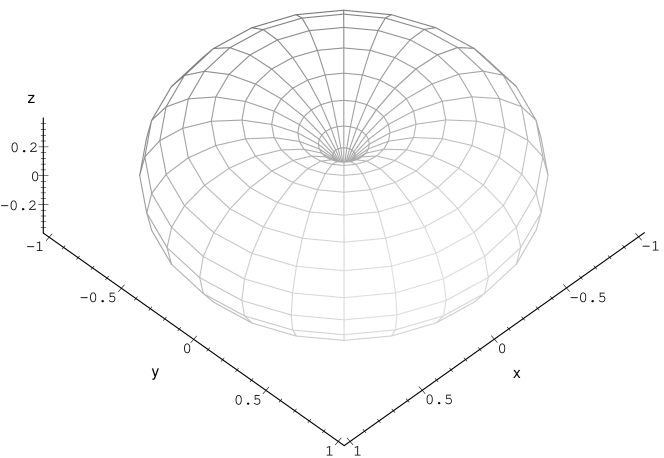
Fig. 1: The polarization-averaged RMS sensitivity of a bar detector to gravitational waves incident from any direction. The detector is at the origin of the figure and has its symmetry axis along the figure’s $z$ axis. The magnitude of the distance from the origin to the surface in a direction $\hat{n}$ is proportional to the relative response of the detector to radiation incident on the detector from that direction.

Next consider a plane gravitational wave propagating in the $\hat{k}$ direction and define the polarizations of the gravitational wave. Introduce a plane orthogonal to $\hat{k}$. In this plane, spanned by the Cartesian coordinates $\hat{x}^{\prime}$ and $\hat{y}^{\prime}$, the TT-gauge metric perturbation can be written

$$h_{ij}dx^{i}dx^{j}=h_{+}\left({dx^{\prime}}^{2}-{dy^{\prime}}^{2}\right)+2h_{\times}dx^{\prime}dy^{\prime}.$$ (45)

The choice of $\hat{x}^{\prime}$ and $\hat{y}^{\prime}$ is arbitrary: different choices correspond to either or both a rotation of one polarization state into another or a reflection that flips the sign of $h_{\times}$. For definiteness, we choose $\hat{x}^{\prime}$ to be orthogonal to $\hat{z}$ and $\hat{y}^{\prime}$ such that ($\hat{x}^{\prime}$, $\hat{y}^{\prime}$, $\hat{k}$) is a right-handed coordinate system. (In the degenerate case, where $\hat{k}$ is parallel to $\hat{z}$, we choose $\hat{x}^{\prime}$ parallel to $\hat{x}$ and $\hat{y}^{\prime}$ parallel to $\hat{y}$.) With these choices, it is straightforward to show that the response of the bar’s longitudinal mode is proportional to $h$, where

$$h = F_{{}+{}}h_{{}+{}}+F_{\times}h_{\times}$$ (46)

$$F_{{}+{}} = \sin^{2}\theta$$ (47)

$$F_{{}\times{}} = \sin^{2}\theta$$ (48)

$$\cos^{2}\theta = \left(\hat{k}\cdot\hat{n}\right)^{2}$$ (49)

Figure 1 shows the polarization-averaged RMS sensitivity of a right cylindrical acoustic detector to plane waves incident from a given direction. To interpret the figure, imagine a detector at the figure’s origin with its symmetry axis coincident with the figure’s $z$ axis. A plane wave, arriving from direction $\hat{n}$, leads to a detector response proportional to the distance in the direction $\hat{n}$ from the figure’s origin to the surface.

3.3.2 Interferometric detectors.

Interferometric gravitational wave detectors respond when incident gravitational waves cause a differential change in the length of the interferometer arms. Focus attention on interferometers whose arms meet in a right angle. To get a sense of the differential sensitivity of such a detector to radiation of different polarizations incident from different directions, define a right-handed interferometer coordinate system whose origin is the intersection of the arms and whose $x$ and $y$ coordinate directions are in the direction of the arms. Let a plane wave, described by the perturbation

$$h_{ij}dx^{i}dx^{j}=h_{{}+{}}\left(dx^{2}-dy^{2}\right)+2h_{\times}dx\,dy,$$ (50)

be incident on the detector from direction $\hat{z}$. There will be no detector output proportional to $h_{\times}$, since that component of the radiation does not lead to a differential change in the arm lengths; on the other hand, the polarization component proportional to $h_{{}+{}}$ does lead to a differential change in the arm lengths and, correspondingly, to detector output.

Similarly, consider radiation incident on the detector along the interferometer’s $x$ arm:

$$h_{ij}dx^{i}dx^{j}=h_{+}\left(dy^{2}-dz^{2}\right)+2h_{\times}dy\,dz.$$ (51)

Again, the $\times$ polarization mode does not lead to a differential change in the interferometer arm lengths (at first order in $h$); so, the detector is not sensitive to radiation with this polarization. On the other hand, radiation in the ${}+{}$ polarization mode, as we have defined it, leads to changes in the length of the $y$ arm while leaving the $x$ arm length unchanged; consequently, there is a differential change in the interferometer arm length and the detector is sensitive to radiation of this polarization incident from this direction.

To determine in general the coefficients $F_{{}+{}}$ and $F_{\times}$ that describe the response of an interferometric detector to incident plane waves, first describe the polarization modes of radiation incident on the detector relative to the detector coordinate system. In the usual ($\theta$, $\phi$) spherical coordinates associated with the interferometer coordinate system, the incident direction of a plane-wave propagating with wave-vector $\vec{k}$ is

$$\cos\theta \equiv -\vec{k}\cdot\vec{z}/|\vec{k}|,$$ (52)

$$\tan\phi \equiv {\vec{k}\cdot\vec{y}\over\vec{k}\cdot\vec{x}}.$$ (53)

In the plane orthogonal to the radiation propagation direction $\hat{k}$, let the $\hat{x}^{\prime}$ direction be parallel to the $xy$-plane and the $\hat{y}^{\prime}$ direction be orthogonal to $\hat{x}^{\prime}$ so that $(\hat{x}^{\prime},\hat{y}^{\prime},-\hat{k})$ forms a right-handed coordinate system. [In the degenerate case — radiation propagating parallel to the $\hat{z}$ direction — we take $\hat{x}^{\prime}$ parallel to $\hat{x}$ and $\hat{y}^{\prime}$ such that $(\hat{x}^{\prime},\hat{y}^{\prime},-\hat{k})$ is right-handed.] In terms of this coordinate system, define the $+$ and $\times$ polarizations of an incident gravitational wave by

$$h_{ij}dx^{i}dx^{j}=h_{+}\left({dx^{\prime}}^{2}-{dy^{\prime}}^{2}\right)+2h_{\times}dx^{\prime}dy^{\prime};$$ (54)

then, the antenna pattern factors $F_{{}+{}}$ and $F_{\times}$ are given by

$$F_{{}+{}} \equiv {1\over 2}\left(1+\cos^{2}\theta\right)\cos 2\phi\cos 2\psi-\cos\theta\sin 2\phi\sin 2\psi,$$ (55)

$$F_{\times} \equiv {1\over 2}\left(1+\cos^{2}\theta\right)\cos 2\phi\sin 2\psi+\cos\theta\sin 2\phi\cos 2\psi.$$ (56)

Figure 2 shows the polarization-averaged RMS sensitivity of a right-angle interferometric detector to plane waves incident from a given direction. The detector is at the origin of the figure, with its arms along the figure’s $\hat{x}$ and $\hat{y}$ axes. The detector’s sensitivity to radiation incident on the detector from direction $\hat{n}$ is proportional to the distance of the surface from the figure’s origin in the direction $\hat{n}$.

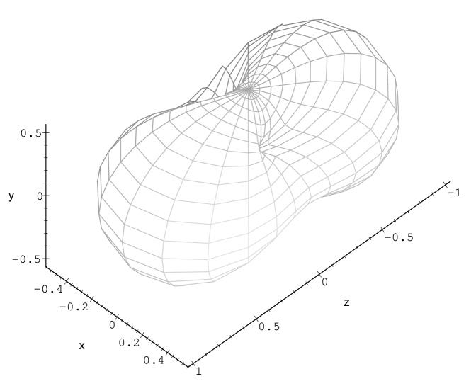
Fig. 2: The polarization-averaged RMS sensitivity of an interferometric gravitational wave detector to radiation incident from any direction. The detector is at the origin of the figure and has its arms aligned with the figure’s $x$ and $y$ axes. The magnitude of the distance from the origin to the surface in a direction $\hat{n}$ is proportional to the relative response of the detector to radiation incident on the detector from that direction, averaged over all polarizations.

3.4 Response Function

The output of a gravitational wave detector is a voltage, $v(t)$, that is linearly related to the incident radiation. Consider a gravitational plane wave, with polarizations $h_{{}+{}}$ and $h_{\times}$, incident on a detector with antenna pattern described by $F_{+}$ and $F_{\times}$. The detector response is given by

$$v(t) = \int_{-\infty}^{t}d\tau\,h(\tau)K(t-\tau),\qquad\mbox{where}$$ (57)

$$h(t) = F_{+}h_{+}(t)+F_{\times}h_{\times}(t)$$ (58)

and $K$ is the kernel of the linear transformation.

It is instructive to express this convolution in the frequency domain:

$$v(t)=\int_{-\infty}^{\infty}df\,\widetilde{h}(f)\widetilde{K}^{*}(f)\exp\left(2\pi ift\right),$$ (59)

where

$$\widetilde{g}(f)\equiv\int_{-\infty}^{\infty}dt\,g(t)\exp(-2\pi ift)$$ (60)

and we have assumed that $K(\tau)$ vanishes for negative $\tau$. From equation 59 we see that the response of the system — the output voltage — depends on the frequency of the incident radiation: depending on the character of the detector, the response may be relatively large for some frequencies and relatively small for others.

As an example, consider two equal masses $M$ connected by a spring (spring constant $\omega_{0}^{2}M$, quality factor $Q$). Denote the equilibrium separation by $L$. A passing gravitational wave of appropriate polarization disturbs the equilibrium separation of the system. The net result is that the passage of a gravitational wave acts as a driving force on the system’s normal mode:

$$\ddot{x}+{\omega_{0}\over Q}\dot{x}+\omega_{0}^{2}x={1\over 2}L\ddot{h},$$ (61)

where $x$ is the difference between the actual and equilibrium separation.

Suppose that we instrument this system with strain gauges to produce an output voltage $v(t)$ proportional to $x(t)$, the deviation from equilibrium separation. How is $v(t)$ (i.e., $x(t)$) related to $h(t)$? In the frequency domain we see that

$$\widetilde{v}(f)\propto{f^{2}\over f_{0}^{2}-f^{2}+iff_{0}/Q}\widetilde{h}(f),$$ (62)

where

$$f_{0}=\omega_{0}/2\pi.$$ (63)

The output voltage for excitations near the resonance can vary dramatically as a function of frequency.

The response function we have just described is equivalent conceptually to that of a modern acoustic detector: the radiation manifests itself as a driving force on the system’s normal modes and the response is a strong function of the frequency in the neighborhood of the resonances.

The response function of an interferometric detector is quite different. For an interferometer, at frequencies much below the round-trip travel time (but greater than the pendulum frequency of the suspended mirrors and beam-splitter) the detector response is independent of frequency; only when the frequency becomes comparable to or larger than the round-trip light travel time in an interferometer arm does the response vary with frequency.[28]

The amplitude of the response determines those frequencies where an incident gravitational wave of unit amplitude gives relatively large amplitude output and where it gives relatively small amplitude output. It is not, however, the case that relativity large amplitude output corresponds to relatively large sensitivity, if by sensitivity we mean greater ability to detect. To address the question of sensitivity, we must turn to yet a different aspect of a detector’s function: its noise.

3.5 Noise

The output channel of a gravitational wave detector is always alive with random fluctuations — noise — even in the absence of a gravitational wave signal. In a perfect world noise would arise exclusively from fundamental physical processes: e.g., fluctuations owing to the finite temperature of the detector, counting statistics of individual photons on a photo-detector, etc. In the less than perfect world in which we live there will be other contributions to the detector noise, beyond these fundamental processes, that arise from the imperfect construction of the detector (e.g., bad electrical contacts), imperfections in the materials used to construct the detectors (e.g., mechanical creep and strain release), and from the detector’s interaction with the (non-gravitational wave) environment (e.g., seismic vibrations, electromagnetic interactions, etc.).

Detection of gravitational waves requires that we be able to distinguish, in the detector output, between signal and noise. This requires that we have characterized the noise (and not only the signal). Since noise is intrinsically random in character, that characterization is in terms of its statistical properties. Some of these statistical properties we can predict, model or anticipate a priori, based on the detector design; nevertheless, it is important to realize that an experimental apparatus is a real thing made in the real world and will never behave ideally. While a large part of the experimental craft involves building instruments that operate as close as possible to their theoretical limits or prior expectations, the final characterization of a detector will always be determined or verified empirically. In this section we describe something of how noise in gravitational wave detectors is characterized.

3.5.1 Correlations

Just as a probability distribution is fully characterized by its moments, so the random output of a gravitational wave detector can be fully characterized by its correlations. The $N$-point correlation function describes the mean value of the product of the detector output sampled at $N$ different times. Mean, in this case, refers to an ensemble average, where the ensemble is an infinite number of identically constructed detectors. Denoting by $n(t)$ the noisy output of a gravitational wave detector in the absence of any signal, the $N$-point correlation function of the noise distribution is given by

$$C_{N}(\tau_{0},\ldots,\tau_{N-1})=\overline{n(\tau_{0})\ldots n(\tau_{N-1})},$$ (64)

where the over-bar signifies an ensemble average, which is also referred to as an average across the process.

As a practical matter ensemble averages are impossible to realize experimentally: one rarely has the opportunity of working with even two similar detectors, let alone an infinite number of identical ones. Thus, while a handy theoretical construct, the general set of correlation functions is not of great practical use in characterizing the behavior of a real detector.

3.5.2 Stationarity

If, however, the behavior of the detector noise does not depend significantly on time — i.e., the noise is stationary — then the utility of the correlation function as a practical tool for characterizing detector noise increases dramatically. When the noise character is, figuratively, the same today as it was yesterday and as it will be tomorrow, then the detector yesterday (or an hour, or a minute, or a second ago) can be regarded as an identical copy of the detector we are looking at now, and both are identical copies of the detector tomorrow. Consequently, in the spirit of the ergodic theorem, we can replace the average across the process — the ensemble average — with an average along the process — a time average. The $N$-point correlation function is then a function of the difference in time between the $N$ samples:

$$C_{N}(\tau_{1},\ldots,\tau_{N-1})=\lim_{T\rightarrow\infty}{1\over T}\int_{t_{0}-T}^{t_{0}}n(t)n(t-\tau_{1})\cdots n(t-\tau_{N-1})\,dt.$$ (65)

Of course, perfect stationarity is an impossible requirement. As a practical matter, what we require is that the noise process be stationary over a suitably long period. Let’s try to make that concept more quantitative. To simplify the discussion, assume (without loss of generality) that the noise process has zero mean. Consider first the two-time correlation function of a stationary process:

$$C_{2}(\tau)=\lim_{T\rightarrow\infty}{1\over T}\int_{t_{0}-T}^{t_{0}}n(t)n(t-\tau)\,dt.$$ (66)

For sufficiently large $\tau$ we expect intuitively that $C_{2}(\tau)$ should vanish: the output now should be effectively uncorrelated with the output in either the distant past or the distant future. This will also be the case for the higher-order moments as well: for sufficiently large $\tau_{k}$ (any $k$), the correlation function $C_{N}$ should vanish. Thus, we don’t need to require perfect stationarity; rather, we require only that the statistical character be approximately stationary, varying significantly only over times long compared to the longest correlation time. In that case, we can approximate the correlations $C_{N}$ by averaging, as in equation 66, over finite periods.

3.5.3 Gaussian Noise

Noise from fundamental processes tends to be either Gaussian (i.e., originating from contact with a heat bath or some dissipative process) or Poissonian (e.g., originating in the counting statistics of identical and independently distributed — i.i.d. — events that occur at a fixed, average rate). For the gravitational wave detectors under construction, the intrinsically Poissonian processes (e.g., photon counting statistics) have rates so high that they can be treated as Gaussian and we do so here and below.

One way to think about the detector noise is as a superposition of a Gaussian and approximately stationary component, a (hopefully lower amplitude) non-Gaussian, but still stationary component, superposed finally with a non-stationary component. General statements cannot be made about the non-Gaussian or non-stationary components: they differ from instrument to instrument and environment to environment and can only be characterized empirically. The characterization of the Gaussian-stationary component, however, is remarkably simple and has a useful physical interpretation, which we review in this and the next subsection. (For more information and detail, see Finn[29].)

Up to now we have considered the output of a detector as an analog process: i.e., one that is continuous in time. In fact, the output we observe will have been sampled discretely at some sampling rate $f_{s}$, chosen to be something more than twice as great as the maximum frequency of interest for the detector output. So, instead of writing the noise at the detector output as $n(t)$ we write

$$n[k]\equiv n(t_{k}),$$ (67)

where

$$t_{k}=t_{0}+k\Delta t$$ (68)

for constant $\Delta t$.

When the noise in the detector is Gaussian and stationary, any single sample $n[j]$ of the detector output is drawn from a normal distribution with a mean and variance that are independent of when the sample was taken. Without loss of generality we can assume that the mean $\overline{{n}}$ vanishes, in which case

$$P(n[j])={\exp\left[-n[j]^{2}/2\sigma^{2}\right]\over\sqrt{2\pi\sigma^{2}}}.$$ (69)

We understand the variance $\sigma^{2}$ of the distribution to be the ensemble average of the square of the detector noise:

$$\sigma^{2}=\overline{n[j]^{2}}.$$ (70)

Equation 69 holds true for each sample $n[j]$; consequently, the joint probability that the length $N_{T}$ sequence of samples $n[j]$, $j$ running from 1 to $N_{T}$, is a sample of detector noise is given by the multivariate Gaussian distribution

$$P(n[1],n[2],\ldots,n[N_{T}])={\exp\left[-{1\over 2}\sum_{j,k=0}^{N_{T}-1}n[j]\left|\left|{\bf C}^{-1}\right|\right|_{jk}n[k]\right]\over\sqrt{\left(2\pi\right)^{N_{T}}\det||{\bf C}||}}$$ (71)

In place of the variance $\sigma^{2}$ that appears in the exponent of equation 69 is the covariance matrix ${\bf C}$. (The matrix ${\bf C}^{-1}$ that appears in equation 71 is, by construction, positive definite; consequently, it is non-singular and invertible.) Similarly, in place of the factor $\sigma^{2}$ that appears in the denominator of equation 69 is the determinant $\det||{\bf C}||$.

The mean over the product $n[j]n[k]$ is the value of the correlation function $C_{2}(t_{j}-t_{k})$; it is also just the value of the $jk$ element of the covariance matrix $\left|\left|C\right|\right|$:

$$C_{2}[j-k]=\overline{n[j]n[k]}=\left|\left|{\bf C}\right|\right|_{jk}.$$ (72)

Since the detector noise is also assumed to be stationary, $\left|\left|{\bf C}\right|\right|_{jk}$ can depend only on the difference $j-k$; correspondingly, ${\bf C}$ is constant on its diagonals: i.e., it is a Toeplitz matrix. Consequently, it is fully characterized by the sequence $c[k]$ of length $2N_{T}-1$ whose elements are the first row and column of ${\bf C}$:

$$c[j-k]=\left|\left|{\bf C}\right|\right|_{jk}=C_{2}(t_{j}-t_{k}).$$ (73)

The sequence $c$ and the process mean (which we have assumed to vanish) fully characterize the random process. The sequence $c$, however, is just the two-time correlation function of the detector output! Thus, the two-time correlation function $C_{2}$ fully characterizes a Gaussian stationary process: all the higher order correlation functions $C_{N}$ either vanish (for odd $N$) or are expressible as sums of products of $C_{2}$. Once we have determined $C_{2}$, then, we have completely determined the character of the Gaussian noise process.

3.5.4 Likelihood function

In the last section we evaluated

$$P(v|0)\equiv\left(\begin{array}[]{l}\mbox{probability of observing}\\ \mbox{output sequence $v$ assuming}\\ \mbox{no signal is present}\end{array}\right)$$ (74)

for Gaussian-stationary detector noise. Since the detector is linear, the probability

$$P(v|h)\equiv\left(\begin{array}[]{l}\mbox{probability of observing}\\ \mbox{output sequence $v$ assuming}\\ \mbox{signal $h$ is present}\end{array}\right)$$ (75)

is just

$$P(v|h)=P(v-v_{h}|0),$$ (76)

where $v_{h}$ is the detector response to the gravitational wave signal $h$. The ratio of these two probabilities,

$$\Lambda(v|h)\equiv{P(v|h)\over P(v|0)},$$ (77)

termed the likelihood function, is the odds that the data $v$ is a combination of signal $v_{h}$ and noise, as opposed to a noise alone. For a given observation $v$ the likelihood can be viewed as a function of hypothesized signal $h$, in which case it has a convenient interpretation in terms of plausibility: in particular, $\Lambda(v|h)$ can be interpreted as the plausibility that the signal $h$ is present given the particular observation $v$. (The likelihood is not, however, a probability.) This meaning of the likelihood is independent of the statistical character of the noise. The difficulty, if the noise is not Gaussian-stationary, is in evaluating $\Lambda$.

3.5.5 The two-time correlation function

The correlation function $C_{2}(\tau)$ describes the statistical relationship between pairs of samples drawn from the random process $n(t)$ at times separated by an interval $\tau$. Given two samples separated in time by $\tau$, a non-zero correlation $C_{2}(\tau)$ corresponds to an increased ability to predict the value of one member of the pair given the other.

The correlation function $C_{2}(\tau)$ is bounded by $\pm{}C_{2}(0)$, suggesting that we define the correlation coefficient

$$R_{2}(\tau)\equiv C_{2}(\tau)/C_{2}(0),$$ (78)

which is bounded by $\pm 1$. If the correlation coefficient is zero for some $\tau$, then samples taken an interval $\tau$ apart are entirely uncorrelated: knowledge of one does not lead to any increased ability to predict the other. A positive correlation coefficient tells us that the two samples are more likely close to each other in magnitude and sign than not, while a negative correlation coefficient tells us that the two samples are likely close to each other in magnitude but of opposite sign. The larger the coefficient magnitude the greater the tendency. When the correlation coefficient is unity then the correlation is perfect: i.e., when it is $+1$ the two samples are always equal, and when it is $-1$ the two samples are always of equal magnitude but opposite sign.

3.5.6 Noise Power Spectral Density

Consider for a moment a simple harmonic oscillator — e.g., a pendulum — coupled weakly to a heat bath. The heat bath excites the oscillator so that its mean energy is $k_{B}T$. Since the coupling to the heat bath is weak, the phase of the oscillator progresses nearly uniformly in time with rate $\omega_{0}$ corresponding to the oscillator’s natural angular frequency. Over long periods, however, the continual, random excitations of the oscillator cause the phase to drift in a random manner from constant rate.

Now suppose that we sample the position coordinate of the oscillator at intervals separated by exactly one period $2\pi/\omega_{0}$. Since the coupling to the heat bath is weak the samples are very nearly identical: in fact, were it not for the contact with the heat bath, they would be exactly identical. Thus, we expect that the correlation coefficient corresponding to an interval equal to an oscillator period should be nearly unity. Continuing to focus on samples taken at intervals equal to exact multiples of the period, we expect that the correlation coefficients should remain large for small multiples, but should decrease as the interval increases since contact with the heat bath will lead, as time increases, to greater drift in the phase.

On the other hand, suppose that we sample the position coordinate of the oscillator at intervals separated by exactly odd integer multiples of a half-period $\pi/\omega_{0}$. Now we expect the correlation coefficient to be nearly equal to $-1$ for small intervals, decreasing in magnitude to $0$ as the interval increases.

Contact with a heat bath can take place in many ways, leading to subtly different correlation functions. Figure 3 shows the correlation function corresponding to two different kinds of heat bath contact: that which leads to velocity damping and that which leads to structural damping[30]. Note how, pictured in this way, there is apparently little difference between these two damping measures.

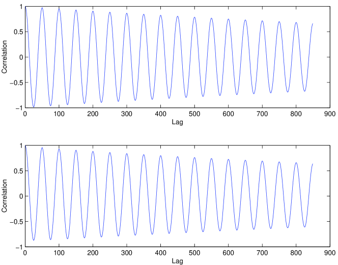
Fig. 3: The correlation functions for a harmonic oscillator in contact with a heat bath. Contact with a heat bath leads to damping; the nature and degree of the contact determine the character of the system’s noise. In this figure we show the correlation function, over several periods, for two different kinds of heat bath contact with the same on-resonance damping. The upper panel corresponds to a viscous damped harmonic oscillator; the lower panel corresponds to a structurally damped oscillator. The difference between the two correlation functions is apparently very subtle.

Since the correlation function is so oscillatory we are immediately led to consider its Fourier transform. In this case, since $C_{2}(\tau)$ is an even function of the lag $\tau$, we consider the cosine transform, which we term the one-sided power spectral density:

$$S_{v}(f)=4\int_{0}^{\infty}d\tau\,C_{2}(\tau)\cos(2\pi f\tau).$$ (79)

(One-sided refers to the fact that, in choosing a cosine transform, we have effectively folded the power in negative frequencies into the power at positive frequencies; so, the $S_{v}(f)$ includes the power at frequencies whose magnitude is $|f|$.) Figure 4 shows the power spectral densities corresponding to the correlation functions of figure 3. The strongly oscillatory nature of these functions shows up as a large peak at the oscillator resonant frequency (normalized to unity). In addition, however, the PSD shows clearly the very different off-resonance character of the noise. Noise from a structurally damped system rises in amplitude as the frequency falls below resonance, unlike the noise contribution from a viscously damped system; similarly, noise from a structurally damped system falls more steeply with frequency above resonance than does the noise from a viscously damped system. To see the same in the correlation function would require close inspection of the trends of the correlation function envelopes over very long lags.

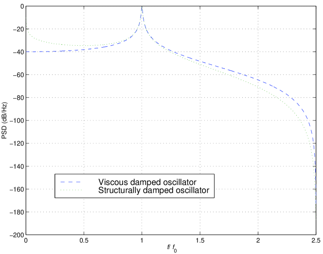
Fig. 4: The power spectral density of the two processes whose correlation functions are shown in figure 3. Note that, while the correlation functions appear very similar as functions of time, strong differences show up in the power spectral densities as functions of frequency.

Thus, even though it is completely equivalent to the correlation function, the power spectral density is often a more useful characterization of the noise character. In the case of Gaussian noise its equivalence to the correlation function guarantees it is also a full characterization of the detector noise. When the noise is not Gaussian, there are analogous spectra associated with the higher order correlations: for example, the bispectrum is the 2-dimensional Fourier transform of $C_{3}(\tau_{1},\tau_{2})$,

$$\mbox{Bi}(f_{1},f_{2})=\int_{-\infty}^{\infty}d\tau_{1}e^{-2\pi if_{1}t_{1}}\int_{-\infty}^{\infty}d\tau_{2}\,e^{-2\pi if_{2}t_{2}}\,C_{3}(\tau_{1},\tau_{2}),$$ (80)

and so on. These higher order spectra and their magnitudes play the same role for the higher-order correlation functions as the power spectral density plays for the auto-correlation function.

3.6 Signal-to-noise ratio

When is a gravitational wave “detectable”? We haven’t yet explored the meaning of “detection” qualitatively, let alone quantitatively; nevertheless, we have an intuitive feeling that a signal ought to be detectable if the detector’s response to the signal is greater than the intrinsic noise amplitude. Let’s develop that idea a bit.

Suppose that we have a detector with noise power spectral density $S_{v}(f)$ and particular output $v(t)$, which consists of a signal $v_{h}(t)$ superposed with detector noise $v_{n}(t)$. The variance of $v(t)$, over an interval $[0,T]$, is

$$\sigma^{2}_{v} = {1\over T}\int_{0}^{T}dt\,v(t)^{2}$$ (81)

$$= {2\over T}\int_{0}^{\infty}df\,\left|\widetilde{v}(f)\right|^{2}.$$ (82)

The noise is a random process; so, then, is $\sigma^{2}_{v}$. Focus on the ensemble average of $\sigma^{2}_{v}$ and look in the frequency domain:

$${d\overline{\sigma^{2}_{v}}\over df} = {2\over T}\overline{\left|\widetilde{v}(f)\right|^{2}}$$ (83)

$$= {2\over T}\left(\overline{\left|\widetilde{v}_{n}(f)\right|^{2}}+\left|\widetilde{v}_{h}(f)\right|^{2}\right)$$ (84)

where the final equality follows when we recognize that the noise is independent of the signal. The contribution to the mean signal variance thus consists of separate contributions from the signal and from the noise.

The ratio

$${\left|\widetilde{v}_{h}(f)\right|^{2}\over\overline{\left|\widetilde{v}_{n}(f)\right|^{2}}}$$ (85)

evidently tells us which — signal or noise — is expected (note ensemble average!) to contribute more to the amplitude of the detector output in a unit bandwidth about frequency $f$. We can compute a similar, dimensionless quantity over the full bandwidth:

$$\int_{-\infty}^{\infty}df\,{\left|\widetilde{v}_{h}(f)\right|\over\overline{\left|\widetilde{v}_{n}(f)\right|}/T}=4\int_{0}^{\infty}df\,{\left|\widetilde{v}_{h}(f)\right|\over S_{v}(f)}$$ (86)

tells us which of the signal $v_{h}$ or the noise $v_{n}$ is expected to contribute more to the variance of the output $v$.

Given a particular sample of detector output $v$ we don’t know, a priori, what part is $v_{n}$ and what part (if any) is $v_{h}$. Consider a quantity that we can calculate directly from the detector output $v$:

$$\rho^{2}\equiv 4\int_{0}^{\infty}df\,{\left|\widetilde{v}(f)\right|^{2}\over S_{v}(f)}.$$ (87)

The integrand is evidently the ratio of the actual contribution to the signal variance in a unit band about frequency $f$ to the contribution that would be expected, in the same band, from noise alone. Not surprisingly, the ensemble mean $\overline{\rho^{2}}$ is

$$\overline{\rho^{2}}=1+4\int_{0}^{\infty}df\,{\left|\widetilde{v}_{h}(f)\right|\over S_{v}(f)}$$ (88)

We refer to $\rho^{2}$ as the signal-to-noise ratio, or SNR.

Our construction of $\rho^{2}$ has been physically motivated. It turns out, however, that exactly this same quantity arises from a consideration of the probability $P(v|0)$, which we explored in §3.5.3. In that section we found, for Gaussian-stationary noise,

$$P(v|0)={\exp\left[-{1\over 2}\sum_{j,k=0}^{N-1}v[j]\left|\left|{\bf C}^{-1}\right|\right|_{jk}v[k]\right]\over\sqrt{2\pi\det\left|\left|{\bf C}\right|\right|}}$$ (89)

With just a little algebra, however, the argument of the exponential can be rewritten as[31]

$$\sum_{j,k=0}^{N-1}v[j]\left|\left|{\bf C}^{-1}\right|\right|_{jk}v_{h}[k] = \Re\left[{1\over 2N-1}\sum_{j=-(N-1)}^{N-1}{\left|\widetilde{V}[j]\right|^{2}\over\widetilde{c}[j]}\right]$$ (90)

where the periodic sequence $\widetilde{g}[j]$ is related to the discrete Fourier transform of the sequence $g[k]$:

$$\hat{g}[j]=\sum_{k=-(N-1)}^{N-1}e^{-2\pi ikj/(2N-1)}{g}[k]$$ (91)

and $V[k]$ is just $v[k]$ zero-padded for negative $k$:

$$V[k]=\left\{\begin{array}[]{ll}v[k]&\mbox{for $k\geq 0$}\\ 0&\mbox{for $k<0$}.\end{array}\right.$$ (92)

These summations can be regarded as approximations to integrals, in which case

$$\Re\left[{1\over 2N-1}\sum_{j=-(N-1)}^{N-1}{\left|\widetilde{V}[j]\right|^{2}\over\widetilde{c}[j]}\right]\propto\int_{0}^{\infty}df\,{\left|\widetilde{V}\right|^{2}\over S_{h}(f)}.$$ (93)

Hence, the SNR associated with the observed detector output $v$ is closely related to the probability that $v$ is a sample of just detector noise, with no gravitational-wave signal present. The larger $\rho^{2}$, the smaller this probability. Should we observe detector output with large $\rho^{2}$, then, we are not too far wrong to be suspicious that we have seen evidence for gravitational waves.

To make this last judgment — which involves making quantitative the notion of “large” $\rho^{2}$ — we need to know the probability distributions of the SNR in both the presence and absence of a signal: after all, since noise is a random process there is some non-zero probability that, in any given observation, $\rho^{2}$ will take on any particular value, large or small. We return to consider this point in §4

3.6.1 Matched Filtering

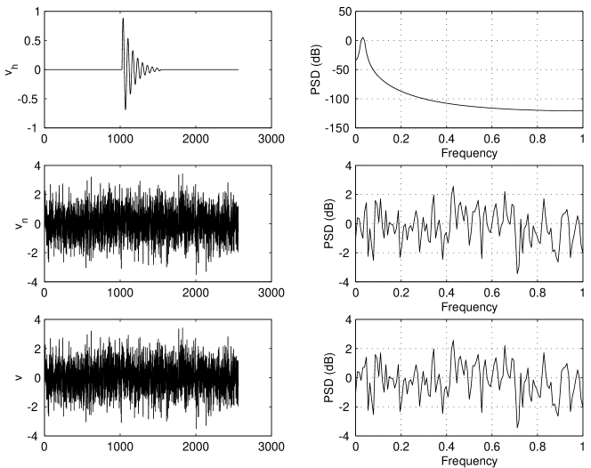
Fig. 5: An imagined gravitational wave signal (upper-left panel), detector noise (middle-left panel) and total detector output (signal$+$noise, lower-left panel). Note how the signal is not evident to the eye in the detector output. The right-hand panels show the power spectra of the corresponding left-hand panels; again, the signal power is not evident relative to the noise power.

Calculating $\rho^{2}$ defined by equation 87 does not require or make use of any information about the gravitational radiation source. Suppose that we know, a priori, the radiation waveform has the shape $V_{h}(t)$, and that the question is whether the corresponding signal $\alpha V_{h}(t-t_{0})$, for some unknown constants $\alpha$ and $t_{0}$, is present in the detector observed output $v(t)$. Can we make use of this information — the signal shape $V_{h}(t)$ — to boost our ability to observe the signal?

The answer is yes. To illustrate, figure 5 shows an imagined $v_{h}$, $v_{n}$ and $v$ equal to $v_{h}+v_{n}$ in the left-hand panels, and the corresponding power spectra in the right-hand panels. For this illustration we have assumed that the noise is white across the detector bandwidth. The signal is not apparent to the eye in either $v$ or its power spectrum $P_{v}(f)$. Figure 6 shows, in the top panel, the filter output when just $v_{h}$ is passed through the filter $K$ with impulse-response $V_{h}$ set equal to $v_{h}$:

$$v^{\prime}(t) = \int_{-\infty}^{t}d\tau\,v(\tau)K(t-\tau)$$ (94)

$$= v^{\prime}_{n}(t)+v^{\prime}_{h}(t)$$ (95)

where

$$K(\tau) = v_{h}(t)$$ (96)

$$v^{\prime}_{n}(t) = \int_{-\infty}^{t}d\tau\,v_{n}(\tau)V_{h}(t+\tau)$$ (97)

$$v^{\prime}_{h}(t) = \int_{-\infty}^{t}d\tau\,v_{h}(\tau)v^{\prime}_{h}(t+\tau).$$ (98)

Without loss of generality we assume $v_{h}$ is non-zero only for positive $t$. The filtered detector output $v^{\prime}(t)$ consists of a signal contribution $v^{\prime}_{h}(t)$ and a noise contribution $v^{\prime}_{n}(t)$. These are shown in the top and middle panels of figure 6, respectively. The bottom panel of figure 6 shows the filter output $v^{\prime}$ (equal to $v^{\prime}_{h}+v^{\prime}_{n}$). The presence of the “signal” $v^{\prime}_{h}$ is now much more evident.

The filter we have chosen has reduced the total power in the noise relative to that in the signal. How it does this is apparent by considering the power spectra in figures 5 and 6. In figure 5, the power in $v_{h}$ is seen to be confined to a very narrow bandwidth about the frequency of the damped sinusoid. At its peak the signal power is about 5 dB greater than noise power. Nevertheless, the total noise power, integrated over the full bandwidth, is much greater than the signal power and, consequently, the signal is overwhelmed by the noise (cf. the bottom panel of figure 5).

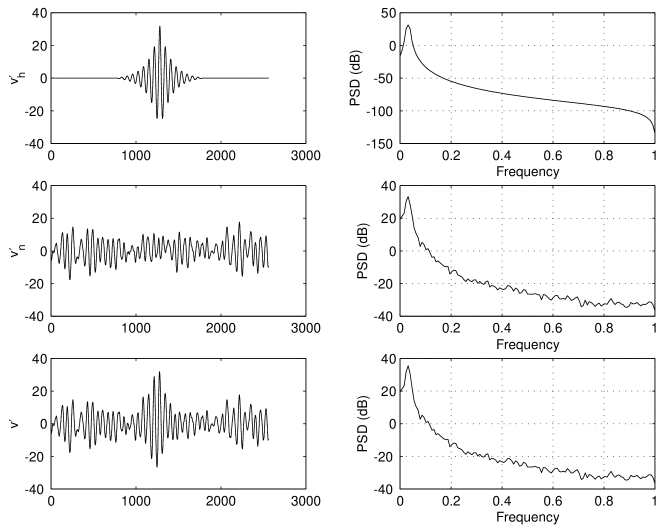
Fig. 6: The output of the filter described in equation 95 when just the signal $v_{h}$ is filtered (upper panel) and when the detector output, consisting of signal and noise, is filtered (lower panel). In contrast to the lower-right panel of figure 5, the “signal” (i.e., the upper panel) is quite evident even in the presence of noise.

Now consider $v^{\prime}$. The filter applied to the signal has the impulse response of the signal, or the squared magnitude frequency response given by the power spectrum in the top panel of figure 5. This is matched to the signal, in the sense that the power passed is in the band where the signal power is large and the power stopped is in the band where the signal power is small. Thus, what survives in $v^{\prime}$ is the signal power, together with only that noise power in the narrow band where the signal power is large. The signal to noise of the filtered detector output $v^{\prime}$ is correspondingly much higher in the presence of the signal than is the signal to noise ratio of $v$.

This example is illustrative. In fact, we can ask, for an arbitrary signal $v_{h}$ embedded in noise with power spectrum $S_{v}(f)$, for the linear filter that maximizes the ratio of the mean-square signal contribution to the mean-square noise contribution. That filter is referred to as the Wiener matched filter; in the frequency domain and for weak signals it is (up to an overall constant)

$$\widetilde{K}(f)={\widetilde{v}_{h}^{*}(f)\over S_{h}(f)}.$$ (99)

More generally, additional information is always useful for increasing the our ability to detect a signal. This is true even that information is not as complete as knowing the waveform. For example, consider the case where we know the signal spectrum, but not its waveform. In the frequency domain, we thus know the signal amplitude at each frequency, but not the corresponding phase. In the case where the waveform is known, we constructed the filter making full knowledge of both amplitude and phase information. We can also construct a filter that passes power in a given bandwidth, without regard to its phase. This filter will emphasize power in the bands where the ratio of signal power to noise power is relatively large over bands where the ratio is small; consequently, it will increase our ability to detect a signal whose spectrum is known in the same way that a matched filter increases our ability to detect a signal whose waveform is known.

3.7 The effective noise power spectral density

How does one compare different detectors, with different response functions and different noise power spectral densities?

One possibility is the “performance benchmark”: choose a prototypical source, evaluate the signal-to-noise that the source would give in the different detectors, and determine finally which detector is most likely to observe the source at a given level of confidence [32].

This kind of judgment depends critically on the source: using different sources as your benchmark can lead to different conclusions. For example, sources whose power is concentrated at different frequencies focus attention on the detector noise at those frequencies. Thus, while benchmarking detectors against particular sources can be a powerful tool for comparing their relative performance, it is also a tool with a very narrow focus. We need some other way to compare the capability of detectors with a less specific emphasis on source.

An important tool for making this more general comparison is the effective power spectral density $S_{h}(f)$,

$$S_{h}(f)\equiv{S_{v}(f)\over|R(f)|^{2}},$$ (100)

where $R(f)$ is the detector response function and $S_{v}(f)$ is the detector noise power spectral density. The quantity $S_{h}(f)$ describes an effective detector noise: it is the power spectral density of a stochastic gravitational wave signal that would have to be applied to a noise-free detector in order that the corresponding response have power spectral density $S_{v}(f)$. Over frequency bands where $S_{h}(f)$ is small, the detector is relatively sensitive; over frequency bands where it is large, the detector is relatively insensitive.

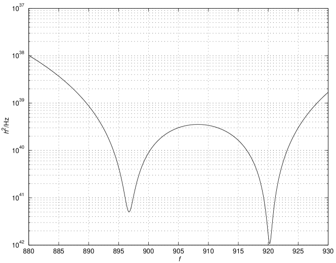
Fig. 7: The power spectral density of an effective stochastic gravitational wave signal that would mimic the noise in the output of a modern bar detector. Plotted is $\sqrt{S_{h}(f)}$ vs. frequency $f$.

The effective power spectral density $S_{h}(f)$ has both a source and detector independent meaning, making it a particularly useful quantity for comparing gravitational wave detectors or for comparing a detector to a source. With it, one can rank detectors according to their overall noise in a given bandwidth, e.g.,

$$\overline{h^{2}}_{n}(f_{1},f_{2})=\int_{f_{1}}^{f_{2}}df\,S_{h}(f),$$ (101)

or define an effective band $(f_{0}-\Delta f/2,f_{0}+\Delta f/2)$ over which the detector has greatest sensitivity, e.g.,

$$f_{0} \equiv {\int_{0}^{\infty}df\,f/S_{h}(f)\over\int_{0}^{\infty}df/S_{h}(f)}$$ (102)

$$\left(\Delta f\right)^{2} \equiv {\int_{0}^{\infty}df\,(f-f_{0})^{2}/S_{h}(f)\over\int_{0}^{\infty}df/S_{h}(f)}.$$ (103)

Finally, since the noise is referred directly to the amplitude of incident gravitational radiation, one can calculate the expected SNR of a given signal in the detector without reference to the detector’s response function:

$$\overline{\rho^{2}} = 1+4\int_{0}^{\infty}df\,{\left|R(f)\widetilde{h}(f)\right|^{2}\over S_{v}(f)}$$ (104)

$$= 1+4\int_{0}^{\infty}df\,{\left|\widetilde{h}(f)\right|^{2}\over S_{h}(f)}.$$

Figure 7 shows the modeled $S_{h}(f)$ for a modern bar detector, while figure 8 shows $S_{h}(f)$ for a model of the first-generation LIGO instrumentation. Note how the bar detector noise is particularly small in two narrow bands about the resonant frequencies of the two mode system consisting of the bar and its transducer, while the interferometer achieves its peak sensitivity over a much broader bandwidth.

3.7.1 An aside: noise in bar detectors

It is a common misconception that bar detectors are intrinsically narrow-band detectors. While the amplitude of a resonant detector’s response is greatest for signal power in the neighborhood of the resonance, the thermal excitation of the bar is also concentrated in this band as well. The net result is that the contribution of the bar’s thermal noise to the power spectral density expressed in units of $h^{2}/\mbox{Hz}$ is effectively independent of frequency.

To understand how resonant detectors become narrow band instruments, consider how the signal appears in the electronics that follow the transducer. The resonant character of the detector leads to large amplitude motion for signal power near the resonant frequency and small amplitude motion for signal power far from the resonance. Correspondingly, the amplified signal is large near to, and small far from, the resonance. The amplifier contributes its own noise, however, which is approximately white at the amplifier output. Thus, compared to the signal presented for amplification, the amplifier noise is relatively large far from resonance and relatively small near to resonance.

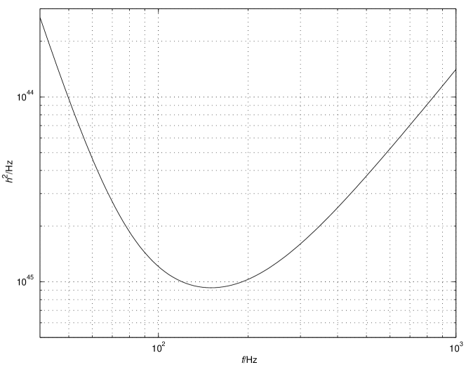
Fig. 8: The power spectral density of an effective stochastic gravitational wave signal that would mimic the noise in the output of first generation LIGO instrumentation. Plotted is $\sqrt{S_{h}(f)}$ vs. frequency $f$.

In present-day resonant cryogenic detectors the bandwidth is limited by amplifier noise, referred back to $h$ through the response function.

Since it is the amplifier noise, when referred back to $h$ through the response function of the resonant bar, that limits the instrument bandwidth, why make the bar resonant at all? The purpose of making the detector resonant is to provide mechanical amplification for the signal, so that, at least in a narrow bandwidth, it is much stronger then the limiting noise source: amplifier noise. Signal power at or near resonance leads to a large excitation of the bar, which translates into a large input to the amplifier; thus, the resonance of the bar amplifies the incident gravitational wave signal relative to all the noise sources that follow, including the limiting amplifier noise.

3.8 Conclusion

Gravitational wave detectors are characterized by their antenna patterns, which describe their differential sensitivity to radiation incident from different directions and with different polarizations, their response functions, which describe the differential amplitude of their response to signals of different frequency, and the character of their noise.

The distinction between the response function and the antenna pattern is sometimes an artificial one: the response function can (and for interferometric detectors, does) depend on the incident direction of the radiation.

Much of the experimental craft is devoted to making the detector noise approximately stationary and Gaussian (or in making the signal so large that the character of the noise is not significant for measurements of interesting precision). Stationary noise can be characterized by evaluating the correlations among samples taken at different relative times. For Gaussian noise, all the correlations are known once the pairwise correlation function is measured.

While the correlation functions are good conceptual tools for understanding the character of stationary detector noise, a more useful tool, fully equivalent, is the noise spectrum: the Fourier transform of the correlation function on its time arguments. The noise power spectral density, in particular, is a particularly important and useful tool for characterizing the disposition of detector noise power.

4 Characterizing detection

What does “detection” mean? Let’s try to frame an answer by posing a specific question — e.g., “with what confidence can we conclude that, in the last hour, gravitational waves from a new core collapse supernova in the Virgo cluster of galaxies passed through our gravitational wave detector?” — and exploring its meaning.

It turns out that, straightforward as it seems, there are two different ways of interpreting this question; correspondingly, there are two different meanings that “detection” can take. How we mean the question — or the kind of answer that we want to take away — determines the kind of analysis that we need to undertake with data collected at a gravitational wave detector.

4.1 Learning From Observation

“With what confidence can we conclude that, in the last hour, gravitational waves from a new core collapse supernova in the Virgo cluster of galaxies passed through our gravitational wave detector?”

As with most questions of detection, even before examining our observations we have some expectation of the answer. In this case, we know the rate of supernovae and this leads us to expect, on average, one such core collapse every 4 months; consequently, we believe the probability is approximately $3.4\times 10^{-4}$ that in any given hour — including the last — gravitational waves from a new Virgo cluster supernova were incident on our detector.

Probability, as we have used it here, means degree of belief. In this instance, our degree of belief coincided with the expected frequency of supernova events. This need not always be the case: we can assess degree of belief even when we can’t assess relative frequency. For example, suppose that I have a coin that is known to be heavily biased toward either heads or tails. What is your degree of belief that, when I next flip the coin, it will land heads-up? Without telling you the direction or amount of the bias, you can’t evaluate the expected relative frequency of heads or tails. You can, however, quantify your degree of belief: having no more reason to believe that the bias is toward heads than towards tails, you have no more reason to believe that the coin will, when next flipped, land heads-up than that it will land heads-down. Your degree of belief in either alternative, then, is $1/2$.

One does not have to search either long or hard to find examples from, e.g., astrophysics, where probability as “degree of belief” exists and probability as “expected frequency” does not. For example, what is the probability that there exists a cosmological stochastic gravitational wave signal with a given amplitude and spectrum? In this case, “expected frequency” has no meaning: there is only one Universe, and it either does or does not have a stochastic gravitational wave background of given spectrum and amplitude.

After we examine the output of our gravitational-wave detector, our degree of belief in the supernova proposition may change: we may, on the basis of the observations, become more or less certain that radiation from a supernova passed through our detector. How do observations change our degree of belief in the different alternatives?

To explore how our degree of belief evolves with the examination of observations we need to introduce some notation:

$$H_{0} = \left(\begin{array}[]{l}\mbox{proposition that gravitational waves from a}\\ \mbox{new supernova in the Virgo cluster {\em did not}}\\ \mbox{pass through our detector in the last hour}\end{array}\right),$$ (108)

$${\cal I} = \left(\begin{array}[]{l}\mbox{our prior knowledge of astrophysics, including}\\ \mbox{our best assessment of the supernova rate}\end{array}\right),$$ (111)

$$g = \left(\begin{array}[]{l}\mbox{observations from our gravitational wave detector}\end{array}\right),$$ (113)

$$P(A|B) = \left(\begin{array}[]{l}\mbox{degree of belief in $A$ assuming that $B$ is true}\end{array}\right),$$ (115)

$$\neg{}A = \left(\mbox{logical negation of proposition $A$}\right).$$ (116)

In this notation, $P(H_{0}|{\cal I})$ is the degree of belief we ascribe to the proposition that no gravitational waves from a core collapse supernova in the Virgo cluster passed through our detector in the last hour, given only our prior understanding of astrophysics; similarly, $P(H_{0}|g,{\cal I})$ is the degree of belief we ascribe to the same proposition, give both the observation $g$ and our prior understanding of astrophysics.

To understand how $P(H_{0}|{\cal I})$ and $P(H_{0}|g,{\cal I})$ are related to each other we need to recall two properties of probability. The first is unitarity: probability summed over all alternatives is equal to one. In our example, the two alternatives are that a supernova occurred or it did not:

$$P(H_{0}|g,{\cal I})+P(\neg{}H_{0}|g,{\cal I})=1.$$ (117)

The second property we need to recall is Bayes Law, which describes how conditional probabilities “factor”:

$$P(A|B,C)P(B|C)=P(A,B|C)=P(B|A,C)P(A|C).$$ (118)

Combining unitarity and Bayes Law it is straightforward to show that

$$P(\neg{}H_{0}|g,{\cal I})={\Lambda(g)\over\Lambda(g)+P(H_{0}|{\cal I})/P(\neg{}H_{0}|{\cal I})}$$ (119)

where

$$\Lambda(g) = {P(g|\neg{}H_{0},{\cal I})/P(g|{H}_{0},{\cal I})}$$ (120)

$$P(g|H_{0},{\cal I}) = \left(\begin{array}[]{l}\mbox{probability that $g$ is a sample of}\\ \mbox{detector output when $H_{0}$ is true}\end{array}\right)$$ (123)

$$P(g|\neg{}H_{0},{\cal I}) = \left(\begin{array}[]{l}\mbox{probability that $g$ is a sample of}\\ \mbox{detector output when $H_{0}$ is false}\end{array}\right)$$ (126)

The two probabilities $P(g|H_{0},{\cal I})$ and $P(g|\neg{}H_{0},{\cal I})$ depend on the statistical properties of the detector noise and the detector response to the gravitational wave signal. In some cases they can be calculated analytically; in other circumstances it may be necessary to evaluate them using, e.g., Monte Carlo numerical methods. Regardless of how one approaches data analysis the detector must be sufficiently well characterized that these or equivalent quantities are calculable.

Equation 119 describes how our degree of belief in the proposition $\neg{}H_{0}$ evolves as we review the observations. If $\Lambda$ is large compared to the ratio $P({H}_{0}|{\cal I})$ to $P(\neg{}H_{0}|{\cal I})$ then our confidence in $\neg{}H_{0}$ increases; alternatively, if it is small, then our confidence in $\neg{}H_{0}$ decreases. If $\Lambda$ is equal to unity — i.e., the observation $g$ is equally likely given $H_{0}$ or $\neg{}H_{0}$ — then the posterior probability $P(H_{0}|g,{\cal I})$ is equal to the prior probability $P(H_{0}|{\cal I})$ and our degree of belief in $H_{0}$ is unchanged: we learn nothing from the observation.

We can now answer the question that began this section. We understand confidence to mean degree of belief in the proposition that radiation originating from a new supernova in the Virgo cluster was incident on a particular detector during a particular hour. In response we make a quantitative assessment of our degree of belief in that proposition — the probability that the proposition is true.

4.2 Guessing Natures State

Begin again: “With what confidence can we conclude that, in the last hour, gravitational waves from a new core collapse supernova in the Virgo cluster of galaxies passed through our gravitational wave detector?”

As before, we have the hypothesis $H_{0}$ and its logical negation, $\neg{}H_{0}$. The gravitational waves from a new Virgo cluster supernova either passed through our detector, or they did not. Our goal is to determine, as best we can, which of these two alternatives correctly describes what happened.

We decide which alternative is correct by consulting our observation $g$. Operationally, we adopt a rule or a procedure that, when applied to $g$, leads us to accept or reject $H_{0}$. The question that began this section asks us for our degree of confidence in the most reliable rule or procedure.

There are many procedures that we can choose from. Some are just plain silly: for example, always rejecting $H_{0}$ is a procedure. Similarly, accepting $H_{0}$ if a flipped coin lands heads is a procedure. Some procedures are more sensible: we can calculate a characteristic amplitude from the observation (e.g., a signal-to-noise ratio) and reject $H_{0}$ if the amplitude exceeds a threshold. Nature doesn’t always speak clearly; additionally, some crucial information is often hidden from us. Consequently, no procedure will, in the end, be perfect and every rule will, on unpredictable occasions, lead us to erroneous conclusions. Still, some procedures are clearly better than others: the question is, how do we distinguish between them quantitatively?

Better procedures are those that are less prone to error. Consequently, we focus on the frequency with which different procedures err. For our simple problem, where we want to decide only if we have or have not observed the radiation from a supernova (reject or accept $H_{0}$), there are two kinds of errors a decision procedure can make:

1. If no radiation is present ($H_{0}$ true), the rule may incorrectly lead us to conclude that radiation is present: a false alarm, or type I, error.

2. If radiation is present ($H_{0}$ false), the rule may incorrectly lead us to conclude that radiation is absent: a false dismissal, or type II, error.

The false alarm frequency is generally denoted $\alpha$ while the false dismissal frequency is denoted $\beta$.

If we have an ensemble of identical detectors, each observing simultaneously the same system for which $H_{0}$ (or $\neg{}H_{0}$) is true, and we apply our rule to each observation, then the fraction of observations in the ensemble that lead us to reject (accept) $H_{0}$ is just the false alarm (dismissal) frequency. False alarm and false dismissal frequencies can be interpreted as probabilities: in particular, the probability of our rule giving an incorrect result.

Even in the simple case at hand (a single hypothesis that we must accept or reject), there are at least two distinct kinds of errors that an inference procedure can make. Our measure of a rule’s reliability thus involves at least two dimensions, and may involve more. How, then, do we order rules to settle upon a best, or optimal, rule?

To rank rules we must reduce the several error measures that describe a procedure’s performance to a single figure of merit. How we choose to do this depends on the nature of our problem. In our case, rules that distinguish between $H_{0}$ and $\neg{}H_{0}$ are characterized by their false alarm and false dismissal frequencies; consequently, our criteria for ranking rules should depend on our relative intolerance to false alarms and false dismissals. For example, if we are testing for the presence of antibodies in an effort to diagnose and treat a serious illness, we might be very concerned to keep the false dismissal rate low, and not nearly as worried about a high false alarm rate: after all, a false dismissal might result in death, while a false alarm only in an unnecessary treatment with less serious repercussions. Judges or juries in criminal trials faces different concerns: false dismissals let criminals go free, while false alarms send the innocent to prison — neither alternative being very palatable. Finally, in the case of gravitational wave detection, we may (at least initially) be very concerned to avoid false alarms, even at the risk of falsely dismissing many real signals.

Thus, in order to provide a relative ranking of different inference procedures for detection or parameter estimation we must construct an ad hoc figure of merit that reflects our sensitivity to an incorrect decision. We term the best rule, under that ad hoc criteria, the “optimal” rule. “Optimality”, however, is a relative concept: if the criteria change, the “optimal” rule changes also. In the three examples given above, the criteria might be

• medical diagnosis: fix a maximum acceptable false dismissal rate and choose the rule that, among all rules whose false dismissal rate is so constrained, has the minimum false alarm rate;

• criminal justice: choose a rule whose weighted total error $\alpha\cos\phi+\beta\sin\phi$ is minimized ($\phi$ being a matter of personal choice for an individual judge or juror);

• gravitational wave detection: fix a maximum acceptable false alarm rate and choose the rule that, among all rules whose false alarm rate is so constrained, has the minimum false dismissal rate.

False alarm and dismissal rates describe our confidence in the long-run behavior of the associated decision rule. To understand the implications of this measure of confidence, suppose that we have not one, but $N$ independent and identical detectors all observing during the same hour. We use the same test, with false alarm rate $\alpha$ and false dismissal rate $\beta$, on the observations made at each detector, and find that, of these $N$ observations, $m$ lead us (through our inference rule) to reject $H_{0}$ and $N-m$ lead us to accept $H_{0}$. For a concrete example, suppose $\alpha$ is 1%, $N$ is ten and $m$ is three.

The probability of obtaining this outcome when the signal is absent ($H_{0}$ is true) is the probability of obtaining $m$ false alarms in $N$ trials, or

$$P(m|H_{0},N)={N!\over(N-m)!m!}\alpha^{m}(1-\alpha)^{N-m}.$$ (127)

In our example, $P(m|H_{0},N)$ evaluates to $1.1\times 10^{-4}$. It is thus very unlikely that we would have made this observation if the signal were absent. Does this mean we should conclude the signal is present with, say, $99.99$% confidence?

No! $P(m|H_{0},N)$ describes the probability of observing $m$ false alarms out of $N$ observations. When the signal is present, however (i.e., when $H_{0}$ is false), there are no false alarms and both $\alpha$ and $P(m|H_{0},N)$ are irrelevant. There are, however, $N-m$ false dismissals; thus, the relevant quantity is $P(m|\neg{}H_{0},N)$, the probability of observing $N-m$ false dismissals:

$$P(m|\neg{}H_{0},N)={N!\over(N-m)!m!}(1-\beta)^{m}\beta^{N-m}.$$ (128)

If, in our example, the false dismissal rate $\beta$ is 10%, then the probability of observing seven false dismissals out of ten trials is is $8.7\times 10^{-5}$.

The particular outcome of our example — three positive results out of ten trials — is, in the grand scheme of things, very unlikely; nevertheless, what is important to us is that it is more unlikely to have occurred when the signal is present then when it is absent. Despite the apparently overwhelming improbability of three false alarms in ten trials, it is nevertheless, slightly more likely than the alternative of seven false dismissals in ten trials.

We can now answer the question that began this section. We understand that question to ask for the error rate of the best general procedure for deciding between the alternative hypotheses. There is an implicit assumption regarding the decision criteria, which tells us what “best” means in this context. In the context of these criteria, we calculate the error rates for different inference rules, choose rank the different rules, and find the best rule and its corresponding error rates.

Contrast this with our understanding of the identically worded question as we understood it in the previous subsection. There, we understood confidence to mean the degree of belief that we should ascribe to alternative hypotheses; here, we understand confidence to refer to the overall reliability of our inference procedure. There we responded with a quantitative assessment of our degree of belief in the alternative hypotheses, given a particular observation made in a particular detector over a particular period of time; here we responded with an assessment of the relative frequency with which our rule errs given each alternative hypothesis. There we did not make a choice between alternative hypotheses; rather, we rated them as more or less likely to be true in the face of a particular observation. Here, on the other hand, we do make choices and our concern is with the error rate of our procedure for choosing, averaged over many different observations and many different decisions.

Analyses like the ones in this section, where probability is interpreted as the limiting frequency of repeatable events and the focus is on false alarm and false dismissal frequencies, are termed Frequentist analyses. They have particular utility when it is possible to make repeated observations on identical systems: e.g., particle collisions in an accelerator, where each interaction of particle bunches is a separate “experiment.” Analyses like those in the previous section, where probability is interpreted as degree-of-belief and the focus is on the probability of different hypotheses conditioned on the observed data, are termed Bayesian analyses. Bayesian analyses are particularly appropriate when the observations or experiments are non-repeatable: e.g., when the sources are, like supernovae, non-identical and destroy themselves in the process of creating the signal. In this case we are interested in the properties of the individual systems and would prefer a measure of the relative degree of belief that we should ascribe to, for example, the proposition that the signal originated from a particular point in the sky.

That Bayesian and Frequentist analyses are different does not imply that one is right and the other wrong. Bayesian and Frequentist analyses do not address the same questions; so, they are not required to reach “identical” conclusions. On the other hand, it may well be that one analysis is more appropriate or responsive to our concerns than the other. We can only make the choice of appropriate analysis tools when we understand the distinction between them.

5 Gravitational Radiation Sources

In this section we review briefly some of the different kinds of sources that are, at this writing, thought to be “important” for the generation of large interferometric detectors now under construction. “Important” is a term that requires definition in this context. Clearly, sources that we don’t expect to detect, or to be able to detect, are unimportant. Detectable sources must radiate significant energy in the bandwidth where these detectors are most sensitive (ranging from the tens to hundreds of Hz) over a reasonable observation period. For periodic sources, this is the integrated power over a period of several months to perhaps as much as one to two years; for burst sources, this means that the expected rate of detectable bursts must be at least several per year.

The assessment of source strength and number or rate is difficult to make for most sources. Very often the radiation strength depends on physics and astrophysics that we don’t know or understand in the requisite detail. For all proposed sources the rate, number or even existence of sources whose signal strengths are large enough to be detectable is difficult to ascertain. This is not surprising: what we know of the heavens we know principally through electromagnetic observations; however, it is in the nature of gravitational wave sources that they leave little electromagnetic evidence of their existence.

Finally, since we are, with these instruments, looking at the universe in a fundamentally new way, we must keep an open mind to the possibility of sources unimagined: in this I side with John Haldane, who said (in a different context) “My own suspicion is that the universe is not only stranger than we suppose, but stranger than we can suppose.”

One final note: until now, we have been careful to keep all factors $G$ and $c$ in our expressions for gravitational effects. Here and henceforth, we will write all expressions in units where $G$ and $c$ are unity: e.g., units of length, with conversion factors from grams and ergs to centimeters as given in equations 6 and 7. These conversion factors can be invoked to find expressions in terms of quantities expressed in more conventional units.

5.1 Burst sources

5.1.1 Compact binary inspiral

The source most-talked-about for the interferometric detectors now under construction are binary systems consisting of two compact, stellar mass objects — either neutron stars or stellar mass black holes. Like a rotating dumbbell, a binary star system has a large, accelerating quadrupole moment, which makes it (for its mass) a strong gravitational radiation source. The radiation carries away orbital binding energy and orbital angular momentum, which leads to a faster and more compact orbit. Kepler’s Third Law relates the orbital frequency $f_{\mbox{\small orb}}$, semi-major axis $a$ and total system mass $M$ by

$$f_{\mbox{\small orb}}^{2}={M\over 4\pi^{2}a^{3}}.$$ (129)

Consequently, the radiated power is, in order of magnitude,

$$L\propto\left[Ma^{2}f_{\mbox{\small orb}}^{3}\right]^{2}.$$ (130)

Note that radiated power increases as the orbit decays:

$$L\propto\left(M\over a\right)^{5}.$$ (131)

For binaries that can become sufficiently compact the power radiated gravitationally will, in the end, become large enough to dominate the system’s evolution. Since the radiated power increases as the orbit decays, the system will then decay at an ever increasing rate, with ever increasing radiation amplitude, frequency and power, until the components coalesce. It is the radiation from this inspiral, for binary systems of neutron stars or black holes, that is seen as an important source for the LIGO and VIRGO detectors.

Why compact components, like neutron stars or black holes, and why stellar mass, and not more or less massive? Recall that the proposed interferometric detectors have their greatest sensitivity at approximately 150 Hz. The quadrupole radiation from a binary system is at twice the system’s orbital frequency; correspondingly, if the radiation is to be in the bandwidth of these detectors, the binary systems themselves must exist with orbital frequencies of at least 75 Hz. Kepler’s Third Law places a lower bound for us on the matter density of the components, which must be much greater than the total system mass divided by the cube of the orbital radius:

$$\rho_{1,2} \gg {M\over a^{3}}$$ (132)

$$\simeq \left(\pi f_{\mbox{\small gw}}\right)^{2}$$ (133)

$$\simeq 1.5\times 10^{12}\left(f_{\mbox{\small gw}}\over 100\,\mbox{Hz}\right)^{2}\mbox{g/cm${}^{3}$}.$$ (134)

Thus, irrespective of the total system mass, if a binary system is to radiate in a band where these detectors are sensitive the central density of its components cannot be much less than nuclear density. With this we are forced, for astrophysical objects, to restrict attention to neutron stars or black holes.

The nuclear and super-nuclear equation of state place upper limits on the neutron star mass, which does not apply for a black hole. The dynamics of the binary orbit, however, does place an upper limit on the mass of the black hole binaries that the ground-based interferometric detectors may observe. With every orbit the binary radiates away more of its binding energy, leading to a more compact orbit. Eventually the system coalesces: the two components merge, collide, or tidally disrupt. Even if we imagine that the components are point masses, so that there is no tidal disruption or collision that would terminate the inspiral signal at some finite orbital frequency, relativity appears to impose a maximum orbital frequency on binary systems. For approximately symmetric binary star systems (i.e., those with equal mass components) this limit is[33]

$$f_{\max}\simeq 710{2.8\,\mbox{M}_{\odot}\over M}\,\mbox{Hz},$$ (135)

where $M$ is the system’s total mass. Thus, the component black hole masses must be less than 15 $\mbox{M}_{\odot}$ if the inspiral signal is to survive into the bandwidth where the detector is most sensitive.

It is currently thought that, during the epoch when the radiation from the binary is in the bandwidth where the LIGO and VIRGO detector sensitivity is greatest, the binary components are well approximated as point masses for the purpose of computing the radiation and orbital evolution[34] (There is some small suggestion that resonant tidal interactions may complicate this picture[35].) During this epoch, the gravitational fields that determine the binary evolution are sufficiently strong that first order perturbation theory is not adequate to compute the orbits; nevertheless, the fields are not so strong that computing the orbits and the radiation via higher order perturbation theory is impractical [36, 37]. For this overview, no additional insight is gained by considering anything higher the quadrupole formula radiation, in which case the excitation of the detector — an effective $h(t)$ that is a superposition of the radiation in the two polarization states of the wave — is[38, 39]

$$h(t)={{\cal M}\over d_{L}}\Theta\left(\pi f{\cal M}\right)^{2/3}\cos\Phi(t),$$ (136)

where

$${\cal M} \equiv {\left(m_{1}m_{2}\right)^{3/5}\over\left(m_{1}+m_{2}\right)^{1/5}}(1+z),$$ (137)

$$\Theta^{2} \equiv 4\left[F_{+}^{2}(1+\cos^{2}\iota)^{2}+4F_{\times}^{2}\cos^{2}\iota\right],$$ (138)

$$f(t) \equiv {1\over\pi{\cal M}}\left({5\over 256}{{\cal M}\over T_{0}-t}\right)^{3/8},$$ (139)

$$\Phi(t) = \int^{t}2\pi f(t^{\prime})dt^{\prime},$$ (140)

$d_{L}$ is the cosmological luminosity distance to the source, $m_{1}$ and $m_{2}$ are the binary system’s component masses, $z$ is the source’s cosmological redshift, $\iota$ is the angle between the binary’s angular momentum axis and the line of sight to the detector, and $T_{0}$ is a constant of integration.

What can we determine through observation of the signal from such a system? The signal-to-noise, of course, which takes on a particularly simple form[38, 39]:

$$\overline{\rho^{2}}\simeq 1+25\left({r_{0}\over d_{L}}\right)^{2}\left({\cal M}\over 1.2\,\mbox{M}_{\odot}\right)^{5/3},$$ (141)

where $r_{0}$ is a characteristic distance that depends only on the effective power spectral density of the source,

$$r_{0}^{2}=\left(G\mbox{M}_{\odot}\over c^{2}\right)^{2}{5\over 192\pi}\left(243\over 7\times 10^{5}\right)^{1/3}\int_{0}^{\infty}{df\,\left(\pi G\mbox{M}_{\odot}/c^{3}\right)^{2}\over\left(\pi fG\mbox{M}_{\odot}/c^{3}\right)^{7/3}S_{h}(f)}$$ (142)

and the average denoted by the over-bar is over both an ensemble of detectors and all relative orientations of the source and the detector. For the initial LIGO and VIRGO detectors, $r_{0}$ is about 13 Mpc. In order that we are confident that we have seen a source, the SNR $\rho^{2}$ should not be much less than about 65 in a single detector; so, we don’t expect to see sources from distances beyond more than a few $r_{0}$.

How many of these sources can LIGO expect to see? Unfortunately, we know very little about the rate of compact binary coalescence, except that it is rare. Black-hole/black-hole binaries are, of course, invisible to us except through gravitational waves. Binaries involving neutron star component(s) are observable to us only if one of the components is a pulsar. Pulsars are observable only if they are not too distant (in our galaxy or its satellite globular clusters) and if the pulsar beam intersects our line of sight.

There are only three known binary pulsar systems in or about our own galaxy that will coalesce in less than the age of the universe; of these three, one in particular drives the calculation of the rate density. If we attempt to project this meager observational data throughout the entire universe, accounting for observational biases that cause us to miss some fraction of the actual number of binary systems, we find that the rate density of coalescing binaries is

$$\dot{n}\simeq 10^{-7\pm 2}\,\mbox{Mpc}^{-3}\,\mbox{yr}^{-1}.$$ (143)

The great uncertainty in how to project the observations throughout the universe is reflected in the factor of $10^{4}$ uncertainty in this rate. (For a sense of the uncertainties and corresponding controversy surrounding the estimates of the rate density of inspiraling binary coalescence, see [40, 41, 42, 43, 44, 45, 46] and references therein.)

The quantity $r_{0}$, defined in equation 142, was constructed in such a way that, assuming that sources are distributed homogeneously and isotropically throughout space, the rate of sources observed above a signal-to-noise $\rho$ of $8$ ($\rho^{2}$ of 64) is equal to

$$\dot{N}={4\pi\over 3}r_{0}^{3}\dot{n}.$$ (144)

For the initial LIGO detectors, $r_{0}$ is only about $13\,\mbox{Mpc}$; so, the anticipated rate of binary inspiral is, even at its most optimistic, low for the first generation of detectors. Things get better for the more advanced instruments now on the drawing board: for these, $r_{0}$ climbs to over $100\,\mbox{Mpc}$ and, by correlating the signal from the two LIGO 4 Km detectors and the LIGO 2 Km detector, the effective $r_{0}$ can be increased by another factor of 3/2.[39]

In addition to the SNR, we also observe the scaling of the radiation frequency with time. From equation 139 this gives us ${\cal M}$, the so-called chirp mass, which depends on the component masses and the source’s cosmological redshift. Knowing both the SNR and the chirp mass raises the interesting possibility of measuring the Hubble constant: the rate of cosmological expansion. Measuring the SNR tells us, up to the complications of the noise and the unknown orientation angles, something about the luminosity distance to the source. Similarly, measuring the chirp mass tells us, up to the unknown component masses, something about the source redshift. There is thus a hidden redshift/luminosity-distance relationship in observations of binary inspiral. By statistical analysis of a large number of binary inspiral observations, that relationship can be extracted and with it the Hubble constant[39].

5.1.2 Compact binary coalescence

Eventually the inspiraling orbit of a binary system with compact components must end: the neutron stars collide, the black holes merge, or the one black hole tidally disrupts its neutron star companion. The radiation arising from the last few inspiral orbits through the coalescence of the compact objects that compose the binary may also be a significant source of radiation.

Unfortunately, very little is really known about the gravitational waves that result from the late stages of inspiral or the coalescence of either neutron star or black hole binary systems. In both cases the gravitational fields are quite strong and dynamical, which would appear to rule-out a perturbative approach and require a (numerical) solution to the fully non-linear Einstein field equations.[47] (In the neutron star case, the problem is further complicated by the need to model the dynamics of the fluid, which cannot be ignored in a coalescence.)

Numerical simulations of the coalescence of two black holes in a head-on collision have been calculated and provide some guidance: these tend to show that the total energy energy is disappointingly small: on order $10^{-4}$ of the system’s total mass-energy [48, 49, 50, 51, 52]. There are also some recent calculations of off-axis collisions, which suggest strongly that the maximum energy radiated in such a collision will be less than 1% of the total mass energy[53]. In particular, it is difficult to justify the additional, ad hoc factor of 10%$\mbox{M}c^{2}$ assumed by some authors in estimating the detectability of these sources.[54, 55].

Surprisingly, perturbation calculations of the radiation arising from colliding black hole spacetimes give results that are in close accord with the limited number of fully relativistic numerical simulations that have been performed[56, 57, 58, 59, 56, 60, 51, 61]. This accord is difficult to explain and may signal that we have something new to learn about the nature of the solutions to the full field equations.

5.1.3 Black Hole Formation

Black holes form in the collision of neutron stars at the end-point of neutron star binary inspiral; they also form in the core collapse of sufficiently massive stars. Unless the formation mechanism is especially symmetric, the new black holes that form will be initially quite deformed and will need to radiate away their deformations before they can settle down into a quiescent state, which is axisymmetric.

Quiescent black holes are characterized only by their mass $M$ and angular momentum $J$. (And electric charge, too; however, astrophysical black holes are unlikely to carry any significant electric charge.) Correspondingly, while the initial radiation from the formation of a black hole depends on the details of the formation, the final radiation depends principally on $M$ and $J$. In fact, the late-time waveform from a perturbed black hole is a superposition of exponentially damped sinusoids, whose frequencies and damping times depend only on $M$ and $J$, the overtone number $n$ and the harmonic order $\ell$ and $m$ of the perturbation.

Most all of the modes of a black hole are very strongly damped. The most weakly damped modes are associated with the fundamental quadrupole-order excitations. Even these are strongly damped unless the black hole is very rapidly rotating. For this reason, we focus attention on the fundamental quadrupole modes, which are the most likely to be detectable. Setting aside the start-up transient associated with the details of the initial excitation, a good model for the “ring-down” of a newly-formed or perturbed black hole is thus[62, 29]

$$h_{\mbox{\tiny RMS}}(t)=2\sqrt{2\epsilon\over Q(a)F(a)}{M\over r}e^{-\pi ft/Q}\sin\left(2\pi ft\right)\qquad\mbox{($t>0$)},$$ (145)

where the amplitude is averaged (in a root-mean-square sense) over all orientation angles,

$$f \simeq 12.\,{\rm KHz}\left({\mbox{M}_{\odot}\over M}\right)\left(F(a)\over 37/100\right),$$ (146)

$$Q \simeq 2(1-a)^{-9/20},$$ (147)

$$a \equiv {J\over M^{2}},$$ (148)

$$F(a) \simeq 1-{63\over 100}(1-a)^{3/10},$$ (149)

$r$ is the distance from the black hole to the detector, $\epsilon$ is the fraction of the total mass of the black hole carried away in radiation, and we have assumed that all five of the fundamental tone quadrupole modes are excited equally. Corresponding to this radiation is an estimated signal-to-noise ratio of

$$\overline{\rho^{2}}=1+34\,G(a)^{2}{\epsilon\over 10^{-4}}\left(20\,\mbox{Mpc}\over r\right)^{2}\left(M\over 13\,\mbox{M}_{\odot}\right)^{3}{10^{-46}\,\mbox{Hz}^{-1}\over S_{h}},$$ (150)

where we have assumed

• an efficiency $\epsilon$ for fraction of the rest mass of the system radiated gravitationally that is equivalent to what is found in black hole collisions, and

• the effective noise power spectral density is approximately constant over the signal bandwidth (which is broad for strongly damped oscillations).

The rate of black hole formation is entirely uncertain; however, most astrophysicists see no reason why the same mechanisms that make neutron stars cannot also make black holes at approximately the same rate.[45] By our present understanding of formation mechanisms, this rate is not high even at the distance of the Virgo cluster ($\sim 20\,\mbox{Mpc}$): perhaps as many as a few per year, but likely much less. Consequently, $\overline{\rho^{2}}$ should be at least on order 30–35 for a confident detection in ideal circumstances.[63] The caveat of “ideal circumstances” is an important one, however: the character of the waveform for this source — an exponentially damped sinusoid — is exactly the kind of technical noise one might expect in a real interferometer owing to transient disturbances that affect, for example, the suspension of the interferometer mirrors. Thus, without strong assurance that what is observed is not a weak disturbance intrinsic to the detector, prospects are not good for observing radiation from this source.

5.1.4 Stellar Core Collapse

Theoretical models of stellar core collapse, and the corresponding gravitational wave luminosity, have a long and checkered history: estimates of the gravitational wave luminosity have, over the last 30 years, ranged over more than four orders of magnitude.[64, 65, 66, 63, 67] It is not simply the luminosity that is unknown: the waveforms themselves are also entirely uncertain, leading to a further difficulty in estimating the detectability of this source. (Examples in the literature can be found in the citations[68, 69, 70, 65, 66, 63, 67, 13].) Nevertheless, it is still possible to evaluate what is required of stellar core collapse in order that it be observable in a given detector.[71]

Suppose that the waveform from supernovae is given by

$$h_{+} = {2{\rm M}_{\odot}\over r}\alpha f_{+}m(t)$$ (151)

$$h_{\times} = {2{\rm M}_{\odot}\over r}\beta f_{\times}m(t)$$ (152)

$\alpha$ and $\beta$ are constants, $f_{+}$ and $f_{\times}$ are functions of the relative orientation of the source with respect to the detector, and $m(t)$ is some function of time which we leave undetermined for now. The power radiated into each polarization mode is given by

$$\dot{E}_{+} = \alpha^{2}\left<f^{2}_{+}\right>{\rm M}_{\odot}^{2}|\dot{m}|^{2}$$ (153)

$$\dot{E}_{\times} = \beta^{2}\left<f^{2}_{\times}\right>{\rm M}_{\odot}^{2}|\dot{m}|^{2},$$ (154)

where $<>$ signifies an average over a sphere centered on the source.

Now assume that equal power is radiated into the two polarization modes. Then we can write $\alpha$ and $\beta$ in terms of a single parameter $\epsilon$ as

$$\alpha^{2} = {\epsilon\over 2{\rm M}_{\odot}\left<f^{2}_{+}\right>\int dt\,|\dot{m}|^{2}}$$ (155)

$$\beta^{2} = {\epsilon\over 2{\rm M}_{\odot}\left<f^{2}_{\times}\right>\int dt\,|\dot{m}|^{2}}.$$ (156)

In terms of $\epsilon$ the power radiated into the $+$ and $\times$ polarization states is thus

$$\dot{E}_{+}=\dot{E}_{\times}={\epsilon{\rm M}_{\odot}|\dot{m}|^{2}\over 2\int dt|\dot{m}|^{2}}.$$ (157)

Finally, return to consider the time dependence of the waveform $m(t)$. Note that, by the Parseval Theorem,

$$\int dt\,|\dot{m}(t)|^{2}=\int df\,(2\pi f)^{2}|\widetilde{m}(f)|^{2},$$ (158)

where $\widetilde{m}$ is the Fourier transform of $m$. Assume, as suggested by numerical simulations, that the (real) power radiated per unit bandwidth is approximately constant for frequencies in the interval $(f_{\min},f_{\max})$ and falls off rapidly outside that band, with $f_{\min}$ on order 100 Hz and $f_{\max}$ approximately 1 KHz. In this approximation,

$$\left(2\pi f|\widetilde{m}(f)|\right)^{2}\simeq{\epsilon M_{\odot}\over f_{\max}-f_{\min}}.$$ (159)

We can now evaluate the SNR we expect from core collapse supernova gravitational waves incident on the detector. Current calculations suggest $\epsilon$ in the range $10^{-9}$–$10^{-8}{\rm M}_{\odot}$, with peak power in the 200–300 Hz band.[63, 67, 72] For convenience here, suppose that the detector noise power spectral density $S_{h}$ is approximately constant over the bandwidth of the signal (i.e., from $f_{\min}$ to $f_{\max}$) and (optimistically) equal to its approximate value at 100 Hz, and that $f_{\min}$ is very much less than $f_{\max}$. The mean-square signal-to-noise ratio is thus

$$\overline{\rho^{2}} \simeq 1+{\epsilon{\rm M}_{\odot}\over r^{2}}{1\over 2\pi^{2}S_{h}}{1\over f_{\max}f_{\min}}$$ (160)

$$\simeq 1+2.3{\epsilon\over 10^{-8}}\left({15\,{\rm Mpc}\over r}\right)^{2}{10^{-46}\,{\rm Hz}^{-1}\over S_{h}}{100\,\mbox{Hz}\over f_{\min}}{1\,\mbox{KHz}\over f_{\max}}$$

The distance of 15 Mpc is the range to the center of the Virgo Cluster of galaxies: if supernovae can be reliably observed to distance, we can expect a rate of approximately three per year. Reliable observation of millisecond bursts at a rate of three per year, however, requires an SNR $\overline{\rho^{2}}$ of somewhat more than 30. Thus, without a very optimistic efficiency $\epsilon$, we can’t expect to be able to observe supernovae much beyond our own galaxy, and certainly not out to the Virgo cluster.

5.2 Periodic Sources of Gravitational Radiation

All the anticipated sources of periodic gravitational waves for the ground-based detectors now under construction involve tapping the stored rotational energy of rapidly rotating neutron stars. This means that the neutron star must be in some way non-asymmetric. The strength of the radiation depends on the degree of asymmetry. All the uncertainty associated with periodic sources of gravitational radiation arises either with the mechanism for producing the asymmetry or the degree of asymmetry.

At this writing four different kinds of asymmetries, or mechanisms for producing asymmetries, are discussed as possibly leading to detectable gravitational waves. We discuss these in subsections 5.2.1, 5.2.4, 5.2.5, 5.2.6 below. Additionally, we discuss observational constraints on the radiation from isolated pulsars in subsection 5.2.2, and some issues related to the detection of periodic radiation in subsection 5.2.3.

5.2.1 Non-axisymmetric rotators.

All but the youngest neutron stars have a solid, crystalline crust, covered by a fluid surface and with a fluid interior. The fluid surface and interior adjust themselves to the star’s rotation, remaining always axisymmetric and, therefore, not contributing to any gravitational radiation. As the star cools or spins-down (owing to, e.g., magnetic multipolar radiation if it is a pulsar) the shape of its crust cannot adjust continuously to its new conditions. The stresses in the crust build until the crust fractures, relieving the stress. The final crust shape is likely to be non-axisymmetric and responsible for gravitational radiation as the star rotates.

Suppose that the star is rotating about a principal axis of its moment of inertia tensor with rotational rate is $f$. Let $I_{3}$ be the moment of inertia along the axis or rotation, $I_{1}$ and $I_{2}$ be the other two principal moments of inertia, and define $\epsilon$ to be the difference between $I_{1}$ and $I_{2}$ relative to $I_{3}$:

$$\epsilon = \left(I_{2}-I_{1}\right)/I_{3}.$$ (161)

Setting aside the very slow spin-down of the system as its angular velocity changes and averaging over the angles that describe the relative orientation of the pulsar with respect to the detector, the characteristic radiation from this system is given by

$$h(t) \simeq h_{0}\cos(4\pi ft+\phi_{0})$$ (162)

$$\overline{h}_{0} = {32\pi^{2}\sqrt{2}\over 5}{\epsilon f_{0}^{2}I_{3}\over r}$$ (163)

$$= 4.8\times 10^{-26}{I\over 10^{4}5\,\mbox{g cm}^{-3}}{\epsilon\over 10^{-6}}{10\,\mbox{Kpc}\over r}\left(f\over 300\,\mbox{Hz}\right)^{3}.$$ (164)

The power radiated gravitationally through this mechanism depends, through $\epsilon$, on the degree of asymmetry that can be supported by the neutron star crust. Alpar and Pines[73] have looked at the structure of the crust and the likely strain that it can support. For our purposes it is instructive to look at the most extreme possibility they considered: that the crust is well approximated as a pure Coulomb-lattice crust. Such a lattice could sustain a strain some $10^{3}$ to $10^{4}$ times as much as is typical of terrestrial material. When the maximum allowable strain is supposed to be supported by the solid part of the neutron star (which is only a small fraction of the entire star), one arises with a maximum $\epsilon$ of approximately $10^{-6}$.

This is an extreme value: it depends on the crust being a pure Coloumb lattice, assumes that some mechanism has led it to be stressed to its fracture point, and that the corresponding strain is principally quadrupolar. For young neutron stars one might imagine this conspiracy of circumstance possible; however, for older neutron stars plastic flow of the crust would lead to relaxation over the age of the most rapidly rotating neutron stars — the so-called millisecond pulsars —, reducing the maximum $\epsilon$ for these systems to no greater than $4\times 10^{-10}$.

5.2.2 Observational constraints

There is observational evidence that, at least for the older, millisecond pulsars, $\epsilon$ cannot be much greater than this limit. The power $L$ radiated gravitationally by a spinning neutron star comes directly from the star’s rotation; consequently, radiation back-reaction must slow the star in such a way that energy is conserved. This leads to a slow spin-down of the star: if $P$ is the spin period, then the rate of spin $\dot{P}$, assuming that gravitational radiation reaction is the only source of spin-down, is

$$\dot{P}=-{LP^{3}\over\left(2\pi\right)^{2}I}.$$ (165)

Since the radiated power $L$ is proportional to $\epsilon^{2}I/P^{6}$ (cf. 31) the measured period and period derivative place a strict upper limit on $\epsilon$ for isolated pulsars.

The spin-down rate ($\dot{P}$) of most pulsars has been measured. If we take the most extreme view and ascribe all of the spin-down to angular momentum carried off by gravitational waves, the oblacity of millisecond pulsars still can not exceed $10^{-9}$ for most millisecond pulsars.[73]

For a few young, isolated pulsars, timing observations are so good that we can place still stronger limits on $\epsilon$: limits that exclude the possibility that a significant part of the spin-down is owing to radiation reaction. For these pulsars, not only the rate of the spin $\dot{P}$ but also its second derivative $\ddot{P}$ has been measured. Using only that the rotational energy of the star is proportional to $I/P^{2}$ and that the radiated power is proportional to $P^{-n}$ one can quickly show that

$${P\ddot{P}\over\dot{P}^{2}}=1-n.$$ (166)

If the spin-down is due to quadrupole gravitational radiation reaction, $n$ is equal to $5$ and higher-order radiative moments would lead to larger $n$. On the other hand, if the spin-down is due to, say, magnetic dipole radiation (from the rotation of the pulsar’s magnetic dipole moment), $n$ is equal to $3$. There are no isolated pulsars for which the measured $P\ddot{P}/P^{2}$ yields an $n$ approaching $5$. In particular, for the Crab pulsar, which is the prototypical young pulsar, the measured $n$ is approximately $2.5$. This is strongly inconsistent with the suggestion that gravitational radiation damping plays an important — let alone dominant — role in the spin-down of the Crab, or any other known, pulsar. Thus, we must conclude that effective oblacity $\epsilon$ of pulsars is, in fact, quite small and the radiation quite weak compared to the detector noise.

5.2.3 Detecting periodic sources

That the signal amplitude is small is, by itself, not of overwhelming concern. Consider for a moment the signal-to-noise associated with an observation of a periodic signal, as is given in equation 162, over a period $T$ long compared to the periodicity of the radiation $1/f_{\mbox{\small gw}}$. The SNR is given by

$$\rho^{2}=1+4\int_{0}^{\infty}df{\left|\widetilde{h}(f)\right|^{2}\over S_{h}(f)}.$$ (167)

Since the signal is monochromatic over the observation period, $\widetilde{h}$ is appreciable only at frequencies near $f_{\mbox{\small gw}}$; consequently, we can set $S_{h}(f)$ equal to $S_{h}(f_{\mbox{\small gw}})$ in equation 167. Then, invoking The Parseval Theorem, we can rewrite equation 167 in the time domain:

$$\rho^{2} = 1+4\int_{0}^{\infty}df{\left|\widetilde{h}(f)\right|^{2}\over S_{h}(f)}$$

$$= 1+2\int_{-\infty}^{\infty}df{\widetilde{h}(f)^{2}\over S_{h}(f_{\mbox{\small gw}})}$$

$$= 1+{2\over S_{h}(f_{\mbox{\small gw}})}\int_{0}^{T}dt\,h(t)^{2}$$

$$= 1+h^{2}_{0}{T\over S_{h}(f_{\mbox{\small gw}})};$$ (169)

i.e., for periodic sources the SNR grows with the observation period. As a result, a signal with a small peak amplitude can be detected much more readily if it is periodic than if it is a burst signal of finite duration.

In reality, there are practical limits to how large the SNR can be made. An observation can only be so long: for LIGO an observation lasting a full year would be quite long. Additionally, the signal is not quite as simple as we have assumed. The detector’s motion with respect to the source is non-uniform, owing both to Earth’s rotation about its axis and its orbit about the sun. The time-dependent Doppler shift of the signal leads to a frequency modulation, which depends on the position of the source in the detector’s sky. In order to obtain the growth of $\rho^{2}$ with time that we found above that frequency modulation must be removed.

Neither of these issues is significant if we know the position of the source on the sky and its frequency. If, on the other hand, we are contemplating a “blind” search, across the sky or over a wide bandwidth in frequency, the story changes. If we are only interested in one frequency, say $f_{0}$, then by folding the data we can find $\widetilde{h}(f_{0})$. If we are interested in a wide range of frequencies, however, the most effective way to find $\widetilde{h}(f)$ in that band involves a Fourier transform over the interesting bandwidth. For a significant bandwidth (say, several hundred Hz) and an observation lasting several months this is a multi-gigapoint FFT. If, in addition, we are interested in searching over the sky, then we must demodulate differently for different points in the sky. For a several month observation, the number of independent patches in the sky is quite large and the computational resources required exceed any that might be available now or in the forseeable future.[74] Thus, different ways of searching for periodic sources must be developed, which will not have the same growth rate of SNR with time.

Finally — and this is true even if we are interested only in one point on the sky and one frequency — as the observation gets longer, we must become concerned about the stability of our instrument and the characterization of its noise. One cannot expect the noise level to remain stationary over indefinitely long periods; additionally, as we observe for longer periods, we are, in an important sense, exploring in greater and greater detail the character of the noise in very narrow bandwidths. As the observation period increases we must ask, with an increasing degree of concern, how confident we are that there are no technical noise sources, such as weak, drifting oscillators, that may be masquerading as signal over the period of our observation.

5.2.4 Precession.

An axisymmetric neutron star, rotating about it symmetry axis, does not radiate gravitationally. On the other hand, if the angular momentum is not coincident with the symmetry axis — e.g., if the star is precessing — then it will radiate gravitationally. Misalignment of an axisymmetric neutron star’s angular momentum and body axes could arise as the result of crustal fractures associated with a neutron star quake.

The same observational constraints that apply to gravitational radiation arising from the rotation of a non-axisymmetric neutron star about a principal axis also apply to radiation arising from precession of an axisymmetric neutron star (cf. §5.2.2)

While neutron star precession is — in principle — possible, if the neutron star is also a pulsar, the precession should also manifest itself as periodic variations in the electromagnetic pulse shape. At present there is no observational evidence for pulse shape variations induced by free precession. This may be because the misalignment is too small to be observed in the pulse shape or because the stresses associated with misalignment quickly bring the star back in to alignment.

Gravitational radiation associated with precession of an axisymmetric star occurs at both the rotational frequency and twice the rotational frequency[75]; consequently, it can be distinguished from the radiation associated with a fully non-axisymmetric star rotating about a principle axis. Interestingly, observing the amplitude of the radiation at both the rotation frequency and twice the rotation frequency allows one to determine the all the angles that characterize the orientation of the star relative to the line-of-sight (LOS): the angle between the angular momentum and the LOS as well as the angle between the body axis and the angular momentum. If the star is also observable as a pulsar, then one can test models of pulsar beaming, since, together with the observed pulse shape, these make predictions about the angle between the magnetic axis, the LOS and the magnetic axis.

5.2.5 Thermally driven non-axisymmetry.

Timing of the x-ray emission from several accreting neutron stars has revealed quasi-periodic variability that can be explained as arising from the rapid rotation of the underlying neutron star. An intriguing coincidence in these observations is that the rotation rate of all these systems appears to be close to equal. This suggests that there is some underlying mechanism that insures that accretion spins these stars up to — but not beyond — this limiting angular velocity. One possibility is that the rotation rate is limited by gravitational radiation reaction.

How might gravitational radiation limit the rotation rate of an accreting system? If the accretion leads to a non-axisymmetry in the neutron star then, as the star spins-up, the angular momentum radiated by this rotating non-axisymmetry increases until it balances the angular momentum accreted, limiting the stars rotation rate. The angular momentum radiated is, like the radiated power, a strong function of angular velocity ($\dot{J}$ is proportional to $\Omega^{5}$, where $\Omega$ is the angular rotation rate); so, it is not surprising that the limiting angular velocity should be similar for these systems.

Proposals like this are characteristically made for systems where there appears to be some upper limit to the rotation rate. To be plausible, there must be some universal mechanism whereby the same process that spins the star up also leads to a non-axisymmetry that can cause a radiative loss of angular momentum. Recently Bildsten [76] offered some promising ideas for a mechanism like this that would operate in rapidly accreting, low magnetic field neutron stars like Sco X-1.

At the core of Bildsten’s proposal is the observation that localized heating of the neutron star owing to non-isotropic accretion leads to differential electron capture rates in the neutron star fluid. These lead, in turn, to density gradients as nuclear reactions in the neutron star adjust its composition. Bildsten suggested that, if the rotation axis is not aligned with the accretion axis and if some other mechanism (in Bildsten’s original suggestion, a magnetic field) can break the symmetry still further, these density gradients may form in a non-axisymmetric fashion.

There are two big “ifs” in this proposal. Even if the accretion disk is misaligned with the star’s rotation axis the density perturbations will be distributed symmetrically about the star’s rotation axis unless some other mechanism can be shown to break the symmetry further. Additionally, though not recognized in the original proposal, buoyancy forces will lead the density perturbations to re-distribute themselves in the star symmetrically about its rotation axis, significantly suppressing the gravitational radiation. For these two reasons the initial excitement over the Bildsten proposal has dampened. It should not be extinguished, however: the recognition that accretion can lead, through pyro-nuclear reactions, to density perturbations that may radiate gravitational is certainly sound and new. With time will come greater understanding of where and how this effect may arise in nature, and that greater understanding may yet include a robust mechanism for producing significant gravitational radiation from accreting neutron stars.

5.2.6 R-mode instability.

Also in the last year, Andersson [77, 78] discovered a new class of unstable perturbative modes of rotating relativistic stars. In the absence of gravitational radiation these modes are all stable; however, gravitational radiation back-reaction on the modes causes them to undergo exponential growth, feeding off of the rotational energy of the star.

These particular modes are unusual in two different respects:

1. In the absence of viscosity they are unstable for all angular velocities;

2. At leading order the radiation is entirely “magnetic” in character: i.e., the radiation couples to the momentum density distribution and its time evolution, not the mass density distribution and its time evolution.

Figure 9 gives a schematic view of the character of the fluid velocity perturbation, relative to the star’s rotation, for the lowest order radiating mode (magnetic quadrupole) and for low rotational velocity. The lines indicate fluid flow-lines; the arrow indicate the relative direction of fluid flow on adjacent flow-lines. At low rotation rates there is very little radial component to the fluid motion; so, we show only the angular components.

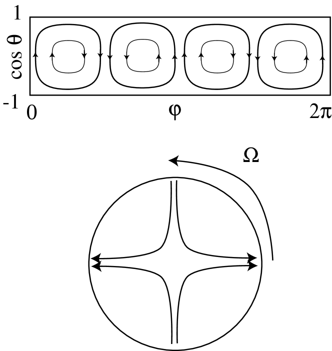
Fig. 9: Schematic illustration of the fluid flow-lines for the lowest order r-mode perturbation relative to the star’s rotation. The arrow indicate the relative direction of fluid flow on adjacent flow-lines. In the upper panel the stars surface (co-latitude $\theta$, longitude $\phi$) is mapped to the plane; in the lower panel, the view is looking down along the stars rotation axis. In both cases, the flow pattern is dragged along by the star’s rotation. At low rotation there is essentially no radial component to the fluids motion; so, we show only the angular components.

In the absence of rotation, the fluid in the star can circulate in the pattern shown with constant velocity: i.e., there are no restoring forces acting on the fluids inertia and the eigenfrequency of the mode is zero. Correspondingly, the magnetic quadrupole moment of this fluid mode has constant amplitude. Rotation introduces Coriolis forces, which act back on the fluid’s inertia and cause the circulation in these cells to be periodic. The quadrupole moment of the fluid momentum now has a second time derivative; correspondingly, it radiates gravitationally.

The power radiated gravitationally comes, ultimately, from the star’s rotational energy. The radiation thus carries off positive angular momentum from the star. The greatest angular momentum can be carried by the modes with azimuthal quantum number $m$ equal to $\pm\ell$; so, focus attention on these modes. Relative to the stars rotation, one of these modes is co-rotating and carries positive angular momentum and one is counter-rotating and carries negative angular momentum. It turns out, however, that both of these modes are dragged, by the stars overall rotation, so that viewed from an inertial frame both carry positive angular momentum. The back-reaction of the radiation adds negative angular momentum to each of these modes; correspondingly, the co-rotating mode is damped and the counter-rotating mode is anti-damped: i.e., it grows. As it grows, of course, it radiates more strongly, leading to greater anti-damping: the mode undergoes exponential growth.

This general mechanism by which gravitational radiation reaction can lead to amplification of a mode that is counter-rotating in the body frame but co-rotating in the inertial frame was first discussed by Zel’dovich in the context of rotating black holes. His concern was that, through this mechanism, a rotating black hole should radiate — a result that anticipated the more general result of Hawking. The first application to stars came from Chandrasekhar [79] and Friedman and Schutz[80] whose focus, however, was on a different set of modes.

Viscosity damps the R-modes. If the viscosity is large enough, then the viscous damping exceeds the anti-damping caused by radiation reaction and the mode is stabilized. Present understanding of the viscosity of neutron star fluid suggests that there is a short period in the life of a new-born neutron star, lasting perhaps one year, when the mode may be unstable and a rapidly rotating star may be a strong, nearly periodic source of gravitational radiation. The radiation is “nearly” periodic because its amplitude is so great that, over the course of the year, the stars angular rotation rate may evolve from $10^{3}$ to $10^{2}$ Hz, simply due to the angular momentum carried away in the radiation[81, 82].

5.3 Stochastic Gravitational Radiation

In the previous subsections we discussed burst and periodic sources of gravitational radiation. In both cases the discussion focused on the source and the radiation was characterized typically in terms of a waveform $h(t)$, which depends on the details of a source and its orientation with respect to the detector.

The situation for a stochastic gravitational wave signal is different. A stochastic gravitational wave signal is intrinsically random in character. In particular, it is not generated by an isolated source, it is not incident on the detector from a single direction, and it has no characteristic waveform.

In fact, a stochastic signal can be treated as just another source of detector noise. The stochastic radiation has an $h(t)$ that is characterized solely by its correlation functions or associated spectra; correspondingly, the detector output owing to the stochastic signal is characterized in terms of correlation functions or associated spectra.

Detection of any signal hinges on observing some characteristic that distinguishes signal from noise. If a stochastic signal appears in a detector no different than intrinsic detector noise, how do we make the critical distinction that allows us to say we have detected a signal?

The essential difference between the action of a stochastic signal and intrinsic detector noise is that stochastic radiation incident on two detectors is correlated, and the correlation depends in a completely predictable way on the relative orientation and separation of the detectors. Any gravitational wave signal — stochastic or otherwise — can be resolved into a superposition of plane waves of different frequencies and propagation directions bathing the detectors. A component of the radiation of given frequency and incident direction drives two or more detectors coherently, with a phase delay that depends on the incidence direction, detector separation and radiation wavelength. For components whose wavelength is much larger than the separation between the detector, the phase difference is only weakly dependent on the radiation wavelength or incident direction; so, summed over incident direction there is a strong correlation between the output of the detectors. On the other hand, for radiation components with wavelengths much smaller than the separation between the detectors the phase difference depends strongly on the incident direction and the wavelength; so, summed over incident direction, the correlation between the output of the detectors is weak. Thus, in the presence of a stochastic gravitational wave background the output of two or more detectors should show predictable correlations that depend on their relative separations, relative orientations, and the stochastic signal’s spectrum[83].

When considering sources of detectable stochastic gravitational radiation for ground-based detectors, it is conventional to enumerate the contributions of primordial origin: e.g., radiation arising during an inflationary epoch in the early universe[84], from the decay of a cosmic string network[85], or from a phase transition in the early universe[86, 87, 88]. Less frequently discussed — perhaps because it is so mundane — are the contributions arising from the confusion limit of discrete but unresolved sources: e.g., core-collapse supernovae[18] or binary inspiral. In fact, the contribution at low-frequencies (periods of hours to minutes) to the stochastic signal from unresolved galactic binary systems is expected to be many times greater than the intrinsic detector noise of the proposed space-based interferometric detector LISA [89, 27].

Let’s talk a bit more about how discrete, well-defined sources — whose waveforms may be well known — can superpose to form a stochastic signal of predictable spectrum. (We focus on burst sources here; however, a similar story can be told for periodic ones.[89])

Astrophysical sources of gravitational-wave bursts strong enough to be observed by conceivable detectors are certainly independent events. Setting aside the slow evolution of the source population on cosmological timescales, the number of events whose radiation impinges upon the receiver during any finite length observation is Poisson distributed: if the event rate is $\dot{N}$ and the observation period is $\tau$, then

$$P(n|\tau\dot{N})={\left(\tau\dot{N}\right)^{n}\over n!}e^{-\tau\dot{N}}.$$ (170)

It is critical to recognize that the number of events exciting the detector at any given moment is not the constant equal to the product of the event rate and the signal duration. The actual number of events in the observation period varies. Averaged over many intervals it has a mean value, which is the product of the event rate and the signal duration. For example, table 1 shows the number of Poisson distributed events over consecutive five second intervals, the rate calculated separately in each interval, and the overall average rate.

Interval	# events	“rate”
0–5 s	3	0.6/s	number in
5–10 s	4	0.6/s	any interval
10–15 s	11	0.6/s	varies from
15–20 s	2	0.6/s	long-run rate
20–25 s	5	0.6/s
0–25 s	25	1.0/s	long-run rate

Table 1: Number of Poisson distributed events, with mean rate 1/s, occurring in consecutive five second intervals. Note that the number of events in any given interval varies: the rate is only the mean of the distribution of “rates” calculated over many intervals.

Now let’s suppose that the “events” we are discussing are the arrival at our detector of the initial wavefront associated with an impulsive perturbation of a black hole. That waveform is a damped sinusoid:

$$h(t)\propto e^{-2\pi f(t-t_{0})/Q}\sin 2\pi f(t-t_{0})\qquad\mbox{for $t>t_{0}$.}$$ (171)

The signal from a single, prototypical event is shown in figure 10. The left-hand panels of figure 11, on the other hand, shows $h(t)$ at the detector when signals exactly like these arrive at the detector with different rates. In the top panel the signals are, for the most part, clearly distinguishable. In the middle panel the rate is higher and separate signals can be distinguished only in exceptional cases. In the bottom panel the rate is higher still and the identity of the individual signals is completely obscured.

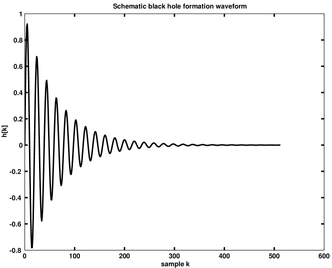
Fig. 10: The prototypical waveform associated with an impulsive perturbation of a black hole: an exponentially damped sinusoid.

Especially in the bottom panel of figure 11, the signal $h(t)$ at any given $t$ is the superposition of a large, but random, number of signals. Similarly, the amplitude of each contributing signal is itself random (corresponding to the signal amplitude at a random moment relative to the signal start time). In circumstances like these we expect The Central Limit Theorem [90] to apply, leading to a normal distribution for $h(t)$. On the other hand, at the lower rate pictured in the top panel, there are not enough events superposed at any given moment for us to expect $h(t)$ to exhibit a normal distribution. In the right-hand panels of figure 11 we show the distribution of $h(t)$ taken from the left-hand panel and find that these intuitions are borne out.

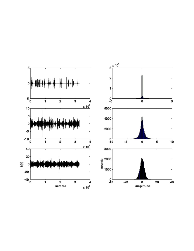
Fig. 11: The left-hand panes show waveforms corresponding to the superposition of many discrete and idealized black hole formation events, with the number of events in a fixed interval Poisson distributed. The rate increases by an order of magnitde from the top to the middle panel, and again from the middle to the bottom panel. The right-hand panes show the distribution of wave amplitude derived from the corresponding left-hand panel.

Note that none of these conclusions depend in any way on the details of the signal from an individual source: instead of the superposition of damped sinusoids we could just as well have constructed $h(t)$ from the superposition of binary inspiral signals in a fixed bandwidth. We do exactly that in figure 12. Note how the distributions of $h(t)$ at high rate are, for superpositions of large numbers of signals, identical (i.e., they are normal distributions).

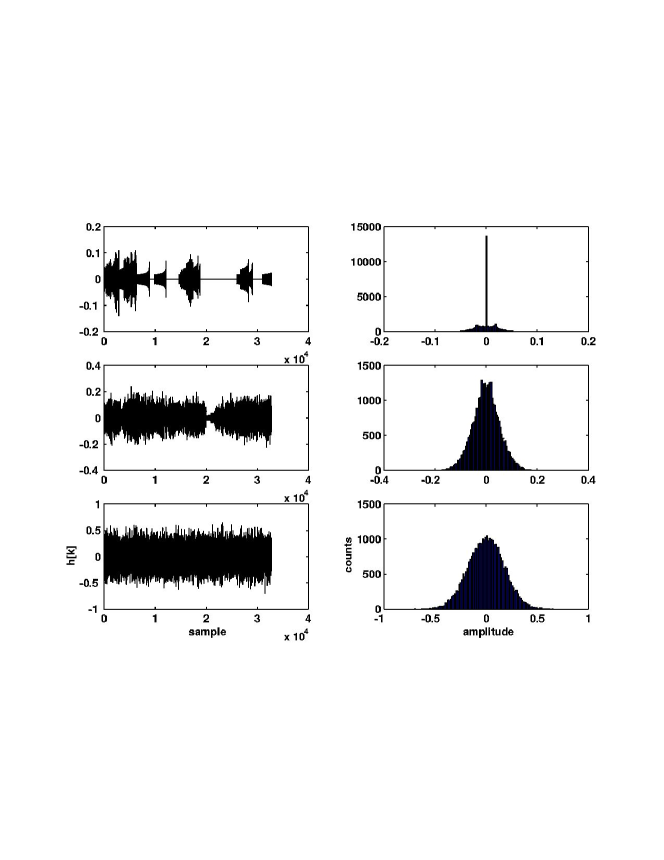
Fig. 12: As in figure 11, but with band-limited binary inspiral waveforms.

Despite the fact that the distribution of $h(t)$ arising from the superposition of a large number of sources are identical, visual inspection suggests that there are still differences. These differences are associated with the correlations: the distribution of the products $h(t)h(t+\tau)$ as a function of $\tau$. These are very different for the damped sinusoids, which are characteristic of black hole perturbations, and the “chirps”, which are characteristic of binary inspiral. In figure 13 we show the power spectral densities of the superpositions in figures 11 and 12. Note how the power spectral densities of the stochastic signals formed from the random superposition of events of a given character preserve the spectral shape of the underlying signal, with the overall amplitude proportional to the event rate. It is this property of the superposition that permits us to predict the character of the stochastic signal arising from the confusion limit of a large number of sources; conversely, observation of a stochastic signal provides us, through its amplitude and spectrum, information about the underlying source, its rate and spatial distribution.

This last point gives us the prospect of using a detected stochastic background, arising from the superposition of unresolved sources, to perform a source “census”: a determination of the density of sources in space. This information, in turn, can shed light on astrophysical process that are otherwise unobservable. An excellent example of this comes from LISA observations of the background from close white dwarf binary systems (CWDBs).[91] These binary systems, which have orbital periods ranging from days to hours, are so close that they are optically unobservable as binaries. We know they exist, nevertheless, because we can see their progenitor systems. CWDBs arise as one of the end-points of binary star evolution, following a particularly difficult to understand and model evolutionary stage where the two stars are orbiting each other within a single envelope of gas. Once they emerge from this final stage of common envelope evolution they orbit each other as if point masses. Gravitational radiation reaction leads to a slow, secular decay in the orbit of these systems until they become so close that mutual tidal interactions lead to rapid orbital decay or stellar disruption.

Let $dn/df$ be the number density of CWDBs with orbital frequency $f$. The amplitude of the stochastic gravitational wave signal from this population of objects is, at frequency $2f$, proportional to $dn/df$. CWDBs are introduced into the population at a rate $d\dot{n}_{+}/df$ as they emerge from the final stage of common envelope evolution at orbital frequency $f$; similarly, they leave the population at a rate $d\dot{n}_{-}/df$ as they disrupt at orbital frequency $f$. Knowing the rate $d\dot{n}_{+}/df$ would provide us valuable information about common envelope evolution, which we cannot obtain through optical observations; similarly, the rate $d\dot{n}_{-}/df$ depends on the white dwarf mass spectrum (we know the white dwarf equation of state quite well) and knowing it would reveal the mass spectrum of binaries emerging from the common envelope evolution stage.

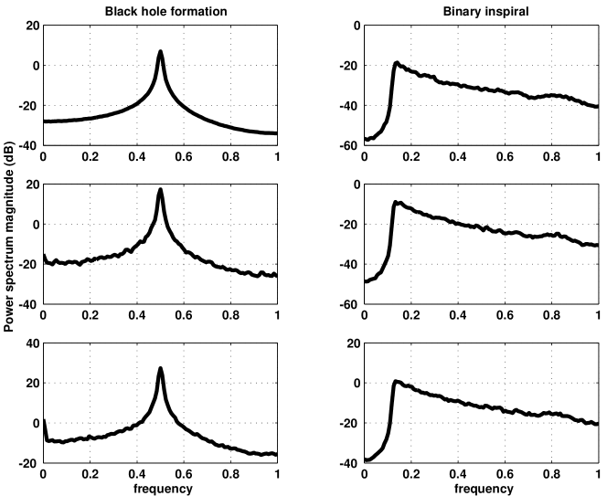
Fig. 13: Power spectra corresponding to the superpositions of black hole ringdown signals in figure 11 and binary inspiral signals in figure 12. The power spectra reflects the underlying source of the stochastic signal (black hole ringdown or binary inspiral) while the amplitude is proportional to the rate of individual sources contributing to the signal.

We can determine both $d\dot{n}_{+}/df$ and $d\dot{n}_{-}/df$ from LISA observation of the CWDB stochastic signal spectrum. Observation of this spectrum determines, as we have seen, $dn/df$. Once injected into the population, a CWDB’s orbit evolves owing exclusively to gravitational radiation reaction, which proceeds at the rate $df/dt$, until it is removed from the population through coalescence or disruption. In steady state we thus have a continuity equation governing the CWDB population:

$${d\dot{n}_{+}\over df}-{d\dot{n}_{-}\over df} = {d\over df}\left({dn\over df}{df\over dt}\right).$$ (172)

The orbital frequency evolution rate $df/dt$ is known (it is proportional to $f^{11/3}$) and LISA observations will determine the number density $dn/df$; consequently, from LISA observations we can determine $d\dot{n}_{+}/df$ and $d\dot{n}_{-}/df$ and learn about the end of common envelope evolution and the mass spectrum of white dwarfs in CWDBs.

6 Conclusions

In these lectures I’ve tried to give a brief overview of how we think about gravitational waves when we set out to detect them, and provide a snapshot of current thinking on the anticipated wave sources. Along the way, I’ve tried to describe some of the science we can hope to do once we can reliably detect gravitational wave sources.

The principal difficulty in discussing the sources that we hope to observe is our real lack of knowledge of their character. As is often the case, however, this difficulty is really a disguised opportunity: when the detectors come on-line and we begin to detect gravitational radiation sources, we will not simply be confirming what we already know, but learning things entirely new about the cosmos!

References

- [1] J. H. Taylor and J. M. Weisberg. A new test of general relativity: gravitational radiation and the binary pulsar PSR 191316. Astrophys. J., 253:908–920, 1982.
- [2] J. H. Taylor and J. M. Weisberg. Further experimental tests of relativistic gravity using the binary pulsar PSR 191316. Astrophys. J., 345:434–450, October 1989.
- [3] S. D. Mohanty, Lee Samuel Finn, and Joseph Romano. Detecting and association between gamma-ray and gravitational wave bursts.
- [4] Steven Weinberg. Gravitation and Cosmology: Principles and Applications of the General Theory of Relativity. Wiley, New York, 1972.
- [5] C. W. Misner, K. S. Thorne, and J. A. Wheeler. Gravitation. Freeman, San Francisco, 1973.
- [6] Bernard F. Schutz. A first course in general relativity. Cambridge University Press, 1990.
- [7] Hans Stephani. General Relativity. Cambridge University Press, Cambridge, second edition, 1993.
- [8] Hans C. Ohanian and Remo Ruffini. Gravitational and Spacetime. Norton, New York, second edition, 1994.
- [9] Kip S. Thorne. Multipole expansions of gravitational radiation. RMP, 52(2):299–339, April 1980.
- [10] John David Jackson. Classical Electrodynamics. Wiley, New York, second edition, 1975.
- [11] Lee Samuel Finn. Gravitational waves from solar oscillations: Proposal for a transition-zone test of general relativity. cqg, 2:381–402, 1985.
- [12] Stuart L. Shapiro and Saul A. Teukolsky. Black Holes, White Dwarfs, and Neutron Stars. Wiley, New York, 1983.
- [13] Thomas Zwerger and Ewald Müller. Gravitational radiation from rotational core collapse. http://www.mpa-garching.mpg.de/ ewald/GRAV/grav.html, 1998.
- [14] Warren W. Johnson and Stephen M. Merkowitz. Truncated icosahedral gravitational wave antenna. PRL, 70(16):2367–2370, 19 April 1993.
- [15] W. O. Hamilton, Ziniu K. Geng, Warren W. Johnson, Evan Mauceli, Stephen M. Merkowitz, Andrew Morse, and Norert Solomonson. Performance of the ALLEGRO detector — and what our experience tells us about spherical detectors. In Jr. et al. [22], pages 19–26.
- [16] E. Mauceli, Z. K. Geng, W. O. Hamilton, W. W. Johnson, S. Merkowitz, A. Morse, B. Price, and N. Solomonson. The allegro gravitational wave detector: Data acquistion and analysis. Phys. Rev. D, 54:1264, 1996.
- [17] P. Astone, M. Bassan, P. Bonifazi, P. Carelli, E. Coccia, C. Cosmelli, V. Fafone, S. Frasca, A. Marini, G. Mazzitelli, Y. Minekov, I. modena, G. Modestino, A. Moleti, G. V. Pallotino, M. A. Papa, G. Pizzella, P. Rapagani, F. Ricci, F. Ronga, R. Terenzi, M. Visco, and L. Votano. The gravitational wave detectors EXPLORER and NAUTILUS. In Jr. et al. [22], pages 39–50.
- [18] D. Blair and L. Ju. A cosmological background of gravitaitonal waves produced by supernovae in the early Universe. Mon. Not. R. Astron. Soc., 283:648–650, 1996.
- [19] Stephen M. Merkowitz and Warren W. Johnson. Spherical gravitational wave antennas and the truncated icosahedral arrangements. PRD, 51(6):2546–2558, 15 March 1995.
- [20] Stephen M. Merkowitz and Warren W. Johnson. First tests of a truncated icosahedral gravitational wave antenna. PRD, 53(10):5377–5381, 15 May 1996.
- [21] G. Frossati. A 100 TON 10mK spherical gravitational wave detector. In Jr. et al. [22], pages 163–168.
- [22] W. F. Velloso Jr., O. D. Aguiar, and N. S. Magalhaes, editors. Omnidirectional Gravitational Radiation Observatory, Singapore, 1997. World Scientific.
- [23] C. Bradaschia, R. del Fabbro, A. di Virgilio, A. Giazotto, H. Kautzky, V. Montelatici, D. Passuello, A. Brillet, O. Cregut, P. Hello, C. N. Man, P. T. Manh, A. Marraud, D. Shoemaker, J. Y. Vinet, F. Barone, L. Di Fiore, L. Milano, G. Russo, J. M. Aguirregabiria, H. Bel, J. P. Duruisseau, G. Le Denmat, Ph. Tourrenc, M. Capozzi, M. Longo, M. Lops, I. Pinto, G. Rotoli, T. Damour, S. Bonazzola, J. A. Marck, Y. Gourghoulon, L. E. Holloway, F. Fuligni, V. Iafolla, and G. Natale. The VIRGO project - a wide band antenna for gravitational-wave detection. Nucl. Instrum. Methods Phys. Research, A289:518–525, 1990.
- [24] Alex Abramovici, William E. Althouse, Ronald W. P. Drever, Yekta Gürsel, Seiji Kawamura, Fredrick J. Raab, David Shoemaker, Lisa Sievers, Robert E. Spero, Kip S. Thorne, Rochus E. Vogt, Rainer Weiss, Stanley E. Whitcomb, and Michael E. Zucker. LIGO: The laser interferometer gravitational-wave observatory. Science, 256:325–333, April 1992.
- [25] Karsten Danzmann. The GEO project: A long baseline laser interferometer for the detection of gravitational waves. Lecture Notes in Physics, 410:184–209, 1992.
- [26] P. Bender, I. Ciufolini, K. Danzmann, W. Folkner, J. Hough, D. Robertson, A. Rüdiger, M. Sanford, R. Schilling, B. Schutz, R. Stebbins, T. Sumner, P. Touboul, S. Vitale, H. Ward, W. Winkler, J. Cornelisse, F. Hechler, Y. Jafry, and R. Reinhanrd. LISA. Laser Interferometer Space Antenna for the detecion and observaiton of gravitational waves. Max-Planck-Institut für Quantenoptik, Hans-Kopfermann-Str. 10, D-85748 Garching, February 1996. MPQ 208.
- [27] William M. Folkner, editor. Laser Interferometer Space Antenna, number 456 in AIP Conference Proceedings, Woodbury, New York, July 1998. American Institute of Physics.
- [28] P.R. Saulson. How an interferometer extracts and amplifies power from a gravitational wave. Class. Quant. Grav, 14:2435–2454, 1997.
- [29] Lee Samuel Finn. Detection, measurement, and gravitational radiation. Phys. Rev. D, 46(12):5236–5249, 1992.
- [30] Peter R. Saulson. Thermal noise in mechanical experiments. PRD, 42(8):2437–2445, 1990.
- [31] Lee Samuel Finn. Gravitational-wave data analysis with multiple detectors: The gravitational-wave receiver. I. Deterministic signals. In preparation.
- [32] Lee Samuel Finn. Science benchmarks for LIGO. Technical Report T970167, California Institute of Technology, LIGO Laboratory, California Institute of Technology, Pasadena CA 91125, September 1997.
- [33] Lawrence E. Kidder, Clifford M. Will, and Alan G. Wiseman. Innermost stable orbits for coalescing binary systems of compact objects. cqg, 9:L125–L131, 1992.
- [34] Lars Bildsten and Curt Cutler. Tidal interactions of inspiraling compact binaries. Astrophys. J., 400:175–180, November 1992.
- [35] Wynn C. G. Ho and Dong Lai. Resonant tidal excitations of rotating neutron stars in coalescing binaries. astro-ph/9812116, December 1998.
- [36] Luc Blanchet, Guillaume Faye, and Bénédicte Posnot. Gravitational field and equations of motion of compact binaries to 5/2 post-Newtonian order. Phys. Rev. D, 58, 1998.
- [37] Luc Blanchet, Thibault Damour, Bala R. Iyer, Clifford M. Will, and Alan G. Wiseman. Gravitational-radiation damping of compact binary systems to second post-Newtonian order. Phys. Rev. Lett., 74(18):3515–3518, 1 May 1995.
- [38] Lee Samuel Finn and David F. Chernoff. Observing binary inspiral in gravitational radiation: One interferometer. Phys. Rev. D, 47(6):2198–2219, 1993.
- [39] Lee Samuel Finn. Binary inspiral, gravitational radiation, and cosmology. Phys. Rev. D, 53(6):2878–2894, 15 March 1996.
- [40] I. H. Stairs, Z. Arzoumanian, F. Camilo, A. G. Lyne, D. J. Nice, J. H. Taylor, S. E. Thorsett, and A. Wolszczan. Measurement of relativistic orbital decay in the PSR B153412 binary system. Astrophys. J., 505:352, 1998.
- [41] Hans A. Bethe and G. E. Brown. Evolution of binary compact objects which merge. Astrophys. J., 506:780, 1998.
- [42] Hans A. Bethe and G. E. Brown. Contribution of high-mass black holes to mergers of compact binaries. astro-ph/9805355, May 1998.
- [43] Phillippe Bagot, Simon F. Portegies Zwart, and Lev R. Yungelson. Gamma-ray bursts and density evolution of neutron star binary mergers. astro-ph/9802094, February 1998.
- [44] Lev Yungelson and Simon F. Portegies Zwart. Evolution of close binaries: Formation and merger of neutron star binaries. astro-ph/9801127, January 1998.
- [45] Ramesh Narayan, Tsvi Piran, and A. Shemi. Neutron-star and black hole binaries in the galaxy. APJL, 379:L17–L20, 1991.
- [46] E. Sterl Phinney. The rate of neutron star binary mergers in the universe: Minimal predictions for gravity wave detectors. Astrophys. J., 380(1):L17–L21, 1991.
- [47] Lee Samuel Finn. A numerical approach to binary black hole coalescence. In M. Francavigli, G. Longhi, L. Lusanna, and E. Sorace, editors, Proceedings of the 14th International Conference on General Relativity and Gravitation, pages 147–166, Singapore, 1997. International Society on General Relativity and Gravitation, World Scientific.
- [48] L. Smarr. Gauge conditions, radiation formulae, and the two black hole collision. In Larry L. Smarr, editor, Sources of Gravitational Radiation, pages 245–274. Cambridge University Press, Cambridge, 1979.
- [49] Peter Anninos, David Hobill, Edward Seidel, Larry Smarr, and Wai-Mo Suen. Collision of two black holes. Phys. Rev. Lett., 71(18):2851–2854, November 1993.
- [50] Peter Anninos, David Hobill, Edward Seidel, Larry Smarr, and Wai-Mo Suen. The head-on collision of two equal mass black holes. Phys. Rev. D, 52:2044–2058, 1995.
- [51] John Baker, Andrew Abrahams, Peter Anninos, Steve Brandt, Richard Price, Jorge Pullin, and Edward Seidel. The collision of boosted black holes. Phys. Rev. D, 55:829, 1997.
- [52] Peter Anninos and Steven Brandt. Head-on collision of two unequal mass black holes. Phys. Rev. Lett., 81:508–511, 1998.
- [53] Gaurav Khanna, John Baker, reinaldo J. Gleiser, Pablo Laguna, Carlos O. Nicasio, Hans-Peter Nollert, Richard Price, and Jorge Pullin. Inspiralling black holes: the close limit, January 1999. Submitted to Science; Center for Gravitational Physics and Geometry Preprint CGPG-99/3-1.
- [54] Éanna É. Flanagan and Scott A. Hughes. Measuring gravitational waves from binary black hole coalescences. I. Signal to noise for inspiral, merger, and ringdown. Phys. Rev. D, 57:4535, 15 April 1998.
- [55] Eanna E. Flanagan and Scott A. Hughes. Measuring gravitational waves from binary black hole coalescences. II. The waves’ information and its extraction, with and without templates. Phys. Rev. D, 57:4566, 15 April 1998.
- [56] Richard H. Price and Jorge Pullin. Colliding black holes: the close limit. PRL, 72(21):3297–3300, 23 May 1994.
- [57] P. Anninos, R. H. Price, J. Pullin, E. Seidel, and W.-M. Suen. Head-on collision of two black holes: Comparison of different approaches. Phys. Rev. D, 52:4462–4480, 1995.
- [58] A. M. Abrahams and R. H. Price. Black-hole collisions from brill-lindquist initial data: Predictions of perturbation theory. Phys. Rev. D, 53:1972–1976, 1996.
- [59] A. M. Abrahams and R. H. Price. Applying black hole perturbation theory to numerically generated spacetime. Phys. Rev. D, 53:1963–1971, 1996.
- [60] Zeferino Andradea and Richard H. Price. Head-on collisions of unequal mass black holes: close limit predictions. Phys. Rev. D, 56:6336, 1997.
- [61] Reinaldo Gleiser, Oscar Nicasio, Richard Price, and Jorge Pullin. The collision of boosted black holes: second order close limit calculations. gr-qc/9802063, February 1998.
- [62] Fernando Echeverria. Phys. Rev. D, 40:3194, 1989.
- [63] Lee Samuel Finn. Detectability of gravitational radiation from supernovae. In J. R. Buchler, S. L. Detweiler, and J. Ipser, editors, Nonlinear Problems in Relativity and Cosmology, pages 156–172. New York Academy of Sciences, New York, 1991.
- [64] Ewald Müller. Gravitational radiation from collapsing rotating stellar cores. Astron. Astrophys., 114:53, 1982.
- [65] Lee Samuel Finn. Gravitational radiation from rotating stellar core collapse. In B. F. Schutz, editor, Gravitational Radiation Data Analysis, pages 33–54. Kluwer, Dordrecht, 1989.
- [66] Lee Samuel Finn and Charles R. Evans. Determining gravitational radiation from Newtonian self-gravitating systems. Astrophys. J., 351:588–600, 1990.
- [67] R. Mönchmeyer, G. Schäfer, E. Müller, and R. E. Kates. AA, 256:417, 1991.
- [68] R. A. Saenz and S. L. Shapiro. Gravitational radiation from stellar collapse - ellipsoidal models. Astrophys. J., 221:286, April 1978.
- [69] R. A. Saenz and S. L. Shapiro. Gravitational and neutrino radiation from stellar core collapse. improved ellipsoidal model calculations. Astrophys. J., 229:286, May 1979.
- [70] R. A. Saenz and S. L. Shapiro. Gravitational radiation from stellar core collapse. III - Damped ellipsoidal oscillations. Astrophys. J., 244:1033, March 1981.
- [71] Lee Samuel Finn. Gravitational radiation sources for acoustic detectors. In Jr. et al. [22], pages 3–12.
- [72] Adam Burrows and John Hayes. Pulsar recoil and gravitational radiation due to asymmetrical stellar collapse and explosion. Phys. Rev. Lett., 76(3):352–355, 15 January 1996.
- [73] A. M. Alpar and David Pines. Gravitational radiation from a solid-crust neutron star. Nature (London), 314:334, 1985.
- [74] Patrick R. Brady, Teviet Creighton, Curt Cutler, and Bernard F. Schutz. Searching for periodic sources with ligo. Phys. Rev. D, D57, 2101-2116 1998.
- [75] Mark Zimmerman and Eugene Szednits. PRD, 20:351, 1979.
- [76] Lars Bildsten. Gravitational radiation and rotation of accreting neutron stars. Astrophys. J. Lett., 501:89, July 1998.
- [77] Nils Andersson. A new class of unstable modes for rotating relativistic stars. Astrophys. J., 502:708, 1998.
- [78] Nils Andersson, Kostas D. Kokkotas, and Nikolaos Stergioulas. On the relevance of the R-mode instability for accreting neutron stars and white dwarfs. astro-ph/9806089, June 1998. To appear in The Astrophysical Journal.
- [79] S. Chandrasekhar. Phys. Rev. Lett., 24:611, 1970.
- [80] J. Friedman and B. F. Schutz. Secular instability of rotating Newtonian stars. Astrophys. J., 222:281–296, 15 May 1978.
- [81] Lee Lindblom, Benjamin J. Owen, and Sharon M. Morsink. Gravitational radiation instability in hot young neutron stars. Phys. Rev. Lett., 80(22), 1 June 1998.
- [82] Benjamin J. Owen, Lee Lindblom, Curt Cutler, Bernard F. Schutz, Alberto Vecchio, and Nils Andersson. Gravitational waves from hot young rapidly rotating neutron stars. Phys. Rev. D, 58, 1998.
- [83] Eanna E. Flanagan. Sensitivity of the Laser Interferometer Gravitational Wave Observatory to a stochastic background, and its dependence on the detector orientations. Phys. Rev. D, 48(6):2389–2407, 15 September 1993.
- [84] Edward W. Kolb and Michael S. Turner. The Early Universe, volume 69 of Frontiers in Physics. Addison-Wesley, Reading, Massachusetts, paperback edition edition, 1994.
- [85] A. Vilenkin and S. Shellard. Cosmic Strings and Other Topological Defects. Cambridge University Press, Cambridge, 1995.
- [86] Marc Kamionkowski, Arthur Kosowsky, and Michael S. Turner. Gravitational radiation from first-order phase transitions. Phys. Rev. D, 49:2837–2851, 15 March 1994.
- [87] Arthur Kosowsky, Michael S. Turner, and Richard Watkins. Gravitational radiation from colliding vacuum bubbles. Phys. Rev. D, 45(12):4514–4535, 15 June 1992.
- [88] Arthur Kosowsky and Michael S. Turner. Gravitational radiation from colliding vacuum bubbles: Envelope approximation to many-bubble collisions. Phys. Rev. D, 47(10):4372–4391, 15 May 1993.
- [89] D. Hils, P. L. Bender, and R. F. Webbink. Astrophys. J., 360:75, 1990.
- [90] Jon Mathews and R. L. Walker. Mathematical Methods of Physics. Benjamin/Cummings, Menlo Park, California, second edition, 1970.
- [91] Lee Samuel Finn. Gravitational Wave Astronomy. In S. Dhurandhar and T. Padmanabhan, editors, Gravitation and Cosmology, pages 95–110, Netherlands, 1997. Kluwer.