Canonical “Loop” Quantum Gravity and Spin Foam Models

Abstract

The canonical “loop” formulation of quantum gravity is a mathematically well defined, background independent, non perturbative standard quantization of Einstein’s theory of General Relativity. Some among the most meaningful results of the theory are: 1) the complete calculation of the spectrum of geometric quantities like the area and the volume and the consequent physical predictions about the structure of the space-time at the Planck scale; 2) a microscopical derivation of the Bekenstein-Hawking black-hole entropy formula. Unfortunately, despite recent results, the dynamical aspect of the theory (imposition of the Wheller-De Witt constraint) remains elusive.

After a short description of the basic ideas and the main results of loop quantum gravity we show in which sence the exponential of the super Hamiltonian constraint leads to the concept of spin foam and to a four dimensional formulation of the theory. Moreover, we show that some topological field theories as the BF theory in 3 and 4 dimension admits a spin foam formulation. We argue that the spin-foams/spin-networks formalism it is the natural framework to discuss loop quantum gravity and topological field theory.

1 Introduction

The loop approach to quantum gravity [RS88, RS90] has reached a mature status as a physical theory and it is one of the most likely candidate to be a complete consistent quantum theory of gravitational phenomena (for a detailed review and update bibliography we refer to [Rov98c] for quantum gravity in general and to [Rov98a] for the loop approach in particular). In this approach it was possible: i) to construct the auxiliary Hilbert space [AI92, AL95] appropriate to the discussion of the kinematics ii) to find an explicit basis (the spin-networks basis) on this Hilbert space [Bae94, RS95b]; iii) to rigorously solve the 3-diffeomorphism constraints [ALM⁺95]; iv) to construct operators corresponding to volume and area and determine their spectrum [RS95a, DR96, AL97, AL98]. v) to derive the Beckenstein-Hawking formula for the entropy of Black Holes [Rov96, BCR96, Kra97, ABCK98]

The elusive feature of the loop approach to quantum gravity is that in the frozen-time canonical picture the relation between operator and physical observable is cumbersome. A space time picture was lacking until M. Reisenberger a C. Rovelli [RR97] derived a spin foam model (using the terminology introduced by J. Baez [Bae98]), to which they refer as world sheet model, from the Exponential of the super-Hamiltonian constraint. They also show that this is formally related to the construction of the 4 dimensional path integral for gravity. This work was a first step in the direction of developing a sum over surfaces framework in “loop quantum gravity” whoose importance was first claimed by Reisenberger in [Rei94]. This recent developments showed surprising formal analogy between loop quantum gravity and other approaches to the quantization of gravity. The model of dynamical triangulation [ACM97] and the Ponzano-Regge model [PR68] are exactly models of this kind. The analogy is even deeper if one considers the Ponzano-Regge model [the physicist version of the celebrated Turaev-Viro state sum model for 3-manifold invariant [TV92])] that can be formulated exactly as a sum over branched surfaces with colored graph observables (spin networks) on the boundary.

The previous consideration, together with the fact that the topological BF field theory in 4 dim [Oog92b], [CKY97] (see also [CKS98]) admits an analogous formulation as a spin foam model [in this case,the spin foam dual to a simplicial decomposition (triangulation)], strongly suggest that quantum gravity should be naturally formulated using the language of spin foam models. Now, two explicit proposals for the realization of this idea have been put forward. The first one (by Barret and Crane [BC98]) is related to the discretization of the path integral of the Euclidean Plebanski action [Ple77] (see [DF98, Rei98]) and the second (by M. Reisenberger [Rei97a]) of self dual Euclidean gravity [Rei95]. The last model is the explicit quantization of the lattice model [Rei97b] that has self dual Euclidean gravity as its continuum limit. This research line is deeply connected to the idea of express classical gravity as a deformation (by the imposition of additional Lagrange constraints) of a topological BF field theory 4 dimension. The idea is that [Hor89] topological BF theory, in the context of diff-invariant theory, can play a role analogue to the one of free theory in standard Poincaré invariant quantum fields theories. This idea is at the origin of the systematic proposal for deriving Spin Foam Weight Factors from a Classical Action Principle that has been recently proposed by Freidel and Krasnov [FK98].

The discussion here it is in framework of piecewise linear topology and we refer the reader to [RS72] for details. Intuitively, this setting is equivalent to assume that cells, surfaces and edges that we use to decompose the manifold are finite unions of piecewise analytic sub-manifolds. In particular, a graph is a finite collection of analytic path. This framework as certain advantages and the resulting theory is simpler than the ones in the analytic or in the smooth setting. The utility of the PL setting in loop quantum gravity was first pointed out by Zapata [Zap98, Zap97]. All the topological objects (graph, manifold, cellular decomposition, ….) are assumed orientable. For the Wigner nJ-symbols we adopt the non normalized graphical convention of [KL94, De 97] and we restrict to the case of the group $SU(2)$ and use Penrose’s binor formalism [Pen71]. Most of the formulas remain valid in the quantum group case, but, in this case, factors related to the braiding can appear.

2 Loop Quantum Gravity

Loop quantum gravity is based on the Hamiltonian formulation of classical general relativity in terms of the canonically conjugated variables $\tilde{E}^{a}_{i}(x)$ (densitized triad fields) and $A_{a}^{i}(x)$ (Ashtekar’s connection) [Ash86]. The dynamics is given, as it happens for any diff-invariant theory, only in terms of constraints. In our case:

$$\begin{array}[]{lr}C_{i}(x)={\cal D}_{a}\tilde{E}^{a}_{i}(x)\simeq 0&\mbox{(Gauge constraints)}\\ {\cal H}_{a}(x)=\tilde{E}^{b}_{i}(x)F^{i}_{ab}(x)\simeq 0&\mbox{(Diffeomorphism constraints)}\\ {\cal H}(x)=\frac{\epsilon^{ijk}}{\sqrt{g}}\tilde{E}^{a}_{i}(x)\tilde{E}^{b}_{j}(x)F^{k}_{ab}(x)\simeq 0&\mbox{(Hamiltonian constraints).}\end{array}$$

The loop program does the quantization of gravity in a straightforward way. It is based on the assumption that a particular class of classical functions (the ${\cal T}$ observables, i.e., the traces of the holonomy of Ashtekar’s connection) become well defined quantum operators. I.e., it is assumed that, for any choice of the close loop $\gamma$, to the classical functional of the Ashtekar connection:

$${\cal T}_{\gamma}[A_{a}^{i}(x)]={\rm Tr}\left[\exp\left(\int_{\gamma}A_{a}(x)dx^{a}\right)\right]$$ (1)

corresponds a well defined quantum operator on a Hilbert space ${\cal H}$. All the other properties should be essentialy derived from this assumption. A consequence of this choice is that the canonical variables $\tilde{E}^{a}_{i}(x)$,$A_{a}^{i}(x)$ do not become well defined operator on the Hilbert space ${\cal H}$ and the previous definition of the constraint (unless properly regularized) are meaningless on ${\cal H}$. This is one of the main technical reasons behind the difficulty of dealing with the super-Hamiltonian constraint.

Given this assumption, there are two possible ways to define the theory. Explicitly construct the vector space on which these operators are well defined (loop representations, see [DR96]), in a algebraic way, and then determine the correct scalar product. Alternatively, construct a Hilbert space ${\cal H}$ (the connection representation) and show that, on this Hilbert space, these operators are well defined [ALM⁺95]. These two approaches are equivalent [De 97]. However, two technical but important decision must be taken. The first one is connected to the properties of the loops $\gamma$. The request of piecewise analyticity brings to a different setting with respect to the smooth case since two piecewise analytic loop can have only a finite number of isolated intersection points. The second is that these constraction are well defined only in the case of a real connection. Now, the standard Ashtekar connection is naturaly real only in the case of Euclidean gravity while in the case of Lorentzian gravity is naturally complex and indeed what follows naturally applies only to Euclidean gravity. However, it is important to note that, it is possible to use a real connection in the Lorentzian case too (the Barbero connection [Bar95, Bar96]) at the prize of a more complicated form for the super-Hamiltonian constraint.

2.1 The auxiliary Hilbert space

A full discussion of the kinematical setting is not important here. We refer to [ALM⁺95, De 97] for the technical details and for complete references. For the following discusson it is sufficient to recall the basic structure of the Hibert space ${\cal H}$. Since a connection associates a group element $g_{e_{i}}={\cal P}\exp(-\int_{e_{i}}A)$ to each edge (segment embedded in $M^{3}$) of the graph $\gamma$. It is natural to consider for each graph $\gamma$ the Hilbert space (${\cal H}_{\gamma}=L^{2}[G^{n},d\mu(g)]$) of square integrable function, with respect to the unique normalized Haar measure $d\mu(g)$, on $n$ (the number of edges ${e_{i}}$ in $\gamma$) copies of the group [$G=SU(2)$] $G^{n}$. ${\cal H}$ can be characterized as the projective limit of the previous family of Hilbert spaces ${\cal H}_{\gamma}$ associated to all possible graphs $\gamma$ embedded into $M^{3}$.

Figure 1: The graph $\gamma$, a possible extended-planar projection $\Gamma_{ex}$ and the graphical representation of a spin-network cylindrical function

The gauge invariant Hilbert space ${\cal H}_{\rm aux}$ is the projective limit of the gauge invariant sub-sector of the Hilbert spaces ${\cal H}_{\gamma}$. Moreover, the Peter-Weyl theorem gives us a natural basis in this space of gauge invariant functions $f_{\gamma}(g_{e_{1}},\ldots,g_{e_{n}})$, the spin networks basis:

$$f_{\gamma}(g_{e_{1}},\ldots,g_{e_{n}})=\!\sum_{\vec{\pi},\vec{\iota}}\!f(\gamma,\vec{\pi},\vec{\iota})~{}~{}{\cal T}_{\gamma,\vec{\pi},\vec{\iota}~{}}[A],~{}~{}~{}~{}{\cal T}_{\gamma,\vec{\pi},\vec{\iota}}[A]\stackrel{{\scriptstyle def}}{{=}}\left(\otimes_{i=1}^{\#^{\rm edge}}\pi_{i}(g_{e_{i}})\right)\cdot\left(\otimes_{j=1}^{\#^{\rm vertex}}\iota_{j}\right)$$ (2)

where: (i) $\vec{\pi}=(\pi_{1},\ldots,\pi_{N})$ denotes the labeling of the edges with irreducible representation $\pi_{i}$ of $G$; (ii) $\vec{\iota}=(\iota_{1},\ldots,\iota_{M})$ a labeling of the vertices with invariant contractors $\iota_{j}$ (the intertwining matrices $\iota_{j}$, in each of the vertices $v_{j}$, represents the invariant coupling of the $n_{j}$ representations associated to the $n_{j}$ edges that start or end in $v_{j}$). In the case of loop quantum gravity (where $A_{a}^{i}$ is a $SU(2)$ connection) the vector of the basis (a spin network state) are characterized (see figure 1) by a colored (the irreducible representation of $SU(2)$ are label by the associated spin or by an integer, that we call the color of the representations, that its twice the spin) graph.

2.2 The diffeomorphism invariant state

A rigorous definition of the diffeomorphism invariant Hilbert space can be obtained [ALM⁺95] using the gauge averaging procedure. The essential idea is that on ${\cal H}_{\rm aux}$ there is a natural definition of the action of a diffeomorphism $\phi\in{\rm Diff}$ ($\phi:M\rightarrow M$). In fact, in the spin-networks basis we can associated to each diffeomorphism $\phi$ the operator

$$\hat{U}_{\phi}|S\rangle=\hat{U}_{\phi}|\gamma,\vec{\pi},\vec{\iota}~{}\rangle=|\phi(S)\rangle=|S^{\prime}\rangle=|\phi(\gamma),\vec{\pi},\vec{\iota}~{}\rangle,$$ (3)

where $S^{\prime}=\phi(S)$ is the imagine under $\phi$ of the spin network $S$. At this point one can define the class of spin networks knots $s$ as the equivalence class of spin networks under diffeomorphism, i.e. $S,S^{\prime}\in s$ it it exists a $\phi\in{\rm Diff}$ such that $S^{\prime}=\phi(S)$. In this way, we can define ${\cal H}_{\rm Diff}={\cal H}_{\rm aux}/{\rm Diff}$ with the scalar product:

$$\langle s|s^{\prime}\rangle=N\int[D\phi]\langle S|\hat{U}_{\phi}S^{\prime}\rangle=N\int[D\phi]\langle\phi(S)|S^{\prime}\rangle$$ (4)

where $N$ is an arbitrary, not yet fixed, normalization factor and $S,S^{\prime}\in{\cal H}_{\rm aux}$ are two arbitrary spin networks in the $s$-knot class of $s$ and $s^{\prime}$, respectively. The integration in eq. (4) is meaningful because the scalar product of two spin networks of ${\cal H}_{\rm aux}$ is different from zero only if they have support on the same graph.

In the previous derivation of the Hilbert space ${\cal H}_{\rm Diff}$ we made an implicit assumption on the kind of diffeomorphism that are allowed. Having previously assumed that the loops are in the class of the piecewise analytics ones, it is natural to assume piecewise analytics diffeomorphism. In this case, the quotient space ${\cal H}_{\rm Diff}$ is a separable Hilbert space. This leads directly to the PL framework. We refer to the work of Zapata for the discussion of the subtleties involved [Zap97, Zap98].

2.3 The super-Hamiltonian constraint

In the first presentation of loop quantum gravity [RS88, RS90] was emphasized that loops without intersection, (i.e., spin network states whose graph $\gamma$ with only bivalent vertices) it is automatically in the kernel of the super-Hamiltonian constraint. This gives the knowledge of an infinite dimensional subspace of the physical Hilbert space ${\cal H}_{{\rm Phys}}$. Unfortunately, with the introduction of the volume operator [RS95a], it was realized that all the spin network states based on graph $\gamma$ with all vertices of valence less that $3$ are in the kernel of the volume operator. Consequently, all the previously mentioned states, belonging to the kernel of the super-Hamiltonian constraint, correspond to degenerate metrics and, therefore, can not correspond to genuine quantum 3 geometries. This urged the definition of the super-Hamiltonian constraint ${\cal H}(x)$ on the whole diff-invariant Hilbert space ${\cal H}_{\rm Diff}$.

The situation improved in 1996 when Thiemann [Thi96, Thi98a, Thi98b] was able to construct an operator with the naivë classical limit. Using this definition, it is possibile investigate the true physical Hilbert space ${\cal H}_{{\rm Phys}}$. For the purpose of the present discussion we do not need a complete account of its definition and its properties. What it is interesting for us it is that: 1) it is possible to define such operator; 2) a rough idea of its action ${\cal H}_{\rm Diff}$. Its main property is that it acts locally around each vertex of the spin network. It adds or deletes an edge of color 1

$$\hat{A}_{vIJK\bar{\epsilon}\tilde{\epsilon}}=\left\langle\begin{array}[]{c}\begin{picture}(65.0,50.0)\put(0.0,0.0){\line(1,1){20.0}} \put(0.0,20.0){\line(1,0){20.0}} \put(0.0,40.0){\line(1,-1){20.0}} \put(20.0,20.0){\circle*{3.0}} \put(20.0,20.0){\line(3,2){30.0}} \put(52.0,38.0){$\scriptstyle K$} \put(20.0,20.0){\line(3,-2){30.0}} \put(52.0,2.0){$\scriptstyle J$} \put(45.0,8.0){$\scriptstyle p$} \put(45.0,30.0){$\scriptstyle q$} \put(15.0,2.0){$\scriptstyle p\!+\!\bar{\epsilon}$} \put(15.0,32.0){$\scriptstyle q\!+\!\tilde{\epsilon}$} \put(35.0,10.0){\line(0,1){20.0}} \put(35.0,10.0){\circle*{3.0}} \put(35.0,30.0){\circle*{3.0}} \put(37.0,20.0){$\scriptstyle 1$} \end{picture}\end{array}\right|\hat{\cal H}[N]\left|\begin{array}[]{c}\begin{picture}(65.0,50.0)\put(0.0,0.0){\line(1,1){20.0}} \put(0.0,20.0){\line(1,0){20.0}} \put(0.0,40.0){\line(1,-1){20.0}} \put(20.0,20.0){\circle*{3.0}} \put(20.0,20.0){\line(3,2){30.0}} \put(52.0,38.0){$\scriptstyle K$} \put(20.0,20.0){\line(3,-2){30.0}} \put(52.0,2.0){$\scriptstyle J$} \put(45.0,8.0){$\scriptstyle p$} \put(45.0,30.0){$\scriptstyle q$} \end{picture}\end{array}\right\rangle$$ (5)

with well definite weight factors [($\hat{A}_{vIJK\bar{\epsilon}\tilde{\epsilon}}$) matrix elements of the operator] that can be explicitly computed [BDR97].

2.4 The hierarchy of Hilbert spaces of loop quantum gravity

Summarizing, the mathematical definition of the loop quantization of gravity, and the determination of the physical Hilbert space ${\cal H}_{{\rm Phys}}$, involves the analysis of the following hierarchy of Hilbert spaces:

$${\cal H}~{}\stackrel{{\scriptstyle C_{i}(x)}}{{\Longrightarrow}}~{}{\cal H}_{{\rm aux}}~{}\stackrel{{\scriptstyle{\cal H}_{a}(x)}}{{\Longrightarrow}}~{}{\cal H}_{{\rm Diff}}~{}(?)\!\stackrel{{\scriptstyle{\cal H}(x)}}{{\Longrightarrow}}\!(?)~{}{\cal H}_{{\rm Phys}}$$ (6)

where an arrow means imposition of a constraint and the questions mark emphasis the fact that, the last step, it is still not completely understood. In fact: 1) the physical correctness of the Thiemann’s proposal for the regularization of the super-Hamiltonian constraint has been questioned; 2) more of one variant of this operator can be construct and indeed the problem of determine the correct one; 3) despite [Thi98c] there is not a clear understanding of the kernel of the super-Hamiltonian constraint nor of the class of operator that are well defined on this Hilbert space.

3 The exponential of the Hamiltonian constraint

Reisenberger and Rovelli in [RR97, Rov98b] suggested (taking advance of the existence of a well defined version of the Hamiltonian constraint [Thi96, Thi98a, Thi98b] on ${\cal H}_{{\rm Diff}}$) that the better way to address this last remaining problem is to use a 4-dimensional picture. In the case of classical general relativity the lapse ${N}(x,\tau)$ and shift function $N^{a}(x,\tau)$ ($N^{\mu}(x,\tau)=d\Sigma^{\mu}(x,\tau)/d\tau$) generate the evolution along a foliations ($\Sigma(\tau)$) between $\Sigma(0)$ and $\Sigma(1)$. In an analogous way, in the quantum case, we can say that the lapse and shift function generate the evolution from a spin network state $|s,\Sigma(0)\rangle\in{\cal H}_{\rm aux}$ associated to the boundary $\Sigma(0)$ to the spin network state $|s^{\prime},\Sigma(1)\rangle\in{\cal H}_{\rm aux}$ associated to the boundary $\Sigma(1)$. Formally we have

$$\frac{d}{dt}|S^{\prime},\Sigma(1)\rangle = ~{}\bigg{(}N(x,\tau)\hat{\cal H}(x)+N^{a}(x,\tau)\hat{\cal H}_{a}(x)\bigg{)}|S,\Sigma(t)\rangle$$ (7)

$$|S^{\prime},\Sigma(1)\rangle = {\cal T}\!\!\exp\bigg{[}\!\!-\!{\rm i}\!\int_{0}^{T}\!\!\!d\tau\!\int\!\!d^{3}\!x~{}\bigg{(}N(x,\tau)\hat{\cal H}(x)+N^{a}(x,\tau)\hat{\cal H}_{a}(x)\bigg{)}\bigg{]}|S,\Sigma(0)\rangle~{}~{}.$$ (8)

The last equation suggests to define the transition amplitude, averaged over all the possible embedding (bordism) interpolating from $\Sigma(0)$ and $\Sigma(1)$:

$$Z[S^{\prime},S;1]=\langle S^{\prime},\Sigma(1)|S,\Sigma(0)\rangle=$$ (9)

$$~{}~{}~{}~{}~{}=\int[dN(x,\tau)][dN^{i}(x,\tau)]\langle s^{\prime}|{\cal T}\!\!\exp\bigg{[}\!\!-\!{\rm i}\!\int_{0}^{1}\!\!\!d\tau\!\int\!\!d^{3}\!x~{}\bigg{(}N(x,\tau)\hat{\cal H}(x)+N^{a}(x,\tau)\hat{\cal H}_{a}(x)\bigg{)}\bigg{]}|S\rangle~{}~{}.~{}~{},$$

where the integrations $[dN(x,\tau)][dN^{i}(x,\tau)]$ are over all the lapse and shift functions that represent a bordism between $\Sigma(0)$ and $\Sigma(1)$. They note that it is possible to give a well defined meaning to the integration over the lapse of the exponential of infinitesimal diffeomorphism in term of the gauge averaging procedure used in [ALM⁺95] to solve the diffeomorphism constraints:

$$\hat{U}_{\phi_{N^{i}}} =: \exp\bigg{[}\!\!-\!{\rm i}\int\!d^{3}\!x~{}N^{a}(x)\hat{{\cal H}}_{a}(x)\bigg{]}$$ (10)

$$|s\rangle := \int[D\phi]~{}\hat{U}_{\phi}|S\rangle=:\int[dN^{a}(x)]~{}\hat{U}_{\phi}|S\rangle$$ (11)

and then, using a series of formal argument, that the definition (9) depends only on the s-knot classes $s$ and $s^{\prime}$ of $S$ and $S^{\prime}$, respectively. Morover, they show that it can be expressed in term of a diff-invariant definition (as the one proposed by Thiemann) of the super-Hamiltonian constraint and of its associated proper time propagator:

$$Z_{RR}[s^{\prime},s;1]=\int dT<s^{\prime}|e^{{\textstyle-{\rm i}}~{}T~{}{\cal H}}|s>=\int dT\sum_{\sigma}\frac{({\rm i}~{}T)^{n(\sigma)}}{n(\sigma)}\prod_{({\rm coloring~{}of~{}}\sigma)}\prod_{v\in[\sigma]}A_{v}(\sigma)$$ (12)

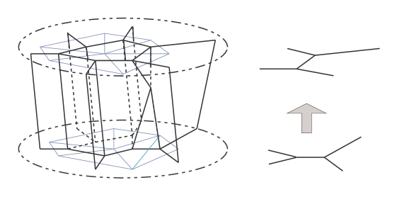
Figure 2: A potential first order contribution to the partition function $Z_{RR}[s^{\prime},s;\sigma;1]$ of eq. (3) and the corresponding spin-network transition. A three dimensional situation is reported. From the point of view of a 4 dimensional theory this contribution correspond to a branched polyhedron dual to a singular triangulation.

In the previous equation, ${\cal H}$ is a diff-invariant definition of the Hamiltonian constraints and $\sigma$ is a 2-dimensional branched surface embedded over $\Sigma\times I[0,T]$. In figure 2 we reported an example of branched surface, and of the corresponding spin-network transition. The kind of surfaces that appear on the sum is explicitly determined by the kind of non null matrix elements of the super-Hamiltonian constraints. We want to emphasize, once more, that this derivation is based on formal argument. The use of formal argument is of great help to understand the general picture behind but one should stop here. The result of this formal derivation is that the functional integral associate to quantum gravity is defined (or, better, should be) as a sum over branched surface interpolating between two spin networks. Moreover, it shows that one has to consider the sum over all the possible (not just one) such branched surfaces. This in a deep breakthrough toward the understanding of loop quantum gravity and it shows a strict relationship between loop quantum gravity and topological field theories of BF type opening the possibility of use technics developed for such theories.

The first occurrence, (to our knowledge) of the idea of formulating the transition amplitude between two Hilbert space (spanned by embedded colored graph) associated to two boundary component of a Manifolds, as a weight associated to the colored branched surface interpolending between the two graphs, first appeared in Turaev and Viro [TV92]. These authors used the terms: two dimensional polyhedral quantum field theory (Spin foam models are model of this kind). The next section will be dedicated to the exposition of this idea in the case of 2+1 dimensional gravity or, more precisely, of the Ponzano-Regge-Turaev-Viro model.

4 The Ponzano-Regge-Turaev-Viro Model

The Ponzano-Regge model and its quantum group analogous, the Turaev-Viro partition function [it is known that its evaluation gives a quantum invariants of 3-manifolds], are the better understood example of theory formulated on a triangulation $\Delta$ of a manifold $M$. From the physical point of view it is known (for details see [OS91, Oog92a, AW91]) that it correspond to the quantization of Euclidean 2+1 dimensional gravity, i.e., to the quantization of the $SU(2)$ BF theory in 3 dimension:

$$Z_{BF}^{(3)} = \int[{\cal D}e(x)][{\cal D}\omega(x)]e^{{\rm i}\int{\rm Tr}[e\wedge R[\omega]]+\Lambda~{}{\rm Tr}[e\wedge e\wedge e]}$$

$$= \int[{\cal D}A(x)][{\cal D}B(x)]e^{\frac{{\rm i}k}{4\pi}\int[{\rm Tr}[A\wedge F[A]]+\frac{2}{3}{\rm Tr}[A\wedge A\wedge A]]-[{\rm Tr}[B\wedge F[B]]+\frac{2}{3}{\rm Tr}[B\wedge B\wedge B]]}$$

$$= \left|\int[{\cal D}A(x)]e^{\frac{{\rm i}k}{4\pi}\int+{\rm Tr}[A\wedge F[A]]+\frac{2}{3}{\rm Tr}[A\wedge A\wedge A]}\right|^{2}=|Z_{CS}|^{2}$$

where

$$\omega=\frac{1}{2}\left[A+B\right]~{}~{}~{}~{}~{}~{}~{}~{}e=\frac{k}{8\pi}\left[A-B\right]~{}~{}~{}~{}~{}~{}~{}~{}\Lambda=\left(\frac{4\pi}{k}\right)^{2}$$

The receipt for the construction of this model (to which we will refer to as the PRTV-model) is the following. Color all the edge (1-dimensional object of the triangulation) with irreducible representations of the $SU(2)$ group and assign the following factor to the various object of the triangulation: 1) to each edge the dimension of the representation $\Delta_{c_{e}}$; 2) to each triangle the inverse of the 3J symbol made out by the three colors associated to each of its edges $\theta(a_{t},b_{t},c_{t})^{-1}$; 3) to each tetrahedron the associated 6J symbol (a tetrahedron has 6 edges) ${\rm Tet}[abed;cf]$.

 

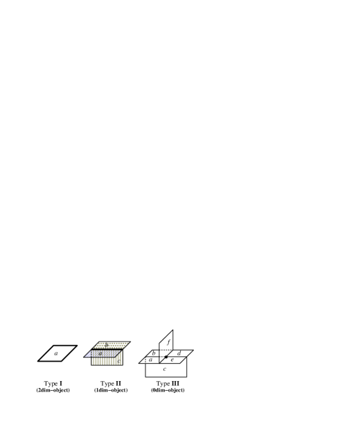
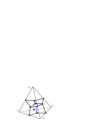
Figure 3: The local description of the standard polyhedron dual to a triangulation and a schematic representation of the duality. Note that in 3 dimension, a coloration of the edges of the triangulation determine a unique coloration of the faces of its dual 2-skeleton, and vice versa.

In the case of the PRTV-model, it is useful to consider its dual formulation, i.e. to take advantage of the duality between triangulation and standard polyhedron suggested by figure 3. In the dual cellular complex $\Delta^{*}$ of the triangulation $\Delta$ we have that to each $n$-dimensional cell of $\Delta$ is uniquely assigned a 3-$n$-dimensional cell of $\Delta^{*}$. In three dimension, the objects dual to an edge (1 dimensional object) is a surface (2=3-1 dimensional object). This implies that to each coloration of the edges of the triangulation $\Delta$ is associated a unique coloration of the face (two dimensional objects) of its dual standard polyhedron $\Delta^{*}$. In turns, it is possible to consider the PRTV-model as a model defined over a two dimensional branched surface. I.e., using this duality, we can interpret the PRTV model both as a state sum model associated to a triangulation but also has a state sum model associated to a branched surface:

$$TV_{G}[M^{3},\Delta]=TV_{G}[{\cal S}_{2}^{\Delta^{*}}]$$ (14)

where by ${\cal S}_{2}^{\Delta^{*}}$ we denote the collection of all the faces, edges and vertices (the 2-scheleton) of the cellular decomposition of $M$ dual to triangulation $\Delta$. We will also use the notations ${\cal F}({\cal S}_{2})$, ${\cal E}({\cal S}_{2})$ and ${\cal V}({\cal S}_{2})$ to denote the collection of its faces, edges and vertices, respectively.

This express the fact that the definition of the PRTV-model can be given as a series of rules with respect to the objects of the triangulation or as an equivalent set of rules with respect to the objects to its dual standard polyhedron:

$\Delta$	$\Delta^{*}$			Factor in $TV[M^{3},\Delta]=TV_{G}[{\cal S}_{2}(\Delta^{*})]$
vertex	3-cell	Type 0		$\Lambda^{-1}=\left[\sum_{a}\Delta_{a}\right]^{(-1)}$
edge	face	Type I		$\Delta_{a}=dim(a)={\!\begin{array}[]{c}\begin{picture}(35.0,25.0)\put(15.0,0.0){\line(0,1){10.0}} \put(20.0,0.0){\line(0,1){10.0}} \put(15.0,0.0){\line(1,0){5.0}} \put(15.0,10.0){\line(1,0){5.0}} \put(15.0,25.0){\line(1,0){5.0}} \put(15.0,15.0){$\scriptstyle{a}$} \put(15.0,15.0){\oval(20.0,20.0)[l]}\put(20.0,15.0){\oval(30.0,20.0)[r]} \end{picture}\end{array}\!}$
face	edge	Type II		$\theta(a,b,c)^{-1}=\left[{{\begin{array}[]{c}\begin{picture}(40.0,40.0)\put(18.0,32.0){$\scriptstyle{a}$} \put(0.0,15.0){\line(1,0){40.0}} \put(18.0,17.0){$\scriptstyle{b}$} \put(20.0,15.0){\oval(40.0,30.0)} \put(18.0,2.0){$\scriptstyle{c}$} \put(0.0,15.0){\circle*{3.0}} \put(40.0,15.0){\circle*{3.0}} \end{picture}\end{array}}}\right]^{(-1)}$
tetrahedron	vertex	Type III		${\rm Tet}[{abed};{cf}]={\begin{array}[]{c}\begin{picture}(50.0,30.0)\put(0.0,15.0){\line(1,-1){15.0}} \put(0.0,22.0){${\scriptstyle{b}}$} \put(0.0,15.0){\line(1,1){15.0}} \put(0.0,0.0){${\scriptstyle{a}}$} \put(0.0,15.0){\circle*{3.0}} \put(30.0,15.0){\line(-1,1){15.0}} \put(28.0,20.0){${\scriptstyle{e}}$} \put(30.0,15.0){\line(-1,-1){15.0}} \put(28.0,2.0){${\scriptstyle{d}}$} \put(30.0,15.0){\circle*{3.0}} \put(0.0,15.0){\line(1,0){30.0}} \put(12.0,16.0){${\scriptstyle{c}}$} \put(15.0,30.0){\line(1,0){25.0}} \put(15.0,30.0){\circle*{3.0}} \put(15.0,0.0){\line(1,0){25.0}} \put(15.0,0.0){\circle*{3.0}} \put(40.0,0.0){\line(0,1){30.0}} \put(42.0,12.0){${\scriptstyle{f}}$} \end{picture}\end{array}}$

One of the nice characteristic of the dual formulation is that it involves only the coloring of a 2-dimensional standard polyhedron embedded into the Manifold. Completing the transition to the dual world it is possible to to forget the original triangulation and to directly associate a state-sum to any standard polyhedron of the ($M^{3}$) manifold.

$$TV_{G}[{\cal S}_{2}]=\Lambda^{\scriptscriptstyle-\#(3-cells)}\!\!\!\!\!\sum_{\vec{c}\in D({\cal S}_{2},G)}\left[\!\prod_{f\in{\cal F}({\cal S}_{2})}\!\left({\!\begin{array}[]{c}\begin{picture}(35.0,25.0)\put(15.0,0.0){\line(0,1){10.0}} \put(20.0,0.0){\line(0,1){10.0}} \put(15.0,0.0){\line(1,0){5.0}} \put(15.0,10.0){\line(1,0){5.0}} \put(15.0,25.0){\line(1,0){5.0}} \put(15.0,15.0){$\scriptstyle{c_{f}}$} \put(15.0,15.0){\oval(20.0,20.0)[l]}\put(20.0,15.0){\oval(30.0,20.0)[r]} \end{picture}\end{array}\!}\right)^{\chi(f)}\right]\left[\!\prod_{e\in{\cal E}({\cal S}_{2})}\!\left({{\begin{array}[]{c}\begin{picture}(40.0,40.0)\put(18.0,32.0){$\scriptstyle{a_{e}}$} \put(0.0,15.0){\line(1,0){40.0}} \put(18.0,17.0){$\scriptstyle{b_{e}}$} \put(20.0,15.0){\oval(40.0,30.0)} \put(18.0,2.0){$\scriptstyle{c_{e}}$} \put(0.0,15.0){\circle*{3.0}} \put(40.0,15.0){\circle*{3.0}} \end{picture}\end{array}}}\right)^{-\chi(e)}\right]\left[\!\prod_{v\in{\cal V}({\cal S}_{2})}\!{\begin{array}[]{c}\begin{picture}(50.0,30.0)\put(0.0,15.0){\line(1,-1){15.0}} \put(0.0,22.0){${\scriptstyle{b_{v}}}$} \put(0.0,15.0){\line(1,1){15.0}} \put(0.0,0.0){${\scriptstyle{a_{v}}}$} \put(0.0,15.0){\circle*{3.0}} \put(30.0,15.0){\line(-1,1){15.0}} \put(28.0,20.0){${\scriptstyle{d_{v}}}$} \put(30.0,15.0){\line(-1,-1){15.0}} \put(28.0,2.0){${\scriptstyle{e_{v}}}$} \put(30.0,15.0){\circle*{3.0}} \put(0.0,15.0){\line(1,0){30.0}} \put(12.0,16.0){${\scriptstyle{c_{v}}}$} \put(15.0,30.0){\line(1,0){25.0}} \put(15.0,30.0){\circle*{3.0}} \put(15.0,0.0){\line(1,0){25.0}} \put(15.0,0.0){\circle*{3.0}} \put(40.0,0.0){\line(0,1){30.0}} \put(42.0,12.0){${\scriptstyle{f_{v}}}$} \end{picture}\end{array}}\right]$$ (15)

where $\chi(f)$ and $\chi(e)$ are the Euler characteristics of the face $f$ and of the edge $e$, respectively. For the purpose of the present discussion the introduction of the Euler characteristics is completely irrelevant. All the edges and faces of a standard 2-polyhedron dual to a triangulation of $M^{3}$ have Euler-characteristic equal to 1! We explicitly wrote the Euler characteristic because one of the interesting characteristic of the PRTV partition function is that is is defined for any stratification of the manifolds $M$ whose two skeleton is a standard polyhedron. That means that it is defined on the larger class of singular triangulations [TV92]. For the rest of the discussion we will always deal with regular polyhedron dual to triangulation and we will always replace the Euler characteristic with the appropriate value for polyhedrons belonging to the dual of a triangulation: 1.

This model manifest its topological nature from the fact that it is possible to prove that $TV_{G}[{\cal S}_{2}]$ it is independ by the chosen standard polyhedron dual to a triangulation (pseudo-triangulation) of $M$. Infact, it is possible to prove that, if ${\cal S}_{2}$ and $\tilde{\cal S}_{2}$ are two different standard polyhedron dual to triangulations of the same manifold $M$, then:

$$TV_{G}[M]=TV_{G}[{\cal S}_{2}]=TV_{G}[\tilde{\cal S}_{2}]$$ (16)

4.1 Decorating a 2 dimensional standard polyhedron (spin foam)

In the previous section we used the notation $D({\cal S}_{2},G)$ to denote all the possible decorations (coloring) of the 2-surfaces of a standard polyhedron with inequivalent irreducible representations of a group $G$. The admissibility condition amount to the existence of an intertwining matrix (in the case of the $SU(2)$ group, if it exists, it is unique up to normalization) between the three representation associated to the three faces that meet at an edge (a type II object of figure 3). It is natural to extend this concept of decoration to the more general situations where there are n-faces that meet at a given edge. In this case, we have to assign to each edge an invariant contractor on the tensor product of the spaces of all the representations associated to the faces that meet at the edge. In this way, we have a decoration of the two- and one-imensional objects of the 2-polyhedron completly analogous to the decoration (coloring) of the edges and vertices of a graph $\gamma$ that we used to label the spin networks basis of equation (2) that, using the notation $D({\cal S}_{2},G)$, can be rewrite as:

$$f_{\gamma}(g_{e_{1}},\ldots,g_{e_{n}})=\!\sum_{\vec{\pi},\vec{\iota}\in D(\gamma,SU(2))}\!f(\gamma,\vec{\pi},\vec{\iota})~{}~{}{\cal T}_{\gamma,\vec{\pi},\vec{\iota}~{}}[A].$$ (17)

This completes the definition of the concept of a group decorated 2 dimensional oriented polyhedron. This extension to non simple polyhedra of this concept (implicetly contained in [Rei94]) of group decoratation of 2-polyhedron with boundary is due to Baez. He used, the now generaly accepted, term spin foam to denote a single group decorated 2-polyhedron and the term spin foam model to denote a theory based on the sum on all the possible decoration (coloration). We refer the reader to the Baez work [Bae98] for more details and the discussion of the additional care needed on the case of a general group.

4.2 The Hilbert space on the Boundary and the functorial nature of the invariant

Following Turaev and Viro [TV92], we note that it is possibile to generalize the PRTV-model to include the case of a manifold $M$ with boundary with a decorated (colored) graph sitting on its boundary $\partial M$. The PRTV partition function (15) in the case of a decorated polyhedron ${\cal S}_{2}$ with a graph $\gamma$ on the boundary (i.e., $\partial{\cal S}_{2}={\cal S}_{2}\cap M^{3}=\gamma$) is defined as

$$TV_{G}[{\cal S}_{2};(\gamma,\vec{c})]\!\! = \frac{1}{N(\gamma,\vec{c})}\Lambda^{\frac{\#(2-cells~{}of~{}\gamma)}{2}}\Lambda^{\scriptscriptstyle-\#(3-cells)}\times$$ (22)

$$~{}~{}\times\sum_{\vec{c}\in D_{in}{({\cal S}_{2},G)}}\bigg{[}\prod_{f\in{\cal F}_{in}({\cal S}_{2})}\!\!\!\left({\!\begin{array}[]{c}\begin{picture}(35.0,25.0)\put(15.0,0.0){\line(0,1){10.0}} \put(20.0,0.0){\line(0,1){10.0}} \put(15.0,0.0){\line(1,0){5.0}} \put(15.0,10.0){\line(1,0){5.0}} \put(15.0,25.0){\line(1,0){5.0}} \put(15.0,15.0){$\scriptstyle{c_{f}}$} \put(15.0,15.0){\oval(20.0,20.0)[l]}\put(20.0,15.0){\oval(30.0,20.0)[r]} \end{picture}\end{array}\!}\right)\bigg{]}\bigg{[}\prod_{e\in{\cal E}_{in}({\cal S}_{2})}\!\!\!\left({{\begin{array}[]{c}\begin{picture}(40.0,40.0)\put(18.0,32.0){$\scriptstyle{a_{e}}$} \put(0.0,15.0){\line(1,0){40.0}} \put(18.0,17.0){$\scriptstyle{b_{e}}$} \put(20.0,15.0){\oval(40.0,30.0)} \put(18.0,2.0){$\scriptstyle{c_{e}}$} \put(0.0,15.0){\circle*{3.0}} \put(40.0,15.0){\circle*{3.0}} \end{picture}\end{array}}}\right)^{-1}\bigg{]}\bigg{[}\prod_{v\in{\cal V}({\cal S}_{2})}\!\!\!{\begin{array}[]{c}\begin{picture}(50.0,30.0)\put(0.0,15.0){\line(1,-1){15.0}} \put(0.0,22.0){${\scriptstyle{b_{v}}}$} \put(0.0,15.0){\line(1,1){15.0}} \put(0.0,0.0){${\scriptstyle{a_{v}}}$} \put(0.0,15.0){\circle*{3.0}} \put(30.0,15.0){\line(-1,1){15.0}} \put(28.0,20.0){${\scriptstyle{d_{v}}}$} \put(30.0,15.0){\line(-1,-1){15.0}} \put(28.0,2.0){${\scriptstyle{e_{v}}}$} \put(30.0,15.0){\circle*{3.0}} \put(0.0,15.0){\line(1,0){30.0}} \put(12.0,16.0){${\scriptstyle{c_{v}}}$} \put(15.0,30.0){\line(1,0){25.0}} \put(15.0,30.0){\circle*{3.0}} \put(15.0,0.0){\line(1,0){25.0}} \put(15.0,0.0){\circle*{3.0}} \put(40.0,0.0){\line(0,1){30.0}} \put(42.0,12.0){${\scriptstyle{f_{v}}}$} \end{picture}\end{array}}\bigg{]}$$

$$\frac{1}{N(\gamma,\vec{c})} = \sqrt{\prod_{e\in{\cal E}(\gamma)}{\!\begin{array}[]{c}\begin{picture}(35.0,25.0)\put(15.0,0.0){\line(0,1){10.0}} \put(20.0,0.0){\line(0,1){10.0}} \put(15.0,0.0){\line(1,0){5.0}} \put(15.0,10.0){\line(1,0){5.0}} \put(15.0,25.0){\line(1,0){5.0}} \put(15.0,15.0){$\scriptstyle{c_{e}}$} \put(15.0,15.0){\oval(20.0,20.0)[l]}\put(20.0,15.0){\oval(30.0,20.0)[r]} \end{picture}\end{array}\!}\prod_{v\in{\cal V}(\gamma)}\left({\begin{array}[]{c}\begin{picture}(40.0,40.0)\put(18.0,32.0){$\scriptstyle{a_{v}}$} \put(0.0,15.0){\line(1,0){40.0}} \put(18.0,17.0){$\scriptstyle{b_{v}}$} \put(20.0,15.0){\oval(40.0,30.0)} \put(18.0,2.0){$\scriptstyle{c_{v}}$} \put(0.0,15.0){\circle*{3.0}} \put(40.0,15.0){\circle*{3.0}} \end{picture}\end{array}}\right)^{-1}}$$ (25)

where with ${\cal F}_{in}({\cal S}_{2})$ and ${\cal E}_{in}({\cal S}_{2})$ we have denoted the faces and edges of ${\cal S}_{2}$ that do not end or belong to the boundary of ${\cal S}_{2}$. Moreover $D_{in}{({\cal S}_{2},G)}$ denotes a decoration of the internal faces ${\cal F}_{in}({\cal S}_{2})$ compatible with the decoration of the graph $\gamma$ on the boundary ($c_{f}=c_{e}$ if $f\in{\cal F}({\cal S}_{2})$, $e\in{\cal E}(\gamma)$ and $e\subset\partial f$). .

    

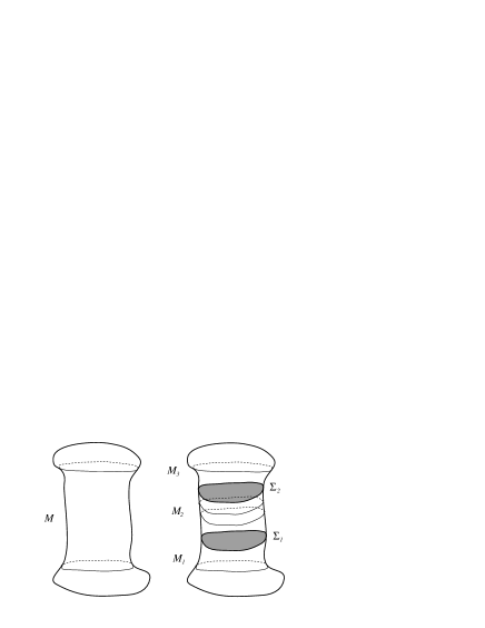
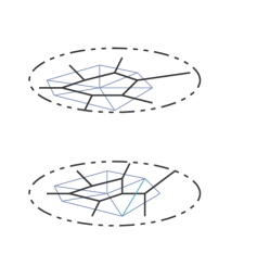
Figure 4: A possible decomposition of an orientable Manifold in three components. This drawing has only a schematic purpose since we suppose that $\partial M_{3}=-\Sigma_{2}$, $\partial M_{1}=\Sigma_{1}$ and $\partial M_{2}=\Sigma_{2}\cup-\Sigma_{1}$.

Using the previous generalization of the PRTV-model we can reinterpred the state sum model of equation (14) in the following way. As suggest by figure 4 we can imagine to split the manifold $M$ in three disjoint components glued together along the common boundary and rewrite the partition function associate to any given triangulation as:

$$TV_{G}[M^{3},\Delta] = \sum_{\vec{c}^{\prime}\in D(\gamma,G)}~{}\sum_{\vec{c}\in D(\gamma,G)}TV_{G}[{\cal S}_{2}^{\Delta_{1}^{*}};(\gamma^{\prime},c^{\prime})]\frac{1}{N(\gamma^{\prime},c^{\prime})^{2}}$$ (26)

$$\qquad TV_{G}[{\cal S}_{2}^{\Delta_{2}^{*}};(\gamma^{\prime}\cup\gamma,c+c^{\prime})]\frac{1}{N(\gamma,c)^{2}}TV_{G}[{\cal S}_{2}^{\Delta_{3}^{*}};(\gamma,c)]$$

where $\gamma\in\Sigma_{1}$ and $\gamma^{\prime}\in\Sigma_{2}$ are the graphs determined by the intersection of the 2 bone of the dual cellular decomposition $\Delta^{*}$ with $\Sigma_{1}$ and $\Sigma_{2}$, respectively. Now, getting the intersection of $\Delta^{*}$ with a 2 surface $\Sigma$ we will have that the 3 cells are mapped into 2 cells, the 2 cells are mapped into 1-cells (the edge of $\gamma$) and the 1 cells into vertices of $\gamma$. In this operation we are indeed inducing a coloring of $\gamma$ from the coloring of the branched polyhedron. Moreover, if $\Delta$ is a triangulation of $M$ then the resulting graph is trivalent. Equation (26) has a nice interpretation in terms of an operator equation. Consider the Hilbert spaces ${\cal H}_{\gamma}$ of section 2.1 associated to graphs embedded on the two Cauchy surfaces $\Sigma_{1}$ (${\cal H}_{\gamma_{1}}$) and $\Sigma_{2}$ (${\cal H}_{\gamma_{2}}$). In the normalization of [DR96] and [De 97] the completeness of ${\cal H}_{\gamma}$ is given by

$$\hat{1}_{{\gamma}}=\sum_{\vec{c}\in D(\gamma,G)}\frac{1}{N(\gamma,\vec{c})^{2}}~{}|\Sigma;\gamma,\vec{c}\rangle~{}\langle\Sigma;\gamma,{\vec{c}}|~{}~{}~{},$$ (27)

Moreover, we can define an operator $\hat{P}_{\gamma_{2},\gamma_{1}}^{(M_{2})}$

$$\hat{P}_{\gamma_{2},\gamma_{1}}^{M_{2}} : {\cal H}_{\gamma_{1}}\Longrightarrow{\cal H}_{\gamma_{2}}$$ (28)

$$\langle\gamma^{\prime},c^{\prime}|\hat{P}_{\gamma^{\prime},\gamma}^{M_{2}}|\gamma,c\rangle = TV_{G}[{\cal S}_{2}^{\Delta_{2}^{*}};(\gamma^{\prime}\cup\gamma,c+c^{\prime})].$$ (29)

This operator $\hat{P}_{\gamma^{\prime},\gamma}^{M_{2}}$ does not depends on the interior of the simple polyhedron ${\cal S}_{2}^{\Delta_{2}^{*}}$ used to compute the transition amplitude [TV92]. Using this notation we can rewrite write equation (26) as

$$TV_{G}[M^{3},\Delta]=\langle\emptyset|\hat{P}_{\emptyset,\gamma_{2}}^{M_{3}}\hat{P}_{\gamma_{2},\gamma_{1}}^{M_{2}}\hat{P}_{\gamma_{1},\emptyset}^{M_{1}}|\emptyset\rangle~{}~{}.$$ (30)

In the previous notation we have implicitly assumed that the boundary of each of the manifold $M_{i}$ can be naturally seen as made of two disjoint components ($\partial M=(\partial M)^{+}\cap(\partial M)^{-}$) one associated to the future $(\partial M)^{+}$ and the other to the past $(\partial M)^{-}$. $\hat{P}_{\gamma^{\prime},\gamma}^{M}$ is the operator of equation (29) between the Hilbert space associate to the graph $\gamma\subset-(\partial M)^{-}$ and the Hilbert space associated to the graph $\gamma^{\prime}\subset(\partial M)^{+}$. With this convention it is natural to define the composition of two manifolds with boundary $M_{1}$ and $M_{2}$ when $(\partial M)_{2}^{+}=-(\partial M)_{1}^{-}$ as the manifold $M=M_{2}\circ M1$ that one obtains gluing $M_{1}$ and $M_{2}$ along the isomorphic boundary $(\partial M)_{2}^{+}=-(\partial M)_{1}^{-}$. At this point we are ready to discus the functorial nature of the invariant. From the independence of the PRTV state sum from the chosen polyhedron we have that the $\hat{P}$ define a semifunctor on the space of manifolds with a fixed graph on their boundary:

$$\hat{P}_{\gamma^{\prime},\gamma}^{M_{2}\circ M_{1}}=\hat{P}_{\gamma^{\prime},\gamma^{\prime\prime}}^{M_{2}}\hat{P}_{\gamma^{\prime\prime},\gamma}^{M_{1}}$$ (31)

This $\hat{P}$ does not properly define a topological field theory since it is not a functor ($\hat{P}_{\gamma,\gamma}^{\Sigma\times I}\neq 1_{\gamma}$). There is however a standard procedure that allows to define a functor from a semifunctor. In fact, if we consider the Hilbert space $\overline{{\cal H}_{\gamma}}={\cal H}_{\gamma}/Ker(\hat{P}_{\gamma,\gamma}^{\Sigma\times I})$ from $\hat{P}_{\gamma^{\prime},\gamma}^{M}=\hat{P}_{\gamma^{\prime},\gamma}^{M}\circ\hat{P}_{\gamma,\gamma}^{\Sigma\times I}$ follows that its restriction to the family of Hilbert spaces $\overline{{\cal H}_{\gamma}}$ become a functor. I.e, we used the operator $\hat{P}_{\gamma,\gamma}^{\Sigma\times I}$ as the projector on the physical Hilbert space of the theory. In this way the PRTV-model defines a 2+1 dimensional quantum field theory [TV92] in the Atiyah terminology [Ati89].

From the physical point of view this discussion can be seen as a computation of Hartle-Hawking wave function and of the topology change amplitude of the 3-dimensional lattice gravity of Ponzano and Regge [Oog92a]. In consideration of a Hamiltonian (initial values) formulation in terms of loop-variable this is particularly nice. In fact, in dimension $n$ the Hamiltonian formulations is defined on an $(n-1)$ dimensional Cauchy surface and in any dimension the intersection of an $(n-1)$ surface and any 2-dimensional shadow is an 1-dimensional graph embedded on the Cauchy surface. Even more interesting is the fact the Hilbert space structure associated to the BF theory is very similar to the one of loop quantum gravity.

5 Four dimensional models

In previous section we showed how the Ponzano-Regge model correspond to the BF theory in 3 dimension. In this section we discuss an example of 4 dimensional theory that can be expressed within the spin foam formalism: the Crane-Yetter-Ooguri model of BF theory and the spin foam model of Barret and Crane. We do not discus here the model of Reisenberger [Rei97b, Rei97a]. All this models share the characteristic to be based on a theory of the BF type. This lead Freidel and Krasnov [FK98] to propose a way to systematicaly derive the spin foam model associated to any theory that admits a formulation in terms of an action of BF type plus Lagrange’s multipliers imposed constraints.

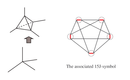
Figure 5: The elementary vertex of the BF theory. There are 5 nodes (with the associated intertwiner) and 10 links (with the associated representation). To the elementary vertex are indeed associated 15 colors.

5.1 The Crane-Yetter-Ooguri model

The state sum formulation of the topological $BF$ theory in 4-dimensions

$$Z_{BF}^{(4)} = \int[{\cal D}A(x)][{\cal D}B(x)]e^{{\rm i}\int{\rm Tr}[B\wedge F[A]]+\Lambda~{}{\rm Tr}[B\wedge B]}$$

$$= \int[{\cal D}A(x)]e^{\frac{{\rm i}}{2\Lambda}\int{\rm Tr}[F[A]\wedge F[A]]}=\int[{\cal D}A(x)]e^{\frac{{\rm i}}{2\Lambda}\int d\big{(}{\rm Tr}[A\wedge F[A]]+\frac{2}{3}{\rm Tr}[A\wedge A\wedge A]\big{)}}$$

with cosmological constant is given by the Crane-Yetter [CKY97] or by the Ooguri (without cosmological constant) [Oog92b] models. The partition function of the model associated to a triangulation $\Delta$ of a manifold $M$ can be written as :

$$Z_{BF}(\Delta,\Lambda)=\sum_{j_{f},i_{t}}\prod_{f}dim_{q}(j_{f})\prod_{v}\phi_{q,v}(\vec{\jmath},\vec{\imath}),$$ (33)

where $q=\exp({\rm i}\Lambda)$, $j_{f}$ denotes a coloring of the faces of $\Delta$ by irreducible representation of $U_{q}(su(2))$, $i_{t}$ denotes a coloring of the tetrahedra of $\Delta$ by intertwiners and the sum is over all such colorings with $j<{\pi\over\Lambda}$. Moreover $dim_{q}(j)$ denotes the quantum dimension of the representation of spin $j$ and $\phi_{v}(\vec{\jmath},\vec{\imath})$ denote the quantum $15$-j symbol associated with the 4-simplex $v$. More precisely, associated to a 4-simplex $v$ we consider a graph $\Gamma_{v}$ given by the intersection between the 2-skeleton of the complex which is dual to the triangulation and the boundary of the 4-simplex $v$ (see figure 5). $\Gamma_{v}$ corresponds to the pentagram graph and we color its 10 edges by $\vec{j}$ and its 5 vertices by $\vec{i}$. $\phi_{q,v}(\vec{\jmath},\vec{\imath})$ corresponds to the Reshetikhin-Turaev evaluation of the colored graph $\Gamma_{v}$. This state sum does not depend on the triangulation when correctly normalized by a factor $N^{n_{0}-n_{1}}$, where $n_{0},n_{1}$ is the number of $0,1$ simplices, and it corresponds to the evaluation of the BF partition function of equation (5.1).

5.2 The Barret-Crane model

The Relativistic-Spin-Foam model is a modification of the state sum (5.1) in the case of the $so(4)$ gauge group in which the conditions corresponding to the quantum 4-simplex conditions (when $\Lambda=0$) are imposed by hand. Yetter generalized this construction to the case of non vanishing $\Lambda$ [Yet98]. Yetter emphasized that the quantum group that should be considered is $U_{q}(su(2))\otimes U_{q^{-1}}(su(2))$. This state sum model can be written :

$$Z_{BC}(\Delta,\Lambda) = \sum_{j_{f},\jmath^{\prime}_{f},i_{t},\imath^{\prime}_{t}}\prod_{f}dim_{q}(j_{f})dim_{q^{-1}}(\jmath^{\prime}_{f})\prod_{v}\phi_{q,v}(\vec{\jmath},\vec{\imath})\phi_{q^{-1},v}(\vec{\jmath^{\prime}},{\vec{\imath^{\prime}}})\delta_{\vec{\jmath},\vec{\jmath^{\prime}}}\delta_{\vec{\imath},\vec{\imath^{\prime}}}.$$ (34)

So this model corresponds to two copies of $su(2)$ $BF$ theories (or an $so(4)$ $BF$ theory) together with $15$ constraints imposed for each 4-simplex. The presence of $\delta_{\vec{j},\vec{\jmath^{\prime}}}$ and $\delta_{\vec{i},\vec{\imath^{\prime}}}$ corresponds to the geometricity constraint. In [DF98] it is shown that the above spin foam model can be associated to a well defined field action: the $so(4)$ Plebanski action [Ple77]. This is a deformed BF theory depending on an $so(4)$ connection $\omega=\omega_{\mu}^{IJ}X_{IJ}dx^{\mu}$, a two form valued into $so(4)$ $B=B^{IJ}_{\mu\nu}X_{IJ}dx^{\mu}\wedge dx^{\nu}$, and a scalar symmetric traceless matrix $\phi_{[IJ][KL]}$ ($\epsilon^{IJKL}\phi_{IJKL}=0$) that acts as Lagrange multiplier fields. This action reads:

$${\cal S}[\omega;B;\phi] = \int_{M}\!\!\!\bigg{[}B^{IJ}\wedge F_{IJ}(\omega)-\frac{\Lambda}{4}\epsilon_{IJKL}B^{IJ}\wedge B^{KL}-\frac{1}{2}\phi(B)_{IJ}\wedge B^{IJ}\bigg{]}~{},$$ (35)

where $\phi(B)_{IJ}=\phi_{IJKL}B^{KL}$. In this context, the geometry constraints are imposed, at the quantum level, by the integration over Lagrange multiplier fields $\phi_{[IJ][KL]}$. This action has two nice characteristics: (1) one of its sectors of solution is closely connected to gravity; (2) it is a deformation of a quantizable topological theory (The BF theory) that can play a role analogous to the one of free theory in standard quantum field theory. Moreover, it is intriguing that this description of gravity as a constraint BF theory can be generalized to higher dimension [FKP99].

6 Conclusion

In this work we showed that the spin foam formalism gives an unified framework for the discussion of an important class of diff-invariant quantum theories. Between them: topological BF theory in 3 and 4 dimension, the four dimensional formulation of loop quantization of gravity, the Barret-Crane model. The main unsolved problems of the general picture we described here are:

1. The state sum model we described are properly defined only on a single given triangulation (or its dual spin-foam). If this is fine in the case of a topological field theory without local degree of freedom this is questionable in the case of gravity. Work is now in progress [DR] on the direction of dealing with all the possible triangulation. This is somehow analogue to consider generalization (where the triangulation is not the only dynamical variable) of the model of dynamical triangulations [ACM97].

2. The connection between the spin foam models and the exponential of the constraints need to be improved with a rigorous mathematical analysis of the derivation.

3. A systematical study of the physical implication of taking different weight factor is missing.

Acknowledgment:
This work was greatly influenced by numerous discussion with M. Carfora, L. Freidel, J. Lewandowski, L. Lusanna, A. Marzuoli, M. Pauri, C. Rovelli and J. Zapata, to whom all I’m extremely grateful. The work of R.D.P. at CPT Marseille is supported by a Dalla Riccia Fellowship.

References

- [ABCK98] A. Ashtekar, J. Baez, A. Corichi, and K. Krasnov, Quantum geometry and black hole entropy, Phys. Rev. Lett. 80 (1998), 904–907.
- [ACM97] Jan Ambjorn, Mauro Carfora, and Annalisa Marzuoli, The geometry of dynamical triangulations, Lecture Notes in Physics, vol. LNP m50, Springer-Verlag, Berlin, 1997.
- [AI92] Abhay Ashtekar and C. J. Isham, Inequivalent observable algebras: Another ambiguity in field quantization, Phys. Lett. B274 (1992), 393–398.
- [AL95] Abhay Ashtekar and Jerzy Lewandowski, Differential geometry on the space of connections via graphs and projective limits, J. Geom. Phys. 17 (1995), 191.
- [AL97] Abhay Ashtekar and Jerzy Lewandowski, Quantum theory of geometry. 1: Area operators, Class. Quant. Grav. 14 (1997), A55–A82.
- [AL98] Abhay Ashtekar and Jerzy Lewandowski, Quantum theory of geometry. 2. volume operators, Adv. Theor. Math. Phys. 1 (1998), 388.
- [ALM+95] Abhay Ashtekar, Jerzy Lewandowski, Donald Marolf, Jose Mourao, and Thomas Thiemann, Quantization of diffeomorphism invariant theories of connections with local degrees of freedom, J. Math. Phys. 36 (1995), 6456–6493.
- [Ash86] A. Ashtekar, New variables for classical and quantum gravity, Phys. Rev. Lett. 57 (1986), 2244.
- [Ati89] M. Atiyah, Topological quantum field theories, Publ. Math. IHES 68 (1989), 175–186.
- [AW91] Francis Archer and Ruth M. Williams, The turaev-viro state sum model and three-dimensional quantum gravity, Phys. Lett. B273 (1991), 438–444.
- [Bae94] John C. Baez, Generalized measures in gauge theory, Lett. Math. Phys. 31 (1994), 213–224.
- [Bae98] John C. Baez, Spin foam models, Class. Quant. Grav. 15 (1998), 1827.
- [Bar95] J. Fernando Barbero, Real ashtekar variables for lorentzian signature space times, Phys. Rev. D51 (1995), 5507–5510.
- [Bar96] J. Fernando Barbero, From euclidean to lorentzian general relativity: The real way, Phys. Rev. D54 (1996), 1492–1499.
- [BC98] John W. Barrett and Louis Crane, Relativistic spin networks and quantum gravity, J. Math. Phys. 39 (1998), 3296–3302.
- [BCR96] Marcelo Barreira, Mauro Carfora, and Carlo Rovelli, Physics with nonperturbative quantum gravity: Radiation from a quantum black hole, Gen. Rel. Grav. 28 (1996), 1293.
- [BDR97] Roumen Borissov, Roberto De Pietri, and Carlo Rovelli, Matrix elements of thiemann’s hamiltonian constraint in loop quantum gravity, Class. Quant. Grav. 14 (1997), 2793.
- [CCM98] Gaspare Carbone, Mauro Carfora and Annalisa Marzuoli Wigner symbols and combinatorial invariants of 3-manifolds with boundary, SISSA preprint 118/98/FM.
- [CKS98] J. Scott Carter, Louis H. Kauffman, and Masahico Saito, Structures and diagrammatics of four-dimensional topological lattice field theories, xxx-archive:math.GT/9806023.
- [CKY97] Louis Crane, Louis H. Kauffman, and David N. Yetter, State sum invariants of four manifolds., J. Knot Theory Ramifications 6 (1997), no. 2, 177–234, xxx-archive:hep-th/9409167.
- [De 97] Roberto De Pietri, On the relation between the connection and the loop representation of quantum gravity, Class. Quant. Grav. 14 (1997), 53–70.
- [DF98] R. De Pietri and L. Freidel, so(4) plebanski action and relativistic spin foam model, xxx-archive:gr-qc/980471.
- [DR] Roberto De Pietri and Carlo Rovelli, In preparation.
- [DR96] Roberto De Pietri and Carlo Rovelli, Geometry eigenvalues and scalar product from recoupling theory in loop quantum gravity, Phys. Rev. D54 (1996), 2664–2690.
- [FK98] Laurent Freidel and Kirill Krasnov, Spin foam models and the classical action principle, Adv. Theor. Math. Phys. 2 (1998), 1221-1285.
- [FKP99] Laurent Freidel, Kirill Krasnov and Raimond Puzio, BF Description of Higher-Dimensional Gravity Theories, xxx-archive:hep-th/9901069.
- [Hor89] Gary T. Horowitz, Exactly soluble diffeomorphism invariant theories, Comm. Math. Phys. 125 (1989), 417.
- [KL94] Louis H. Kauffman and S. L. Lins, Temperley-lieb recoupling theory and invariant of 3-manifolds, Princeton University Press, Princeton, 1994.
- [Kra97] Kirill V. Krasnov, Geometrical entropy from loop quantum gravity, Phys. Rev. D55 (1997), 3505–3513.
- [Oog92a] Hirosi Ooguri, Partition functions and topology changing amplitudes in the 3-d lattice gravity of ponzano and regge, Nucl. Phys. B382 (1992), 276–304.
- [Oog92b] Hirosi Ooguri, Topological lattice models in four-dimensions, Mod. Phys. Lett. A7 (1992), 2799–2810.
- [OS91] Hirosi Ooguri and Naoki Sasakura, Discrete and continuum approaches to three-dimensional quantum gravity, Mod. Phys. Lett. A6 (1991), 3591–3600.
- [Pen71] Roger Penrose, Application of negative dimension tensor, Combinatorial mathematics and its applications (D. J. Welsh, ed.), Academic Press, New Jork, 1971, pp. 221–243.
- [Ple77] J. Plebanski, On the separations of eisteinian substructure, J. Math. Phys. 18 (1977), 2511.
- [PR68] G. Ponzano and T Regge, Semiclassical limit of racach coefficients, Spetroscopy and group theoretical methods in Physics (F. Bloch, ed.), North-Holland, Amsterdam, 1968.
- [Rei94] Michael P. Reisenberger, World sheet formulations of gauge theories and gravity, xxx-archive:gr-qc/9412035.
- [Rei95] Michael P. Reisenberger, New constraints for canonical general relativity, Nucl. Phys. B457 (1995), 643–687.
- [Rei97a] Michael P. Reisenberger, A lattice world sheet sum for 4-d euclidean general relativity, xxx-archive:gr-qc/9711052.
- [Rei97b] Michael P. Reisenberger, A lefthanded simplicial action for euclidean general relativity, Class. Quant. Grav. 14 (1997), 1753.
- [Rei98] Michael P. Reisenberger, Classical euclidean general relativity from ’lefthanded area = righthanded area’, xxx-archive:gr-qc/9804061.
- [Rov96] Carlo Rovelli, Black hole entropy from loop quantum gravity, Phys. Rev. Lett. 77 (1996), 3288.
- [Rov98a] Carlo Rovelli, Loop quantum gravity, Living Reviews in Relativity, no. 1998-1, Max-Planck-Institut für Gravitationsphysik (Albert-Einstein-Institut), 1998, http://www.livingreviews.org.
- [Rov98b] Carlo Rovelli, The projector on physical states in loop quantum gravity, xxx-archive:gr-qc/9806121.
- [Rov98c] Carlo Rovelli, Strings, loops and others: A critical survey of the present approaches to quantum gravity, Gravitation and Relativity: At the turn of the Millennium (Pune, India) (N. Dadhich and J. Narlikar, eds.), Proceeding of the GR15 Conference, I.U.C.A.A., December, 16 -21 1998, p. 281.
- [RR97] Michael P Reisenberger and Carlo Rovelli, ’sum over surfaces’ form of loop quantum gravity, Phys. Rev. D56 (1997), 3490–3508.
- [RS72] C. P. Rourke and B. J. Sanderson, Introduction to picewise-linear topology, Springer-Verlag, Berlin, 1972.
- [RS88] Carlo Rovelli and Lee Smolin, Knot theory and quantum gravity, Phys. Rev. Lett. 61 (1988), 1155.
- [RS90] Carlo Rovelli and Lee Smolin, Loop space representation of quantum general relativity, Nucl. Phys. B331 (1990), 80.
- [RS95a] Carlo Rovelli and Lee Smolin, Discreteness of area and volume in quantum gravity, Nucl. Phys. B442 (1995), 593–622, erratum: Nucl. Phys. B442,(1995),xxx.
- [RS95b] Carlo Rovelli and Lee Smolin, Spin networks and quantum gravity, Phys. Rev. D52 (1995), 5743–5759.
- [Thi96] T. Thiemann, Anomaly - free formulation of nonperturbative, four- dimensional lorentzian quantum gravity, Phys. Lett. B380 (1996), 257–264.
- [Thi98a] T. Thiemann, Quantum spin dynamics (qsd), Class. Quant. Grav. 15 (1998), 839.
- [Thi98b] T. Thiemann, Quantum spin dynamics (qsd). 2, Class. Quant. Grav. 15 (1998), 875.
- [Thi98c] T. Thiemann, Qsd 3: Quantum constraint algebra and physical scalar product in quantum general relativity, Class. Quant. Grav. 15 (1998), 1207.
- [TV92] V. G. Turaev and O. Y. Viro, State sum invariant of 3-manifolds and quantum 6j-symbols, Topology 31 (1992), no. 4, 865–902.
- [Wit88a] Edward Witten, (2+1)-dimensional gravity as an exactly soluble system, Nucl. Phys. B311 (1988), 46.
- [Wit88b] Edward Witten, Topological gravity, Phys. Lett. 206B (1988), 601.
- [Wit88c] Edward Witten, Topological quantum field theory, Commun. Math. Phys. 117 (1988), 353.
- [Wit89a] Edward Witten, Quantum field theory and the jones polynomial, Commun. Math. Phys. 121 (1989), 351.
- [Wit89b] Edward Witten, Topology changing amplitudes in (2+1)-dimensional gravity, Nucl. Phys. B323 (1989), 113.
- [Yet98] David N. Yetter, Generalised barrett-crane vertices and invariants of embedded graphs, xxx-archive:math.QA/9801131.
- [Zap97] Jose A. Zapata, A combinatorial approach to diffeomorphism invariant quantum gauge theories, J. Math. Phys. 38 (1997), 5663–5681.
- [Zap98] Jose A. Zapata, Combinatorial space from loop quantum gravity, Gen. Rel. Grav. 30 (1998), 1229.