Timing Effects of Gravitational Waves from Localized Sources

Localized astronomical sources like a double stellar system, rotating neutron star, or a massive black hole at the center of the Milky Way emit periodic gravitational waves. For a long time only a far-zone contribution of gravitational fields of the localized sources (plane-wave-front approximation) were a matter of theoretical analysis. We demonstrate how this analysis can be extended to take into account near-zone and intermediate-zone contributions as well. The formalism is used to calculate gravitational-wave corrections to the Shapiro time delay in binary pulsars and low-frequency (LF) pulsar timing noise produced by an ensemble of double stars in our galaxy.

1 Introduction

The extremely high precision of current pulsar timing observations demands a better theoretical treatment of secondary effects in the propagation of electromagnetic signals in variable gravitational fields of oscillating and precessing stars, or binary systems. Especially important is the problem of propagation of light rays in the field of gravitational waves emitted by a localized source of gravitational radiation. A consistent approach for a complete and exhaustive solution of this problem has been developed in papers $\!{}^{{\bf?}}$^-$\!{}^{{\bf?}}$ in the first post-Minkowskian approximation of General Relativity. We have demonstrated for the first time that the equations of light propagation in the retarded gravitational field of an arbitrary localized source emitting gravitational waves can be integrated exactly in closed form. It allows to examine the influence of the time-dependent gravitational field on the light propagation not only in the wave zone but also in cases when light passes through the intermediate and near zones of the source. We have obtained explicit analytic expressions for light deflection and integrated time delay (Shapiro effect) accounting for all possible retardation effects and arbitrary relative locations of the source of gravitational waves, the source of light rays , and the observer. Coordinate dependent terms in the expressions for observable quantities were singled out and used for the unique interpretation of observable effects. Our exploration essentially extends previous results regarding propagation of light rays in the field of a plane monochromatic gravitational wave (see, e.g., papers $\!{}^{{\bf?}}$^-$\!{}^{{\bf?}}$) and significantly surpasses theoretical approaches of other authors $\!{}^{{\bf?}}$^-$\!{}^{{\bf?}}$. In the present paper we briefly discuss the developed formalism and apply it to describe the Shapiro time delay in binary pulsars as well as to estimate the intensity of LF timing noise produced by an ensemble of double stars of our galaxy.

2 Propagation of light in time-dependent gravitational fields

We solve the Einstein equations in the first post-Minkowskian approximation where the metric tensor $g_{\alpha\beta}$ is decomposed linearly into the Minkowski metric $\eta_{\alpha\beta}$ and a small perturbation $h_{\alpha\beta}$,

$$g_{\alpha\beta}=\eta_{\alpha\beta}+h_{\alpha\beta}\;.$$ (1)

The Einstein equations for $h_{\alpha\beta}$ in harmonic gauge read

$$\mathop{\kern 1.0pt\hbox{${\vbox{\hrule height=0.4pt\hbox{\vrule width=0.4pt,height=8.0pt\kern 8.0pt\vrule width=0.4pt} \hrule height=0.4pt}}$}\kern 1.0pt}h_{\alpha\beta}(t,{\bf x})=-16\pi S_{\alpha\beta}(t,{\bf x})\;,\quad\quad\mbox{where}\quad\quad S_{\alpha\beta}(t,{\bf x})=T_{\alpha\beta}(t,{\bf x})-\frac{1}{2}\eta_{\alpha\beta}\;T_{\;\;\lambda}^{\lambda}(t,{\bf x})\;.$$ (2)

Herein $T^{\alpha\beta}$ is the tensor of energy-momentum of a system of massive particles $\!{}^{{\bf?}}$

$$T^{\alpha\beta}(t,{\bf x})=\sum_{a=1}^{N}\hat{T}_{a}^{\alpha\beta}(t)\delta\left({\bf x}-{\bf x}_{a}(t)\right)\;,\quad\quad\quad\quad\quad\hat{T}_{a}^{\alpha\beta}(t)=m_{a}\gamma_{a}^{-1}(t)u_{a}^{\alpha}(t)u_{a}^{\beta}(t)\;,$$ (3)

where $t$ is coordinate time, ${\bf x}=x^{i}=(x^{1},x^{2},x^{3})$ denotes spatial coordinates of a current point in space, $m_{a}$ and ${\bf x}_{a}(t)$ are the rest mass and spatial coordinates of the $a$-th particle, ${\bf v}_{a}(t)=d{\bf x}_{a}(t)/dt$, $\gamma_{a}(t)=[1-v_{a}^{2}(t)]^{-1/2}$ is the Lorentz factor, $u_{a}^{\alpha}(t)=\{\gamma_{a}(t),\;\gamma_{a}(t){\bf v}_{a}(t)\}$ is the four-velocity of the $a$-th particle, $\delta({\bf x})$ is the 3-dimensional Dirac delta-function. The solution of (2) is the retarded Liénard-Wiechert tensor potential

$$h^{\alpha\beta}(t,{\bf x}) = 4\sum_{a=1}^{N}\;\frac{\hat{T}_{a}^{\alpha\beta}(s)-\frac{1}{2}\eta^{\alpha\beta}\hat{T}_{a\lambda}^{\lambda}(s)}{r_{a}(s)-{\bf v}_{a}(s)\cdot{\bf r}_{a}(s)}\;,$$ (4)

where the retarded time $s=s(t,{\bf x})$ for the $a$-th body is a solution of the light-cone equation $s+|{\bf x}-{\bf x}_{a}(s)|=t$. Here it is assumed that the field is measured at time $t$ and at the point ${\bf x}$.

We consider the motion of a light ray (photon) in the background gravitational field described by the metric (4). The motion of the photon is defined by solving equations of a light geodesic (see Fig 1). The original equations of propagation of light rays are rather complicated $\!{}^{{\bf?}}$. They can be simplified and reduced to a form which allows to resort to a special approximation method for their integration. The reduced equations and details of the integration procedure can be found in our paper $\!{}^{{\bf?}}$. In what follows we discuss some of physical applications of the mathematical technique.

Figure 1: Illustration of the light-ray’s propagation history. The light ray is emitted at the instant of time $t_{0}$ at the point ${\bf x}_{0}$ and arrives at the point of observation ${\bf x}$ at the instant of time $t$. Light-deflecting bodies moves along accelerated world lines during the time of propagation of the light ray; their velocities at some intermediate instant of time are shown by black arrows. In the absence of the light-ray-deflecting bodies the light ray would propagate along an unperturbed path (dashed line) which is a straight line passing through the points of emission, ${\bf x}_{0}$, and observation, ${\bf x}$. Direction of the unperturbed path is determined by the unit vector ${\bf K}=-({\bf x}-{\bf x}_{0})/|{\bf x}-{\bf x}_{0}|$. In the presence of the light-ray-deflecting bodies the light ray propagates along the perturbed path (solid line). The perturbed trajectory of the light ray is bent and twisted due to the gravito-electric (mass-induced) and gravito-magnetic (velocity-induced) fields of the bodies. The initial boundary condition for the equation of light propagation is determined by the unit vector ${\bf k}$ defined at past null infinity by means of a dynamical backward-in-time prolongation (dotted line) of the perturbed trajectory of light from the point of emission ${\bf x}_{0}$ in such a way that the tangent vector of the prolongated trajectory coincides with that of the perturbed light-ray’s trajectory at the point of emission. The relationship between unit vectors ${\bf k}$ and ${\bf K}$ includes relativistic bending of light.

3 Shapiro time delay in binary pulsars

Damour & Esposito-Farèse $\!{}^{{\bf?}}$ argued about the contribution of gravitational waves emitted by a binary pulsar to the observed Shapiro time delay. As a consequence of the main result of their work they claimed that the contribution probably should be small. However, they were not able to present conclusive mathematical arguments which are given in this section.

The general formalism of our paper $\!{}^{{\bf?}}$ yields for the time of propagation of the light-ray

$$t-t_{0} = |{\bf x}-{\bf x}_{0}|+\Delta(t,t_{0})\;,$$ (5)

where $|{\bf x}-{\bf x}_{0}|$ is the Euclidean distance between the points of emission, ${\bf x}_{0}$, and observation, ${\bf x}$, of the photon, and $\Delta(t,t_{0})$ is the Shapiro time delay due to the gravitational field of moving bodies

$$\Delta(t,t_{0}) = \frac{1}{2}k_{\alpha}k_{\beta}B^{\alpha\beta}(\tau)-\frac{1}{2}k_{\alpha}k_{\beta}B^{\alpha\beta}(\tau_{0})\;=\;2\sum_{a=1}^{2}m_{a}\;B_{a}(s,s_{0})\;,$$ (6)

$$B_{a}(s,s_{0}) = \displaystyle{\int^{s}_{s_{0}}}\frac{[1-{\bf k}\cdot{\bf v}_{a}(\zeta)]^{2}}{\sqrt{1-v^{2}_{a}(\zeta)}}\frac{d\zeta}{t^{\ast}+{\bf k}\cdot{\bf x}_{a}(\zeta)-\zeta}\;,$$ (7)

where the retarded time $s$ is obtained by solving the equation of light cone for the time of observation, the time $s_{0}$ is found by solving the same equation written down for the time of emission of photon $s_{0}+|{\bf x}_{0}-{\bf x}_{a}(s_{0})|=t_{0}$, and $t^{\ast}$ is the (constant) time of the closest approach of the light ray to the origin of the coordinate system used for calculations. Choosing the origin of the coordinate system to be the barycenter of the binary pulsar, expanding (7) in powers of $v_{a}/c$, and performing integration result in $\!{}^{{\bf?}}$

$$\Delta(t,t_{0}) = -2m_{c}(1-{\bf k}\cdot{\bf v}_{c})\ln\left[\left(r+{\bf k}\cdot{\bf r}\right)-{\bf v}_{c}\cdot{\bf r}+({\bf k}\cdot{\bf r})({\bf k}\cdot{\bf v}_{c})\right]\;,$$ (8)

where $m_{c}$ is the mass of the pulsar’s companion, ${\bf r}$ is the radial distance between the pulsar and companion, ${\bf v}_{c}$ is the companion’s barycentric velocity, and all quantities are taken at the barycentric time of emission of the pulsar’s radio pulse. Formula (8) apparently demonstrates that the velocity-dependent terms present in the Shapiro effect are small and only marginally detectable in timing of binary pulsars. This proves the intuitive guess of the paper $\!{}^{{\bf?}}$. Formula (8) can be implemented in the parameterized post-Keplerian formalism $\!{}^{{\bf?}}$^,$\!{}^{{\bf?}}$. Its explicit formulation is given in $\!{}^{{\bf?}}$. In case of circular orbits it reads

$$\Delta_{S} = -\frac{2Gm_{c}}{c^{3}}\ln\biggl{\{}1-\sin i\left[\sin\left(\varphi-\varphi_{0}\right)+\frac{x}{P_{b}}\frac{m_{p}}{m_{c}}\;\pi\sin 2\left(\varphi-\varphi_{0}\right)\right]\biggr{\}}\;,$$ (9)

where $m_{p}$ is the pulsar’s mass, $\varphi$ is the orbital phase, $\varphi_{0}$ is constant, $x$ is the projected semi-major axis of the orbit, $P_{b}$ is the orbital period, and we have restored $G$ and the speed of light $c$ for convenience. The correction to the Shapiro delay given in (9) may be observed in binary pulsars with orbits visible nearly edgewise.

4 Low-frequency pulsar timing noise

Each double star in our galaxy emits rather weak LF gravitational waves. However, an ensemble of double stars may produce a noticeable amount of the gravitational radiation which could be detected through the analysis of the long-term behavior of the timing residuals (see Fig. 2). Time variations caused by quadrupolar gravitational waves from a double star read as $\!{}^{{\bf?}}$

$$\Delta(t,t_{0}) = \delta(t,r,\theta)-\delta(t_{0},r_{0},\theta_{0})\;,$$ (10)

$$\delta(t,\theta,r)=\frac{k^{i}k^{j}}{1-\cos\theta}\left[\frac{\dot{\cal I}_{ij}^{TT}(t-r)}{r}+\frac{1}{1-\cos\theta}\;\frac{{\cal I}_{ij}^{TT}(t-r)}{r^{2}}+\frac{A(\theta,t-r)}{r^{2}}\right]+O\left(r^{-3}\right)\;,$$ (11)

where $k^{i}$ is the unit vector from the pulsar towards the observer, $r$ is the distance ‘observer-double star’; $r_{0}$ is the distance ‘pulsar-double star’ ($r_{0}=(r^{2}+R^{2}-2rR\cos\theta)^{1/2}$); $\theta$ is the angle between the directions ‘observer-double star’ and ‘observer-pulsar’; $\theta_{0}$ is the angle between the directions ‘pulsar-double star’ and ‘observer-pulsar’; ${\cal I}_{ij}^{TT}$ is the transverse-traceless quadrupole moment of the double star; $A(\theta,t-r)$ is a regular function. If one takes a particular event of a circular orbit the formula (11) is brought to the form

$$\delta(t,\theta,r) = \frac{(G{\cal M})^{5/3}}{c^{4}\;\omega^{1/3}}\frac{\cos^{2}\displaystyle{\frac{\theta}{2}}}{r}\left[(1+\cos^{2}i)\cos 2\Omega\sin 2\varphi+2\cos i\sin 2\Omega\cos 2\varphi\right]$$

$$-\frac{(G{\cal M})^{5/3}}{4c^{3}\;\omega^{4/3}}\frac{\cot^{2}\displaystyle{\frac{\theta}{2}}}{r^{2}}\left[(1+\cos^{2}i)\cos 2\Omega\cos 2\varphi-2\cos i\sin 2\Omega\sin 2\varphi\right]+O\left(\frac{G^{5/3}{\cal M}^{5/3}}{c^{2}\omega^{7/3}r^{3}}\right)\;,$$

where $\varphi=\omega t+\sigma$ is the orbital phase of the double star, $\sigma$ is constant, $\omega=2\pi\nu$ is the orbital frequency, $\Omega$ is the longitude of the ascending node, and ${\cal M}=(m_{1}m_{2})^{3/5}(m_{1}+m_{2})^{-1/5}$ is the ”chirp” mass of the double star.

An ensemble of double stars generates the gravitational wave noise with the autocovariance function ${\cal R}(\tau)$ defined as the ensemble average of products of the time delay (10)

$${\cal R}(\tau) = <\Delta(t,t-R)\;\Delta(t+\tau,t-R+\tau)>\;,$$ (13)

where we have used an approximation $t_{0}=t-R$. The ensemble averaging is defined with respect to the set of random variables $\Omega$, $i$, $\varphi_{0}$, $\nu$, $\theta$, and $r$ . We assume that the variables $\Omega$, $i$, $\varphi_{0}$ are distributed uniformly. The probability distribution function of other variables of the ensemble is determined by main-sequence galactic double stars which occupy the frequency band $\!{}^{{\bf?}}$ from $10^{-13}$ to $10^{-5}$ Hz with the frequency and spatial distributions $F(\nu)$ and $n({\bf r})$ respectively

$$\frac{dN(\nu,{\bf r})}{d\nu\;d{\bf r}}=F(\nu)n({\bf r})\;,\quad\quad\quad\quad F(\nu)=\frac{\kappa(\nu)}{\nu}\;,$$ (14)

where it has been assumed that $F(\nu)$ and $n({\bf r})$ are statistically independent. Function $\kappa(\nu)$ is almost constant over a wide range of frequencies. Hence, we take $F(\nu)\simeq 0.054/\nu$.

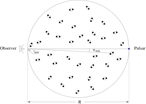
Figure 2: A model of an ensemble of double systems producing LF gravitational noise. The minimal distance observer-double star is denoted as $r_{min}$ and the minimal angle between directions to the pulsar and a double star is denoted as $\theta_{min}$. The distance from the observer to the pulsar is $R$. Concentration, $n$, of double stars is assumed to be constant. Then, $r_{min}\sim n^{-1/3}$, $\theta_{min}\sim r_{min}/R$, and $n({\bf r})=3n/(4\pi R^{3})$.

One can prove that the double-star-gravitational-wave noise is stationary with spectrum $S(\nu)$ defined by the Fourier transform of the autocovariance function. The spectrum has the following specific properties

• the noise consists of seven components having spectra $S(\nu)\sim\nu^{-5/3-\alpha}$ ($\alpha=0\div 6$);

• the amplitude of any component of the noise crucially depends on the spatial distribution of galactic double stars between the observer and the pulsar as well as in the neighborhood of each (e.g. a pulsar in a globular cluster);

• the component of $S(\nu)$ with $\alpha=0$ is produced by the far zone gravitational field ($\sim r^{-1}$) of double stars (pure gravitational waves) and is regular everywhere including the line of sight of observer towards the pulsar, when $\theta=0$;

• the component of $S(\nu)$ with $\alpha=2$ is due to the semi-far zone gravitational field ($\sim r^{-2}$) of double stars and diverges along the line of sight of observer towards the pulsar ;

• the components of $S(\nu)$ with $\alpha=4,6$ are due to the intermediate zone ($\sim r^{-3}$) and near zone ($\sim r^{-4}$) gravitational fields of double stars and are regular everywhere.

In order to give an estimate of the expected amount of the gravitational wave noise in pulsar timing we use a simple model of uniform distribution of double stars in the spherical domain between the pulsar and observer at the Earth (see Fig. 2 for more details). The strength of the timing noise is most conveniently characterized by the, so-called, $\sigma_{z}$ statistic $\!{}^{{\bf?}}$ defined as

$$\sigma_{z}(\tau) = \frac{\tau^{2}}{2\sqrt{5}}<c_{3}^{2}(\tau)>^{1/2}\;,$$ (15)

where $c_{3}(\tau)$ is a random variable being proportional to the statistical fluctuations of the third time derivative of the pulsar’s timing residuals, $r(t)$, and $\tau$ is the total span of observational time. In the case of a single double star, ${\em r}(t)=\Delta(t,t-R)$. In what follows we simplify the problem by accounting for only the line-of-sight divergent component of $\Delta(t,t-R)$ given in the second line of (4). Performing integration over the ensemble’s variables and over the sperical volume shown in Fig. 2 gives

$$<c_{3}^{2}(\tau)>\simeq(2\pi)^{6}\int_{0}^{1/\tau}\nu^{6}S(\nu)d\nu\;,\quad\quad\mbox{with}\quad\quad S(\nu)\sim\nu^{-11/3}\;,\quad\quad\mbox{so that}$$ (16)

$$\sigma_{z}(\tau) \simeq 0.7\cdot 10^{-18}\left(\frac{\cal M}{{\cal M}_{\odot}}\right)^{5/3}\left(\frac{n}{{\rm 1}\;{\rm pc}^{3}}\right)\left(\frac{R}{\mbox{1 kpc}}\right)\left(\frac{\tau}{\mbox{1 yr}}\right)^{1/3}\;.$$ (17)

This limit is lower than that presently accessible in the timing of millisecond pulsars. However, we emphasize that the estimate (17): 1) is model dependent, and 2) contribution of several other components of $\Delta(t,t-R)$ were neglected. It is highly desirable to repeat our calculations with more realistic ensemble of double star distributions and the complete account for all constituents of $\Delta(t,t-R)$. We argue that proceeding in this way the origin of the incomprehensible ‘red’ timing noise discovered in PSR B1937+21 $\!{}^{{\bf?}}$ may be explained as a result of the LF gravitational wave noise from double stars in our galaxy - a challenge both for theorists and observers.

References

References

• [1] Kopeikin, S.M., J. Math. Phys. 38, 2587 (1997)
• [2] Kopeikin, S.M., SchΓ€fer G., Gwinn, C.R., & Eubanks, T.M., Phys. Rev. D, in press, e-print astro-ph/9811003
• [3] Kopeikin, S.M. & SchΓ€fer, G., submitted to Phys. Rev. D, e-print gr-qc/9902030
• [4] Mashhoon, B. & Seitz, M., Mon. Not. R. Astron. Soc. 249, 84 (1991)
• [5] Durrer, R., Phys. Rev. Lett. 72, 3301 (1994)
• [6] Pyne, T., Gwinn, C.R., Birkinshaw, M., Eubanks, T.M. & Matsakis, D.N., Astrophys. J. 465, 566 (1996)
• [7] Kaiser, N. & Jaffe, A., Astrophys. J. 484, 545 (1997)
• [8] Plebanski, J., Phys. Rev. 118, 1396 (1960)
• [9] Stebbins, A., Astrophys. J. 327, 584 (1988)
• [10] Kovner, I., Astrophys. J. 351, 114 (1990)
• [11] Pyne, T. & Birkinshaw, M., Astrophys. J. 415, 459 (1993)
• [12] Damour, T., & Esposito-FarΓ¨se, G., Phys. Rev. D 58, 044003 (1998)
• [13] Landau, L.D. & Lifshitz, E.M., 1971, The Classical Theory of Fields, Pergamon: Oxford
• [14] Damour, T. & Deruelle, N., Ann. Inst. H. PoincarΓ© A44, 263 (1986)
• [15] Damour, T. & Taylor, J.H., Phys. Rev. D 45, 1840 ( 1992)
• [16] Allen, C., Poveda, A. & Herrera, M.A., In: Visual Double Stars: Formation, Dynamics and Evolutionary Tracks, eds. J.A. Docobo, A. Elipe & McAlister, H., Kluwer: Dordrecht (1997), pp. 133-143
• [17] Taylor, J.H., IEEE 79, 1054 (1991)
• [18] Kaspi, V.M., Taylor, J.H. & Ryba, M.F., Astrophys. J. 428, 713 (1994)