The Generalized Hartle-Hawking Initial State: Quantum Field Theory on Einstein Conifolds

Abstract

Recent arguments have indicated that the sum over histories formulation of quantum amplitudes for gravity should include sums over conifolds, a set of histories with more general topology than that of manifolds. This paper addresses the consequences of conifold histories in gravitational functional integrals that also include scalar fields. This study will be carried out explicitly for the generalized Hartle-Hawking initial state, that is the Hartle-Hawking initial state generalized to a sum over conifolds. In the perturbative limit of the semiclassical approximation to the generalized Hartle-Hawking state, one finds that quantum field theory on Einstein conifolds is recovered. In particular, the quantum field theory of a scalar field on de Sitter spacetime with $RP^{3}$ spatial topology is derived from the generalized Hartle-Hawking initial state in this approximation. This derivation is carried out for a scalar field of arbitrary mass and scalar curvature coupling. Additionally, the generalized Hartle-Hawking boundary condition produces a state that is not identical to but corresponds to the Bunch-Davies vacuum on $RP^{3}$ de Sitter spacetime. This result cannot be obtained from the original Hartle-Hawking state formulated as a sum over manifolds as there is no Einstein manifold with round $RP^{3}$ boundary.

I Introduction

The sum over histories formulation of quantum amplitudes has been a useful tool in the study of quantum gravity, both in formal expressions and in concrete calculations. In particular, the Hartle and Hawking proposal for the initial state of the universe [1, 2], formulated in terms of such a sum, has provided a starting point for the study of how the quantum mechanics of the early universe leads to its current observed form. This initial state is constructed in terms of a sum over regular geometries and field configurations on compact manifolds. However, recent arguments by the authors indicate that the sum over manifolds used in Euclidean functional integrals for Einstein gravity such as the Hartle-Hawking initial state should be extended to a sum over a set of more general topological spaces, called conifolds [3]. A brief summary of these arguments is the following: First, from knowledge of the properties of path integrals in rigorous field theory, a rigorous definition of the space of histories for gravity is anticipated to include nondifferentiable geometries. Given this observation, it is natural to also consider whether more general topological spaces than those of the classical theory should be included in the space of histories. Motivation for doing so can be found in the semiclassical analysis of the Hartle-Hawking initial state; one can show that there are nonmanifold stationary points of the Euclidean action for certain 3-manifold boundaries. Moreover, these nonmanifold stationary points actually arise as the limit of a sequence of almost stationary geometries on manifolds. In fact, such nonmanifold stationary points are boundaries of the space of Einstein metrics on manifolds. These stationary points are metrically complete and can thus be considered regular geometries albeit on a more general set of topological spaces. These properties provide a compelling argument that such stationary points should be included in semiclassical evaluations of the Hartle-Hawking initial state. It then follows that such nonmanifold histories should be included in the space of histories. Further considerations, discussed in detail in [3] and[4], lead to the proposal of a particular set of nonmanifold histories, called conifolds.

Some key consequences of formulating generalized functional integrals for gravity in terms of a sum over conifolds such as the generalized Hartle-Hawking initial state, were addressed in [3] and [4]. However, these papers did not address the more specific issues in formulating these generalized functional integrals for the case where scalar fields are also present. In particular, an interesting feature of the Hartle-Hawking initial state when formulated as a sum over manifolds is that quantum field theory in curved space can be recovered in a special limit of its semiclassical approximation [6]. Moreover, a virtue of this initial state is that it selects a unique vacuum state for the matter fields; as discussed by Hartle [6], the Hartle-Hawking initial state for massless conformally coupled field perturbations on a round three sphere boundary yields the Bunch-Davies vacuum. Additionally, Laflamme [7] showed that similar results hold for the case of a massive, minimally coupled scalar field. This nice choice of vacuum arises from the requirement that the field configurations are regular everywhere on the extrema of the Euclidean action, Euclidean de Sitter. Thus the questions arise; is there a natural notion of regularity for scalar fields on conifolds? If so, does this notion result in a unique choice of vacuum for the scalar field?

This paper will analyze these questions and formulate the generalized Hartle-Hawking initial state for the case of a scalar field with arbitrary mass and scalar curvature coupling. Section II will begin with a summary of the essentials of the topology and geometry of conifolds. Next the generalized Hartle-Hawking initial state will be formulated in terms of a sum over conifolds. Then the relationship between quantum field theory in curved space and the semiclassical approximation to the generalized Hartle-Hawking initial state will be delineated. It will be seen that there is a natural notion of regularity for scalar fields on conifolds and that this regularity does imply a well defined semiclassical generalized Hartle-Hawking initial state in the Euclidean sector. Section III will illustrate these properties for a particularly interesting case; the semiclassical evaluation of the generalized Hartle-Hawking initial state for boundary data consisting of scalar field perturbations on ${RP^{3}}$ with round metric. This semiclassical evaluation explicitly results in a stationary point that is a conifold. It will be seen that the resulting semiclassical wavefunction is not identical to but has a direct correspondence to the Bunch-Davies vacuum for $RP^{3}$ de Sitter for a scalar field. This result cannot be obtained from a semiclassical evaluation of the original Hartle-Hawking state formulated as a sum over manifolds as there is no Einstein manifold with round $RP^{3}$ boundary. Section IV will discuss the interesting features of this result. The computation of the Bunch-Davies vacuum for a scalar field on $RP^{3}$ de Sitter spacetime in both Fock space and in field representation is given in Appendix C.

II Generalized Histories for the Hartle-Hawking state

A history in the functional integral approach to quantum gravity is specified by its topology, smooth structure, and geometry. In the original Hartle-Hawking initial state, the histories consist of spaces with the topology and smooth structure of a smooth compact manifold and a geometry specified on that manifold. Generalized histories differ from those in the original Hartle-Hawking proposal by having more general topology; the spaces are conifolds.

A Conifolds

A closed n-manifold is a topological space for which the neighborhood of every point is homeomorphic to an n-ball [8]. A closed n-conifold is a more general topological space also characterized by the properties of the neighborhoods of its points. To precisely define these neighborhoods, one needs to define a cone:

Definition 2.1

The cone $C(V)$ of a topological space $V$ is the space formed by the cartesian product of the topological space and the unit interval $I$ modulo the equivalence relation, $C(V)=(V\times I)/\sim$ where $(v,t)\sim(v^{\prime},t^{\prime})\ \ \ t=t^{\prime}=1$.

Figures 1 illustrates the construction of the cone of a figure eight. Figure 2 illustrates the cone of the closed manifold $RP^{2}$. Intuitively, one forms the cone by pinching off the top of the product space via the implementation of the equivalence relation. Note that this pinching off is topological, not geometrical; for example, the cone of $S^{n-1}$ is homeomorphic to an n-ball as the equivalence relation in Def. 2.1 defines the usual neighborhoods at all points including the apex of the cone. Thus an equivalent definition of a closed n-manifold is a topological space for which the neighborhood of every point is homeomorphic to $C(S^{n-1})$.

Now define an open neighborhood $N_{x_{0}}$ of a point $x_{0}$ to be a conical neighborhood if it is homeomorphic to the interior of $C(\Sigma^{n-1}_{x_{0}})$ with $x_{0}$ mapped to the apex of the cone where $\Sigma^{n-1}_{x_{0}}$ is some closed connected (n-1)-manifold. Then

Definition 2.2

A closed n-dimensional conifold $X^{n}$, $n\geq 2$ is a metrizable space such that every point $x_{0}\in X^{n}$ has a conical neighborhood.

It is clear that the set of closed n-conifolds includes all closed n-manifolds. However this set includes more general topological spaces as well for $n>2$. One can construct a simple example of a closed n-conifold by taking two cones of any closed connected (n-1)-manifold that is not a (n-1)-sphere and identifying them at their boundary. Furthermore, one can take two such spaces, remove a n-ball from each and identify them along the resulting (n-1)-sphere boundaries to construct a more general example of a n-conifold. In addition, other examples of conifolds are given in section 5 of [3].

A useful characterization of how n-conifolds differ from n-manifolds is given by the singular set. The singular set $S$ is the set of points in the conifold $X^{n}$ whose neighborhoods are not homeomorphic to n-balls. One can prove from Def. 2.2 that $S$ consists of discrete points and is countable [3]. From this, it can be shown that the space $X^{n}-S$ is a n-manifold.

Although the definition of closed n-conifolds is easiest to state, it is necessary to define a n-conifold with boundary to formulate generalized histories for the Hartle-Hawking initial state. Recall that the points on the boundary of a n-manifold with boundary have neighborhoods that are deformable to half of an n-ball. Thus

Definition 2.3

A n-dimensional conifold $X^{n}$, $n\geq 2$, is a metrizable space such that any point $x_{0}\in X^{n}$ has either 1) a conical neighborhood or 2) an open neighborhood homeomorphic to an open subset of the half-space ${\bf R}_{+}^{n}$.

The boundary of a conifold is defined as the set of points which are mapped to boundary points of ${\bf R}_{+}^{n}$. It follows from this definition that the boundary of a conifold $X^{n}$ is a closed (n-1)-manifold. Figures 2 and 4 are examples of conifolds with boundary.

Def. 2.3 is a purely topological definition of an n-conifold; it is important to realize that additional structure is needed to define differentiable functions and metrics on the conifold. The definition, that of a smooth structure, needed to do so closely parallels that used in defining smooth manifolds. Recall that a smooth structure is given implicitly in the specification of an atlas, that is a collection of coordinate charts, on a manifold [8]. This specification is implicit as a given smooth structure can be compatible with many different atlases. Additionally, there may be more than one inequivalent smooth structure on a given topological manifold. A smooth structure on a conifold similarly is implicit in the specification of an appropriate atlas; intuitively, the difference lies in the treatment of the points at which it is not a manifold, that is at the singular set $S$. More precisely, given a smooth structure on the manifold $X^{n}-S$ in an appropriate atlas, one can induce a smooth structure on the corresponding conifold $X^{n}$ by an extension to the singular points. This construction is done in detail in [3]. As for manifolds, a given topological conifold may have more than one inequivalent smooth structure. For current purposes it suffices to observe that, as for manifolds, an explicit coordinatization of the n-conifold provides the necessary realization of the smooth structure needed for the definition of differentiable metrics and fields.

The set of smooth conifolds has many of the nice geometrical properties associated with smooth manifolds. In particular, smooth conifolds admit a natural notion of distance and geodesics represented in terms of a Riemannian metric $g$:

Definition 2.4

The Riemannian metric on a smooth conifold $X^{n}$ is given by the metric $g$ on the manifold $X^{n}-S$ extended to the singular set $S$ by taking the cauchy completion of distance function induced by $g$ to these points.

This completion provides a well defined geometry on $X^{n}$. Defining a scalar field on a conifold is easier as there is less structure involved:

Definition 2.5

A scalar field $\phi$ on a conifold is function, that is a map $\phi:X^{n}\to{\bf R}$.

One can also view the scalar field on a conifold as the extension of $\phi$ defined on the manifold $X^{n}-S$ to the singular points given by assigning a value to the map at these points.

The smooth structure on $X^{n}$ additionally allows one to define continuous and differentiable fields on conifolds in direct parallel to their definition on smooth manifolds. Recall that a continuous function on a manifold, is one for which the inverse image of open sets are open. Similarly, noting that an atlas defines the open sets on the conifold, a function such as $\phi$ on a conifold will be continuous if the inverse image of these open sets is open. A differentiable function on a manifold is defined with reference to its smooth structure as realized in a compatible atlas; $\phi$ is $C^{k}$ if its composition with the coordinate maps is at least $C^{k}$ everywhere on ${\bf R}^{n}$ [8]. Clearly, one can extend this procedure to define differentiable functions on a conifold $X^{n}$. Finally as each component of a metric is a function, one can extend this procedure to define continuous and differentiable metrics on $X^{n}$.

Integration on a conifold $X^{n}$ is defined using the measure $d\mu(g)$ associated with metric $g$ at all manifold points and extending it to the singular points. As the singular set $S$ is a discrete countable set of points, the contribution of these points to the measure is zero.

Conifolds also admit a natural definition of curvature, again closely related to its definition on manifolds. Recall that the Riemann curvature tensor on a smooth manifold with smooth metric can be defined in terms of parallel transport of a vector around an infinitesimal closed curve. This construction of curvature can be immediately extended to define the curvature tensor and its contractions at all points of $X^{n}-S$. Finally, the limiting behavior of the curvature onto each singular point in $S$ will result in a well defined extension of the curvature to this point. In particular, the scalar curvature $R$ on a conifold is that of the metric $g$ on the manifold $X^{n}-S$ extended to the singular points.

More precisely, one carries out this extension using a sequence of Riemannian manifolds $(M^{n}_{k},g_{k})$ that converge to the conifold $(X^{n},g)$ in the appropriate topology as discussed in section 6 of [3]. This extension may lead to curvature singularities at the singular points; for example, [12] uses a similar technique to derive the curvature singularity standardly represented as a delta function on a two dimensional cone. However, observe that the character of the curvature singularity at singular points of conifolds is dimension dependent. In particular one can show $\int_{V}Rd\mu(g)=\int_{V-p}Rd\mu(g)$ for any volume $V$ inclosing a singular point $p\in S$ in dimension greater than two [5]. An intuitive feel for this result follows by a dimensional argument on the sequence $(M^{n}_{k},g_{k})$ converging to $(X^{n},g)$. In particular, suppose $X^{n}$ has one singular point $p$ and take the $(M^{n}_{k},g_{k})$ to correspond to $(X^{n},g)$ with the neighborhood of the singular point $p$ removed and capped with a space $C^{n}_{k}$ of decreasing volume. Then as $R$ has dimension $l^{-2}$ and $V$ dimension $l^{n}$, the integral over the cap, $\int_{C^{n}_{k}}R_{k}d\mu(g_{k})$, has dimension $l^{2-n}$. As the condition that the volume vanishes corresponds to $l\to 0$, one expects the integrated curvature to vanish on the cap for $n>2$. Though the full derivation of this result is more involved, this procedure is easy to illustrate in a simple example as done in Appendix A. Therefore such possible curvature singularities do not contribute to integrated quantities in three or more dimensions.

Thus the Einstein action on a compact conifold $X^{n}$ with boundary $\Sigma^{n-1}$ for metric $g$ is

$$I[g]=-{1\over 16\pi G}\int_{X^{n}}(R-2\Lambda)d\mu(g)-{1\over 8\pi G}\int_{\Sigma^{n-1}}Kd\mu(h)$$ (1)

where $h$ is the induced metric, $K$ the extrinsic curvature and $d\mu(h)$ the covariant volume element of the boundary. Similarly, the action of a massive scalar field $\phi$ with arbitrary coupling to the scalar curvature is given by

$$I[g,\phi]=\frac{1}{2}\int_{X^{n}}(\nabla_{a}\phi\nabla^{a}\phi+(m^{2}+\xi R)\phi^{2})d\mu(g)+\int_{\Sigma^{n-1}}\xi K\phi^{2}d\mu(h).$$ (2)

Observe that this action contains a $\xi$ dependent boundary term. This term is needed for 2 to generate the correct stress energy tensor for the coupled Einstein equations from the variations of the metric [9].

From the above discussion, it is apparent that although conifolds are more general topological spaces than manifolds, they share many of the same properties. In particular, conifolds admit a natural extension of the concepts of differentiability and curvature as needed for the definition of generalized histories for the Hartle-Hawking state.

B The Generalized Hartle-Hawking State

The generalized Hartle-Hawking initial state for gravity coupled to positive cosmological constant and scalar field can now be formulated;

$$\Psi[\Sigma^{n-1},h,\varphi]=\sum_{X^{n}}\int Dg\exp\biggl{(}-I[g]-I[g,\phi]\biggr{)}$$ (3)

where $\Sigma^{n-1}$ is the closed boundary manifold, $h$ the induced metric and $\varphi$ the field value on the boundary. The boundary conditions for this state are specified in terms of conditions on the histories to be included in this sum; formally, these generalized histories consist of suitably regular, physically distinct metrics $g$ and field configurations $\phi$ on compact conifolds $X^{n}$ that have the correct induced values on the boundary $\Sigma^{n-1}$.

Of course, the monumental task in making any functional integral such as 3 well defined is to make precise this vague specification of the space of histories. As discussed in [3], a more detailed specification of the space of histories would be anticipated to include distributional metrics and fields. It is not clear at the present time what an appropriate set of distributional histories is for formulating amplitudes such as the generalized Hartle-Hawking state. Even so, the smooth structure and topology of the conifold $X^{n}$ will be carried in such distributional configurations; these configurations are generally defined as elements of an appropriate dual space of smooth regular test fields and metrics. As these smooth regular test fields and metrics are defined with respect to the smooth structure and topology of the conifold, this information will also be carried in the distributional metrics and field configurations.

Fortunately for the purposes of this paper, a precise specification of the space of histories is not necessary; all that is needed for a semiclassical evaluation of 3 is the definition of a regular classical history. The notion of a regular classical geometry is already implicit in Def. 2.4 of a Riemannian metric on a conifold. It is also clear how to specify a regular classical scalar field. However it is useful to further clarify these points.

First, recall that a natural notion of a regular geometry on a closed manifold is given by geodesic completeness. A geodesically complete closed manifold is one for which any geodesic of finite parameter length can be extended to one with infinite parameter length [8]. This property implies that these is no physical pathology in the geometry as there are no points for which the geodesics terminate. Moreover, it is apparent that this regularity is independent of the coordinate charts on the manifold. Thus geodesic completeness provides a natural definition of a regular closed manifold. Now the definition of a geodesically complete closed conifold exactly parallels that of a geodesically complete closed manifold [3]. It follows from the above discussion that geodesic completeness again provides a natural definition of a regular closed conifold.

This is a nice characterization of regularity, but the case at hand does not involve closed conifolds but rather ones with boundary. Unfortunately, there are technical difficulties in defining a geodesically complete conifold with boundary due to the fact that geodesics can terminate at the boundary without signalling any physical pathology. This is not surprising as exactly the same problem is present in the case of manifolds with boundary. However, there is an equivalent notion to geodesic completeness that can be directly extended to this case: metric completeness. A metrically complete conifold is one that is cauchy complete, that is any sequence of points has a convergent subsequence in the distance function induced by the metric. Moreover one can prove a generalization of the Hopf-Rinow theorem [8] to conifolds. This theorem establishes that a closed conifold is geodesically complete if and only if it is metrically complete [3]. Therefore an equivalent definition of a regular closed conifold is one which is metrically complete. Moreover, the notion of metric completeness can be immediately applied to conifolds with boundary as limit points of any sequence that approaches the boundary are by definition included in the space. Now any Riemannian metric on a conifold is by Def. 2.4 metrically complete. Therefore Def. 2.4 already incorporates a natural notion of a regular conifold, metric completeness.

Note that metric completeness is a relatively weak condition as it allows the possibility of spaces with certain curvature singularities. For example, a disk with metric $ds^{2}=dr^{2}+r^{2}d\theta^{2}$ where $0\leq r<r_{0}$, $0\leq\theta\leq 2\pi-\alpha$ is a geodesically complete space that is singular at $r=0$. For this coordinatization, the curvature exhibits a delta function singularity at the apex of the cone. Now such a history may very naturally be included in the space of histories as it corresponds to relatively nice distributional history. Indeed, such a metric in two dimensions even exhibits finite action. However, as classical solutions of the Einstein equations, one might like to avoid inclusion of such histories. This can be done by placing additional restrictions on the regularity of the Riemann curvature or its contractions. However, for the case of positive cosmological constant such additional conditions are not needed; solutions to the Euclidean Einstein equations on closed conifolds are analytic [3]. This analyticity provides the desired additional regularity of the curvature. Thus it suffices to define a regular conifold as one with complete metric.

Given the above considerations, it is manifestly apparent that a suitable definition of a regular classical field is one which is continuous and bounded on $X^{n}$. Again this definition is not sufficient to restrict field configurations to ones that exhibit further desirable properties such as differentiability. However, again one anticipates that the solutions of the classical field equations will exhibit the additional smoothness properties.

At this point, it is clear how to state a sufficiently precise definition of a suitably regular classical history for semiclassical analysis: a regular classical generalized history consists of a metrically complete metric $g$ and continuous, bounded scalar field $\phi$ on a smooth compact conifold $X^{n}$ that has the appropriate induced values $h$, $\varphi$ on the boundary $\Sigma^{n-1}$.

C Semiclassical Evaluation of the Generalized Hartle-Hawking Initial State

As discussed by Hartle [6], a semiclassical evaluation of the Hartle-Hawking initial state for gravity coupled to a scalar field in the perturbative limit provides the connection between quantum cosmology and quantum field theory in curved space. Additionally it appears that the Hartle-Hawking boundary condition yields a particular choice of vacuum for the scalar field theory. A similar connection holds for the generalized Hartle-Hawking initial state formulated in terms of a sum over conifolds as demonstrated below. Furthermore, a particular virtue of the generalized Hartle-Hawking state is that it produces semiclassical wavefunctions for boundary manifolds that have no semiclassical solution for the original Hartle-Hawking state formulated as a sum over manifolds.

A semiclassical evaluation of the generalized Hartle-Hawking state 3 involves finding an appropriately regular geometry and scalar field configuration corresponding to an extremum of the action on some compact conifold $X^{n}$. For actions of the form 3 these extrema are solutions of the coupled Einstein equations

$$R_{ab}-\frac{1}{2}(R-2\Lambda)g_{ab} = 8\pi GT_{ab}$$ (5)

$$-\nabla^{2}\phi-(\xi R+m^{2})\phi = 0$$ (6)

where the stress energy tensor $T_{ab}$ is computed from variations of 2 [9].

As these equations are coupled through the stress energy tensor, they are a set of highly nonlinear equations. Any classical solution of them in the presence of inhomogeneous scalar field perturbations will in general lead to inhomogeneities in the metric. Therefore these equations in general do not have a simple closed form solution. However, if one makes the additional approximation that the contribution to 5 from the stress energy tensor can be neglected, these equations correspond to those for a quantum field theory on a fixed background Einstein conifold;

$$R_{ab} = \Lambda g_{ab}$$ (8)

$$-\nabla^{2}\phi-\biggl{(}{4\xi\Lambda}+m^{2}\biggr{)}\phi = 0.$$ (9)

This approximation corresponds to the physical situation where all components of the classical stress-energy tensor computed from the solution of II C are dominated by the cosmological constant at all times. This situation is a realistic approximation when the scalar field boundary data $\varphi(\theta)$ can be treated as a small perturbation on a locally isotropic background.

The metric of a classical history satisfying 8 is typically Euclidean at small geometries and Lorentzian at large geometries. If there is more than one extremum of the action, the semiclassical approximation will consist of a superposition of the extrema although in practice often one keeps only the dominant contribution.

It is difficult to further analyze the properties of the semiclassical extrema without the context of a specific example. However, a typical case that arises in such analysis is one for which the boundary metric divides a closed Einstein conifold. For this case, the solution of 8 is analytic. Therefore choosing coordinates such that $\tau=0$ is the singular point, the metric near a conical singularity $C(\Sigma^{n-1}_{0})$ takes the form

$\displaystyle ds^{2}=d\tau^{2}+f(\tau)d\sigma^{2}$

where $f(\tau)\sim\tau^{2}+O(\tau^{3})$ and $d\sigma^{2}$ is a metric independent of $\tau$ on the closed $\Sigma^{n-1}_{0}$ manifold. Now Cheeger [11] shows that the heat kernels of laplacians are well defined and computable for spaces that are cones over closed manifolds with metrics of this form. Moreover, the space of differential forms carries the usual connections to the topology of the cone $C(\Sigma^{n-1}_{0})$. Clearly, a physical realization of such laplacians is given by free scalar field theory with action of form 2. Therefore, the regularity condition on the scalar field is sufficient in principle to yield a well defined semiclassical wavefunction in the Euclidean sector.

III The Semiclassical Initial State for $RP^{3}$ Boundary with Round Metric and Scalar Field Perturbations

As demonstrated by Hartle [6], the original Hartle-Hawking initial state formulated as a sum over manifolds yields the Euclidean vacuum when evaluated semiclassically for conformally coupled massless scalar field perturbations on a de Sitter background. Laflamme [7] demonstrated that similar results hold for the minimally coupled scalar field. As shown below, the semiclassical approximation generalized Hartle-Hawking initial state yields a well behaved, unique vacuum state for $RP^{3}$ boundary with round metric and scalar field perturbations. Furthermore, this state cannot be obtained from the original Hartle-Hawking initial state as there is no spherically symmetric Einstein manifold with round $RP^{3}$ boundary. This state is not identical to but has a natural correspondence to the Bunch-Davies vacuum for a scalar field on $RP^{3}$ de Sitter spacetime for large geometries. This derivation will be done in complete generality, that is for a massive scalar field with arbitrary scalar curvature coupling.

The initial data for this wavefunction consists of the manifold $RP^{3}$ with its round metric of radius $a_{0}$ and inhomogeneous scalar field perturbation $\varphi(\theta)$. The round metric on $RP^{3}$ can be constructed from that on $S^{3}$ by an identification of antipodal points as illustrated in figure 3; a convenient coordinatization of this metric is

$$d\Omega^{2} = d\theta_{{\scriptscriptstyle 1}}^{2}+\sin^{2}\theta_{{\scriptscriptstyle 1}}(d\theta_{{\scriptscriptstyle 2}}^{2}+\sin^{2}\theta_{{\scriptscriptstyle 2}}d\theta_{{\scriptscriptstyle 3}}^{2})$$ (10)

$$0\leq\theta_{{\scriptscriptstyle 1}}\leq\pi; \ \ 0\leq\theta_{{\scriptscriptstyle 2}}\leq\pi\ \ \ \ 0\leq\theta_{{\scriptscriptstyle 3}}\leq\pi$$ (11)

It is clear the round metric on $RP^{3}$ is locally the same as that on $S^{3}$, differing only by having a reduced coordinate range. The boundary field data $\varphi(\theta)$ is implicitly assumed to be of small enough magnitude that the corresponding classical solution will have a sufficiently small stress energy tensor for the approximation leading to II C to be valid. One first solves 8 for the background geometry for all values of $a_{0}$. Then one solves 9 using this background geometry for the scalar field.

It follows from the explicit form of the metric 11 that the manifold $RP^{3}$ has the same local properties as $S^{3}$ with round metric. Therefore the Einstein equations for these two manifolds have the same local form and consequently the same local solution for locally identical initial data sets. In particular, for $a_{0}<1/H$ where $H^{2}=\Lambda/3$, the equations of motion for an explicitly spherically symmetric metric of form

$$ds^{2}={1\over H^{2}}d\tau^{2}+a^{2}(\tau)d\Omega^{2}\ \ \ \ \$$ (12)

are

$${\partial_{\tau}^{2}a\over a}-\left({\partial_{\tau}a\over a}\right)^{2}+{1\over H^{2}a^{2}}=0.$$ (13)

Thus a unique solution in a neighborhood of the initial $RP^{3}$ hypersurface is

$$a(\tau)={1\over H}\sin\tau$$ (14)

This solution has product topology $I\times RP^{3}$ for the range $0<\tau<\pi$. Extending the range of $\tau$ to $\tau=0$ results in the explicit identification of all points on the $RP^{3}$ spatial slice to one point. Therefore this extension yields the compact conifold $C(RP^{3})$ illustrated in Figure 4.

It is easy to demonstrate that this conifold is not a manifold using properties of its fundamental group. First recall that the fundamental group of any 4-manifold $M^{4}$ satisfies the relation $\pi_{1}(M^{4}-\{p\})=\pi_{1}(M^{4})$ for any point $p\in M^{4}$. This is due to the fact that in three or more dimensions, curves can always be moved around an isolated point without ever passing through the point itself. Now assume that $C(RP^{3})$ is a manifold and take the point $p$ to be the apex of the cone. Note that by construction $C(RP^{3})-\{p\}=I\times RP^{3}$. Hence $\pi_{1}(C(RP^{3})-\{p\})=\pi_{1}(I\times RP^{3}))=Z_{2}$ as the fundamental group of $RP^{3}$ is $Z_{2}$. But by definition, $C(RP^{3})$ is contractible which implies that $\pi_{1}(C(RP^{3}))=1$. Therefore, by contradiction, it follows that $C(RP^{3})$ is not a manifold. Thus the solution of the Euclidean Einstein equations yields a nonmanifold stationary point of the action.

Note that uniqueness of the solution to 13 implies that there is no spherically symmetric Einstein manifold with round $RP^{3}$ boundary. In addition, as given in detail in Sec. 3 of[3], one can use the fact that Einstein manifolds are analytic to argue that there is no Einstein manifold with round $RP^{3}$ boundary. Therefore, the Einstein conifold constructed above is the only known stationary point of the action. Thus its contribution is essential to producing a semiclassical amplitude for the generalized Hartle-Hawking state. It is particularly so for the case at hand as it will be seen that a spherically symmetric background is necessary to obtain the Bunch-Davies vacuum.

In general, there are two possible positions for the $RP^{3}$ boundary with scale factor $a_{0}$ in the Euclidean solution 12 that yield the correct induced metric; one at coordinate position $\tau_{0}<\pi/2$ and one at $\tau_{0}>\pi/2$. According to [1], the one that dominates in semiclassical approximation is that with least action

$$I(a_{0})=-{\pi\over 4GH^{2}}[(1-H^{2}a_{0}^{2})^{\frac{3}{2}}-1]$$ (15)

corresponding to $\tau_{0}<\pi/2$. This action differs by a factor of $1/2$ from that of the familiar $S^{3}$ boundary case due to the difference in volume of a round $S^{3}$ and $RP^{3}$.

For $Ha_{0}>1$, there are no real Euclidean extrema. Instead, there are two complex extrema corresponding to the Lorentzian $RP^{3}$ de Sitter solution

$$ds^{2}=-{1\over H^{2}}dt^{2}+a^{2}(t)d\Omega^{2}$$ (16)

where the scale factor is now

$$a(t)={1\over H}\cosh t.$$ (17)

This solution is a globally hyperbolic spacetime of topology ${\bf R}\times RP^{3}$. It is clearly related to the usual globally hyperbolic de Sitter spacetime of topology ${\bf R}\times S^{3}$, henceforth also known as $S^{3}$ de Sitter spacetime; the $RP^{3}$ de Sitter is constructed from $S^{3}$ de Sitter by identification of antipodal points on each spatial $S^{3}$. Both extrema have complex action

$$I(a_{0}) = \mp iS(a_{0})$$ (18)

$$S(a_{0}) = {\pi\over 4GH^{2}}(H^{2}a_{0}^{2}-1)^{\frac{3}{2}}.$$ (19)

A useful way to characterize the connection of these extrema to the Euclidean de Sitter solution is to use the fact that this solution is an analytic function of $\tau$; any continuation of $\tau$ to complex value in the Euclidean solution 14 yields a solution to the equation of motion 13 for the same complex value. But the Lorentzian Einstein equations result from precisely such a continuation of $\tau$. Therefore one can connect the Euclidean solution to the Lorentzian one by finding a contour of complex $\tau$ that extends one to the other and results in real spatial geometry for all $\tau$. The appropriate contour is to take $\tau$ real for range $0\leq\tau\leq\pi/2$ and then to take $\tau$ complex along the path $\tau=\pi/2\pm it$. The resulting complex spacetime is therefore Euclidean for $\tau<\pi/2$ and Lorentzian for $\tau>\pi/2$. Observe that the generalized Hartle-Hawking boundary condition is naturally enforced for the complex extrema by the regularity condition on the Euclidean sector of the complex spacetime.

The two possible contours of $\tau$ in the construction of the complex spacetime correspond to the two Lorentzian extrema. That given by the continuation $\tau\to\pi/2+it$ corresponds to the expanding phase of $RP^{3}$ de Sitter with action $I(a_{0})=-iS(a_{0})$ and that for $\tau\to\pi/2-it$ corresponds to the contracting phase with action $I(a_{0})=iS(a_{0})$. This unified view of the extrema of the action will be especially useful for the computation of the scalar field modes.

A The Classical Scalar Field Solution

Given the determination of the background geometry, one can now solve for the scalar field. On a background of form 12, the scalar field equation becomes

$$-\biggl{[}{H^{2}\over a^{3}(\tau)}\partial_{\tau}(a^{3}(\tau)\partial_{\tau})+{1\over a^{2}(\tau)}D^{2}-(m^{2}+12\xi H^{2})\biggr{]}\phi(\tau,\theta)=0.$$ (20)

To solve this equation for a regular scalar field with boundary value $\varphi(\theta)$, it is useful to first solve 20 for a complete set of regular modes. It is natural to do so in terms of a complete set of orthogonal functions on $RP^{3}$. As discussed in Appendix B, the set of hyperspherical harmonics $Q_{(n)}(\theta)$, with principle eigenvalue $n$ restricted to odd integers form such a complete set.

For $a_{0}<1/H$, the background geometry is the $C(RP^{3})$ Einstein conifold. For this parameter range, is useful to write the modes in the form

$$v^{\scriptscriptstyle E}_{(n)}(\tau,\theta)={r_{n}(\tau)\over\sin(\tau)}Q_{(n)}(\theta).$$ (21)

If these are to be a solution of 20 for $a(\tau)$ given by 14, then $r_{n}(\tau)$ must satisfy

$\displaystyle\biggl{[}-{1\over\sin\tau}\partial_{\tau}(\sin\tau\partial_{\tau})+{n^{2}\over\sin^{2}\tau}+({m^{2}\over H^{2}}+12\xi-2)\biggr{]}r_{n}(\tau)=0.$

The general solution of this equation is a linear combination of the Legendre polynomials $P_{\nu-\frac{1}{2}}^{-n}(\cos\tau)$ and $Q_{\nu-\frac{1}{2}}^{-n}(\cos\tau)$. The requirement that 21 be regular over the background Einstein conifold fixes the coefficient of $Q_{\nu-\frac{1}{2}}^{-n}(\cos\tau)$ to vanish as it diverges as $\tau\to 0$ for all $n$ [13]. Thus

$$r_{n}(\tau)=A_{n}P_{\nu-\frac{1}{2}}^{-n}(\cos\tau)$$ (22)

where $\nu=\sqrt{\frac{9}{4}-{m^{2}\over H^{2}}-12\xi}$ and $A_{n}$ is a normalization constant.

For $a_{0}>1/H$, the background solution is no longer Euclidean, but is complex. The scalar field equation in the Lorentzian sector of the background solution is

$$\biggl{[}{H^{2}\over a^{3}(t)}\partial_{t}(a^{3}(t)\partial_{t})-{1\over a^{2}(t)}D^{2}+(m^{2}+12\xi H^{2})\biggr{]}\phi(t,\theta)=0$$ (23)

with $a(t)$ given by 17. To explicitly construct the modes in this sector it is conventional to change the variable $t$ in 23 to $\eta$ where $\sin\eta=1/\cosh t$. Note that $t\to\infty$ corresponds to $\eta\to\pi$. The modes are then

$$v^{\scriptscriptstyle L}_{(n)}(\eta,\theta)=\sin^{\frac{3}{2}}\eta\ \rho_{n}(\eta)Q_{(n)}(\theta).$$ (24)

These modes will satisfy the Lorentzian scalar field equation 23 for $\rho_{n}(\eta)$ that satisfies

$\displaystyle\biggl{[}{1\over\sin\eta}\partial_{\eta}(\sin\eta\partial_{\eta})+\frac{1}{\sin^{2}\eta}({m^{2}\over H^{2}}+12\xi-\frac{9}{4})+n^{2}-\frac{1}{4}\biggr{]}\rho_{n}(\eta)=0.$

This equation has the familiar general solution [15, 16]

$$\rho_{n}(\eta)=B_{n}(P^{\nu}_{n-\frac{1}{2}}(-\cos\eta)+\kappa Q^{\nu}_{n-\frac{1}{2}}(-\cos\eta))$$ (25)

where $B_{n}$ and $\kappa$ are arbitrary constants.

The remaining task is to find these constants as determined by the generalized Hartle-Hawking boundary condition. Formally, they are determined directly from the analytic continuation of the regular Euclidean field solution 21 with $r_{n}(\tau)$ given by 22; as this analytic continuation directly yields the Lorentzian equation 23, it also must yield the regular mode solutions of form 24. Unfortunately it is difficult explicitly carry out this continuation to directly relate this solution to one of form 25 except for the special case ($\xi=1/6$, $m^{2}=0$) as the modes in the Euclidean and Lorentzian sectors are expressed in terms of different variables and different Legendre polynomials. However, one can determine the constants as set by this continuation by exploiting the uniqueness of solutions to the Legendre equation. The unique solution to 23 is specified by giving $v^{\scriptscriptstyle L}_{(n)}(\eta,\theta)$ and its derivative at a specified value of $\eta$. In particular, one can give this data at the transition point between the Euclidean and Lorentzian sectors. As the Lorentzian field equation 23 arises as the analytic continuation of the Euclidean one, the correct data to specify at this point is set by the regular Euclidean solution 21 and its derivative evaluated at the transition point.

The exact relation between the Lorentzian and Euclidean data depends on the complex background solution. For the case of the expanding $RP^{3}$ de Sitter spacetime corresponding to the continuation $\tau=\pi/2+it$ it is

$$v^{\scriptscriptstyle L}_{(n)}(\pi/2,\theta) = v^{\scriptscriptstyle E}_{(n)}(\pi/2,\theta)$$ (27)

$$-i\sin\eta\partial_{\eta}v^{\scriptscriptstyle L}_{(n)}(\eta,\theta)\biggl{|}_{\eta=\pi/2} = \partial_{\tau}v^{\scriptscriptstyle E}_{(n)}(\tau,\theta)\biggl{|}_{\tau=\pi/2}.$$ (28)

The dependence on the complex background is carried in the change of variables $\partial_{\tau}=-i\sin\eta\partial_{\eta}$ used to express the derivative on the left hand side of 28 in terms of $\eta$.

The constant $\kappa$ can be determined by taking the ratio of the appropriate sides of 27 by those of 28:

$\displaystyle-{i\partial_{\eta}(\sin^{\frac{3}{2}}\eta\rho_{n}(\eta))\over\sin^{\frac{1}{2}}\eta\rho_{n}(\eta)}\biggl{|}_{\eta=\pi/2}={\sin\tau\over r_{n}(\tau)}\partial_{\tau}\biggl{(}{r_{n}(\tau)\over\sin\tau}\biggr{)}\biggl{|}_{\tau=\pi/2}.$

Evaluating in terms of the explicit forms 22 and 25 yields

$\displaystyle-i{\partial_{x}P^{\nu}_{n-\frac{1}{2}}(x)+\kappa\partial_{x}Q^{\nu}_{n-\frac{1}{2}}(x)\over P^{\nu}_{n-\frac{1}{2}}(x)+\kappa Q^{\nu}_{n-\frac{1}{2}}(x)}\biggl{|}_{x=0}=-{\partial_{x}P^{-n}_{\nu-\frac{1}{2}}(x)\over P^{-n}_{\nu-\frac{1}{2}}(x)}\biggl{|}_{x=0}.$

Each side of this expression can be evaluated using identities for Legendre functions and their derivatives at zero argument [13], producing

$$-2i\ {\frac{2}{\pi}\sin\pi\alpha_{n}+\kappa\cos\pi\alpha_{n}\over\frac{2}{\pi}\cos\pi\alpha_{n}-\kappa\sin\pi\alpha_{n}}{\Gamma(\alpha_{n}+1)\over\Gamma(\alpha_{n}+\frac{1}{2})} {\Gamma(n-\alpha_{n}+\frac{1}{2})\over\Gamma(n-\alpha_{n})\ \ }=$$ (30)

$$-2\tan\pi(\alpha_{n}-n){\Gamma(\alpha_{n}+1)\over\Gamma(\alpha_{n}+\frac{1}{2})}{\Gamma(\alpha_{n}+1-n)\over\Gamma(\alpha_{n}+\frac{1}{2}-n)}$$

where $\alpha_{n}=\frac{n}{2}+\frac{\nu}{2}-\frac{1}{4}$. This expression can be simplified considerably by using the identity $\Gamma(z)\Gamma(1-z)=\pi\csc\pi z$ to reexpress one of the Gamma function ratios on the right hand side of this equation;

$\displaystyle{\Gamma(\alpha_{n}+1-n)\over\Gamma(\alpha_{n}+\frac{1}{2}-n)}={\sin\pi(\alpha_{n}+\frac{1}{2}-n)\over\sin\pi(\alpha_{n}+1-n)}{\Gamma(n-\alpha_{n}+\frac{1}{2})\over\Gamma(n-\alpha_{n})}.$

Using this, the previous equation simplifies to

$\displaystyle-i\frac{\frac{2}{\pi}\sin\pi\alpha+\kappa\cos\pi\alpha}{\frac{2}{\pi}\cos\pi\alpha-\kappa\sin\pi\alpha}=1.$

The solution of this equation yields $\displaystyle\kappa=\frac{2}{\pi}i$. Therefore, for the expanding $RP^{3}$ de Sitter background corresponding to the continuation $\tau=\pi/2+it$

$$\rho_{n}(\eta)=B_{n}(P^{v}_{n-\frac{1}{2}}(-\cos\eta)+\frac{2}{\pi}iQ^{\nu}_{n-\frac{1}{2}}(-\cos\eta)).$$ (31)

Observe that this mode takes the form of the complex conjugate of the mode solutions C2 for a scalar field in the Bunch-Davies vacuum on $RP^{3}$ de Sitter. It will be seen that this correspondence is precisely that needed to establish the connection between the generalized Hartle-Hawking state and the Bunch-Davies vacuum.

The case of the contracting $RP^{3}$ de Sitter solution given by the analytic continuation $\tau=\pi/2-it$ follows immediately from the above derivation. Observe that 28 will differ by a sign as $\partial_{\tau}=i\sin\eta\partial_{\eta}$ for this continuation. Now all further manipulations to derive $\kappa$ are algebraic; therefore it follows immediately that the modes for the contracting $RP^{3}$ de Sitter extremum are of the form 24 with $\rho_{n}(\eta)=B_{n}(P^{v}_{n-\frac{1}{2}}(-\cos\eta)-\frac{2}{\pi}iQ^{\nu}_{n-\frac{1}{2}}(-\cos\eta))$. As the Legendre functions are real for real coefficients, these modes can be conveniently written $\rho^{*}_{n}(\eta)$, the complex conjugate of the modes for the expanding $RP^{3}$ de Sitter extremum.

At this point, the regular modes for the scalar field equation on background extrema for all $a_{0}$ have been constructed. One can now find the regular classical solution of the scalar field equation by expanding it in terms of these modes. First, the boundary scalar field perturbation $\varphi(\theta)$ can be expanded in terms of the hyperspherical harmonics of odd principle eigenvalue $n$, a complete set of orthogonal functions on $RP^{3}$;

$\displaystyle\varphi(\theta)=\sum_{\{odd\ n\}}\varphi_{(n)}Q_{(n)}(\theta)$

where ${\{odd\ n\}}$ indicates a sum over all elements in the irreducible representations of the odd $n$ hyperspherical harmonics. The coefficients in this expansion are related to the perturbation by

$$\varphi_{(n)}=\int\varphi(\theta)Q_{(n)}(\theta)d\mu({c})$$ (32)

where $d\mu(c)$ is the volume element for the unit metric 11 on the round $RP^{3}$.

For boundary data with $a_{0}<1/H$, the regular classical solution is expanded in terms of the Euclidean modes

$$\phi(\tau,\theta)=\sum_{\{odd\ n\}}q_{(n)}v^{\scriptscriptstyle E}_{(n)}(\tau,\theta).$$ (33)

The coefficients $q_{(n)}$ are related to the boundary data by requiring that 33 equal 32 at the $RP^{3}$ boundary; one finds

$$q_{(n)}=\frac{Ha_{0}}{r_{n}(\tau_{0})}\varphi_{(n)}$$ (34)

where $\tau_{0}=\sin^{-1}Ha_{0}$. Evaluating the classical field action 2 for this solution yields

$$I_{cl}(a_{0},\varphi)=\frac{1}{2}{Ha_{0}^{3}}\sum_{\{odd\ n\}}\biggl{[}\frac{\partial_{\tau}r_{n}(\tau)}{r_{n}(\tau)}+(6\xi-1)\frac{\cos\tau}{\sin\tau}\biggr{]}_{\tau=\tau_{0}}\varphi_{(n)}^{2}.$$ (35)

For boundary data with $a_{0}>1/H$, the regular classical solution is found in terms of the Lorentzian modes. For the expanding $RP^{3}$ de Sitter background given by the continuation $\tau=\pi/2+it$

$$\phi(\eta,\theta)=\sum_{\{odd\ n\}}q_{(n)}v^{\scriptscriptstyle L}_{(n)}(\eta,\theta)$$ (36)

with the $\rho_{n}(\eta)$ in $v^{\scriptscriptstyle L}_{(n)}(\eta,\theta)$ is given by 31. The coefficients $q_{(n)}$ are again related to the boundary data;

$$q_{(n)}=\frac{1}{\sin^{\frac{3}{2}}\eta_{0}\rho_{n}(\eta_{0})}{\varphi_{(n)}}$$ (37)

where $\eta_{0}=\sin^{-1}1/({Ha_{0}})+\pi/2$. Observe that the $\pi/2$ term enters this relation as $\eta_{0}>\pi/2$ by its definition.

The classical action for this solution again is obtained by evaluating 2;

$$I_{cl}(a_{0},\varphi) = -iS_{cl}(a_{0},\varphi)$$ (38)

$$S_{cl}(a_{0},\varphi) = \frac{1}{2}{Ha_{0}^{3}}\sum_{\{odd\ n\}}\biggl{[}{\partial_{\eta}(\sin^{\frac{1}{2}}\eta\rho_{n}(\eta))\over\sin^{\frac{1}{2}}\eta\rho_{n}(\eta)}-(6\xi-1){\cos\eta}\biggr{]}_{\eta=\eta_{0}}\varphi_{(n)}^{2}.$$ (39)

The solution for the contracting $RP^{3}$ de Sitter background given by the continuation $\tau=\pi/2-it$ is constructed similarly. First, the modes $\rho_{n}(\eta)$ in the expansion of the scalar field 36 and in the expression for the coefficients $q_{(n)}$ are replaced by $\rho^{*}_{n}(\eta)$. It is clear that as the boundary data is real, the solution for this case is given by the complex conjugate of 36. Additionally, the sign of the classical action evaluated this extremum is opposite to that for expanding $RP^{3}$ de Sitter background. Thus

$$I_{cl}(a_{0},\varphi)=iS^{*}_{cl}(a_{0},\varphi)$$ (40)

for the contracting $RP^{3}$ de Sitter background.

B The Semiclassical Wavefunction for Perturbative Fields

The semiclassical evaluation of the generalized Hartle-Hawking state for round $RP^{3}$ boundary and scalar field perturbations now follows directly. For $a_{0}<1/H$, the semiclassical wavefunction to lowest order consists of the exponential of both the Euclidean gravitational action 15 and Euclidean scalar field action 35

$$\Psi_{\scriptscriptstyle E}[RP^{3};a_{0},\varphi]\sim\exp(-I(a_{0})-I_{cl}(a_{0},\phi)).$$ (41)

The semiclassical wavefunction for $a_{0}>1/H$ consists of the superposition of the contributions from both complex extrema. First, the contribution from the expanding $RP^{3}$ de Sitter solution is given by the exponential of the sum of Lorentzian gravitational action 19 and scalar field action 39

$$\Psi^{expanding}[RP^{3};a_{0},\varphi] \sim\exp(iS(a_{0})+iS_{cl}(a_{0},\phi))$$ (43)

$$\sim\exp(iS(a_{0})){\cal Q}[RP^{3};a_{0},\varphi]$$

where

$${\cal Q}[RP^{3};a_{0},\varphi]\sim\exp(iS_{cl}(a_{0},\phi))$$ (44)

is the semiclassical wavefunction for the scalar field contribution on the $RP^{3}$ de Sitter background. As seen in Appendix C, ${\cal Q}[RP^{3};a_{0},\varphi]$ is the Lorentzian Bunch-Davies vacuum state in field representation.

The contribution from the contracting solution is given by the exponential of the sum of the Lorentzian gravitational action 19 and scalar field action 40,

$$\Psi^{contracting}[RP^{3};a_{0},\varphi] \sim\exp(-iS(a_{0})-iS^{*}_{cl}(a_{0},\phi))$$ (46)

$$\sim\exp(-iS(a_{0})){\cal Q}^{*}[RP^{3};a_{0},\varphi].$$

The manifest reality of the functional integral for the generalized Hartle-Hawking initial state implies that the superposition of these two contributions must result in a real wavefunction. Thus the semiclassical wavefunction for $a_{0}>1/H$ to lowest order is

$$\Psi_{\scriptscriptstyle L}[RP^{3};a_{0},\varphi]\sim\exp(i\alpha+iS(a_{0})){\cal Q}[RP^{3};a_{0},\varphi]+\exp(-i\alpha-iS(a_{0})){\cal Q}^{*}[RP^{3};a_{0},\varphi]$$ (47)

where $\alpha$ is a phase set by further analysis of the steepest descent contour used in the semiclassical approximation. This phase will not be calculated here as it is not needed for the objectives of this paper.

This semiclassical wavefunction takes a particularly simple form for the case of the conformally coupled massless scalar field, ($\xi=1/6$, $m^{2}=0$). In the Euclidean sector the modes for the conformally coupled case 22 are

$\displaystyle r_{n}(\tau)={A_{n}\over\Gamma(1+n)}\biggl{(}{{1-\cos\tau}\over{1+\cos\tau}}\biggr{)}^{\frac{n}{2}}.$

The modes for the Lorentzian sector can be constructed directly from the Euclidean modes by analytic continuation or equivalently by evaluation of 25

$\displaystyle\rho_{n}(\eta)={B_{n}\exp{in\eta}\over\Gamma(1+n)(\sin\eta)^{\frac{1}{2}}}$

The evaluation of the classical action for the solution with boundary data 32 can be carried out explicitly; one finds that it is the same for both the Euclidean and Lorentzian background,

$$I_{cl}(a_{0},\varphi)=\frac{1}{2}a_{0}^{2}\sum_{\{odd\ n\}}n\varphi_{(n)}^{2}.$$ (48)

This action is manifestly real; therefore

$$\Psi_{\scriptscriptstyle E}[RP^{3};a_{0},\varphi] \sim \exp(-I(a_{0})){\cal Q}[RP^{3};a_{0},\varphi]\ \ \ \ \ \ \ \ \ a_{0}<1/H$$ (49)

$$\Psi_{\scriptscriptstyle L}[RP^{3};a_{0},\varphi] \sim \cos(S(a_{0})+\alpha){\cal Q}[RP^{3};a_{0},\varphi]\ \ \ \ \ \ \ a_{0}>1/H$$ (50)

where the scalar field wavefunction is the same in both the Euclidean and Lorentzian sectors,

$${\cal Q}[RP^{3};a_{0},\varphi]\sim\exp(-\frac{1}{2}a_{0}^{2}\sum_{\{odd\ n\}}n\varphi_{(n)}^{2}).$$ (51)

It is easily shown that this state corresponds to the conformal vacuum which is equivalent to the Bunch-Davies vacuum for the massless conformally coupled scalar field.

IV Discussion

The semiclassical approximation to the generalized Hartle-Hawking state for scalar field perturbations and round $RP^{3}$ boundary has several interesting properties. Although some of these properties are particular to this particular state, others can be expected to hold for more general boundary configurations.

First it is interesting to note the importance of the surface term in the scalar field action 2. The need for this term is already clear from the requirement that the scalar field action reproduce the correct stress energy tensor. However the explicit calculation of the semiclassical state demonstrates that it is essential for the reproduction of the conformal vacuum 50. Without this term, there would be an additional contribution to the classical action for the conformal field 48; this can be easily seen by evaluating 39 for the conformal perturbations with $\xi$ set to zero. This extra term clearly does not result in the correct form for the conformally coupled massless scalar field wavefunction. Therefore, the explicit calculation of the conformal vacuum from the general form 44 derived in this paper emphasizes the importance of including the correct surface term in the scalar field action 2. Furthermore, the presence of this term will be reflected in the form of the Wheeler de Witt equation for gravity coupled to a scalar field with arbitrary mass and scalar field coupling. The derivation of the Hamiltonian follows by standard methods from the computation of the canonical momenta from the scalar field action C10. This, combined with the canonical commutation relations, will result in $\xi$ dependent terms in the scalar field portion of the Wheeler de Witt equation.

More significantly, for general coupling, the semiclassical generalized Hartle-Hawking state 47 is not of product form in the Lorentzian sector; the scalar field extrema is different for expanding and contracting $RP^{3}$ de Sitter backgrounds. Moreover, the contribution 43for an expanding $RP^{3}$ de Sitter background spacetime on its own corresponds to the Bunch-Davies vacuum. So what does the contribution 46 on the contracting $RP^{3}$ background correspond to? Clearly, this state is the complex conjugate of the expanding state. Now the expansions of $P^{\nu}_{n-\frac{1}{2}}(-\cos\eta)$ and $Q^{\nu}_{n-\frac{1}{2}}(-\cos\eta)$ in terms of elementary trigonometric functions [13] can be used to show that

$$P^{\nu}_{n-\frac{1}{2}}(-\cos\eta)-{2\over\pi}i Q^{\nu}_{n-\frac{1}{2}}(-\cos\eta)=$$ (53)

$$-iA^{\nu}_{n}(-\sin\eta)^{\nu}\sum_{k=0}^{\infty}B^{\nu}_{nk}\exp(i(\nu+n+\frac{1}{2}+2k)(\eta+\pi))$$

where $\displaystyle A^{\nu}_{n}={2^{\nu+1}\Gamma(\nu+n+\frac{1}{2})\over\sqrt{\pi}\Gamma(n+1)}$ and $\displaystyle B^{\nu}_{nk}={(\nu+\frac{1}{2})_{k}(\nu+n+\frac{1}{2})_{k}\over k!(n+1)_{k}}$ are constants independent of $\eta$. Given this expression, it is easy to demonstrate that

$\displaystyle\rho^{*}_{n}(\eta)=\hbox{\rm e}^{i\beta_{n}}\rho_{n}(-\eta)$

where $\beta_{n}$ is a real constant. From this result, it is clear that the modes on the contracting $RP^{3}$ de Sitter are equivalent to up to a phase the time reversed Bunch-Davies modes on the expanding background. Therefore, the contracting state 46 corresponds to the time reversed Bunch-Davies vacuum state. Thus the semiclassical wavefunction 47 is a superposition of an expanding $RP^{3}$ de Sitter spacetime with scalar field perturbations in the Bunch-Davies vacuum and a contracting $RP^{3}$ de Sitter spacetime with perturbations in the time reversed Bunch-Davies vacuum. This form suggests that a natural correlation exists between expansion and the Bunch-Davies vacuum. A measurement of a conditional probability relating this expansion to the scalar field state could be anticipated to produce the result that the generalized Hartle-Hawking state implies that expanding round $RP^{3}$ universes have fields in the Bunch-Davies vacuum.

Additionally, observe that the semiclassical extremum for the scalar field is real for $a_{0}<1/H$ but is complex for $a_{0}>1/H$. This follows directly from the fact that the Lorentzian modes 31 are complex. This may be something of a shock as the field configurations summed over in the generalized Hartle-Hawking state are real. However, on reflection, this property of the extrema is simply that expected from the deformation of the geometry to complex values used to construct the stationary points of the action. This is emphasized by the fact that these complex paths reproduce the Bunch-Davies vacuum state in field representation for the expanding $RP^{3}$ de Sitter background. It is still interesting to note that although this deformation results in real 3-geometries at all points along the complex path, it produces complex field configurations for large 3-geometries along the same path. This result may have interesting implications when viewed in the context of the difficult issue of conformal rotation needed to make Euclidean integrals for gravity such as the Hartle-Hawking state bounded below [14].

It is also important to note the limitations inherent in this semiclassical wavefunction. In order to carry out the computation, it was assumed that the boundary data for the scalar field $\varphi(\theta)$ was a small perturbation, that is small enough that its stress energy tensor could be ignored in the calculation of the gravitational background. This condition clearly implies that the semiclassical wavefunctions of form 41 in the Euclidean sector and 47 in the Lorentzian sector are not valid for all ranges of scalar field boundary data. Moreover, these semiclassical wavefunctions cannot be realistically used as an initial condition for solving the Wheeler de Witt equation to find the solution for all ranges of scalar field boundary data on round metrics as one anticipates that large scalar field fluctuations will generally cause inhomogeneities in the background geometry. Therefore, solving the Wheeler-de Witt equation for the restrictive case of locally spherically symmetric geometries and general inhomogeneous scalar field would be expected to produce rather artificial behavior in the resulting wavefunction.

Finally, the computation in this paper can be directly generalized to establish a similar result for any space $S^{3}/\Gamma$ with round metric where $\Gamma$ is a finite group. For example, the Poincaré sphere is such a space where $\Gamma$ is the binary icosahedral group. The arguments for a local solution of the Einstein equations immediately generalize to show the existence of a Einstein conifold of the form $C(S^{3}/\Gamma)$. One can then find a complete set of harmonics for $S^{3}/\Gamma$ by constructing homogeneous polynomials of $S^{3}$ that are invariant under the action of the group $\Gamma$. The extrema of the field equation can then be constructed in terms of these harmonics. Furthermore, one anticipates that the same procedure can be carried out to establish similar results for higher spin fields on these spaces.

V Conclusions

Although conifolds are a set of topological spaces more general than manifolds, it is clear that they admit natural notions of regularity for both metrics and scalar fields. In addition, the implementation of these notions of regularity lead to well defined semiclassical approximations to the generalized Hartle-Hawking state. These semiclassical states are produced for boundary configurations that have no such semiclassical wavefunctions in the original Hartle-Hawking state formulated as a sum over manifolds. In particular, the semiclassical evaluation of the generalized Hartle-Hawking state for a perturbative scalar field on round $RP^{3}$ boundary yields a state that is not identical to but directly corresponds to the Bunch-Davies vacuum for $RP^{3}$ de Sitter. The production of this state depends essentially on the existence of the spherically symmetric Einstein conifold and its inclusion in the sum over histories.

A The Scalar Curvature of $C(S^{n-1})$ with Conical Metric

The general derivation of the curvature at a singular point of a conifold $X^{n}$ with metric $g$ using a sequence $(M^{n}_{k},g_{k})$ of metrics on Riemannian manifolds will be given in detail in a elsewhere [5]. However, it is useful to motivate $\int_{V}Rd\mu(g)=\int_{V-p}Rd\mu(g)$ for any volume $V$ enclosing a singular point $p$ of the conifold $X^{n}$ for $n>2$ using a simple example. This example is that of the cone over $S^{n-1}$ with the metric

$$ds^{2}=dr^{2}+q^{2}r^{2}d\Omega^{2}_{n-1}$$ (A1)

where $d\Omega^{2}_{n-1}=c_{ij}d\theta^{i}d\theta^{j}$ is the round metric of unit radius on $S^{n-1}$. For $q=1$ this metric is flat; it exhibits a singularity at $r=0$ for other $q$. In two dimensions, $q$ is related to the deficit angle $\alpha$ by $q=1-\alpha/2\pi$. We will consider only the case $q<1$ though it will be clear how to generalize the results to $q>1$. Clearly this example is one of a manifold with a continuous metric not differentiable at $r=0$ rather than that of a conifold with a topologically singular point. However, the method used to compute the curvature using the limit is the same clearly carries over to the more general conifold case.

One can define a sequence of differentiable metrics on $C(S^{n-1})$that converge to the metric (A1) by cutting off the apex of the cone at some radius $a$ and gluing on a cap. For $q<1$ a natural choice for the cap consists of a portion of an n-sphere with round metric

$$ds^{2}=R^{2}(d\xi^{2}+\sin^{2}\xi d\Omega^{2}_{n-1}).$$ (A2)

One matches the cap to the cut-off cone in a continuous and differentiable way by equating both the metric and the extrinsic curvature of their boundaries; this condition will determine $R$ in terms of the other quantities. One then takes $a\to 0$ to find the limiting values of the scalar curvature and related quantities.

Explicitly, define a sequence of metrics $g_{a}$ given by an n-sphere with boundary (n-1)-sphere of radius $a$ with round metric (A2) and a cone with boundary (n-1)-sphere of radius $a$ with metric (A1). The boundary (n-1)-sphere of the n-sphere occurs at coordinate $\xi_{0}=\sin^{-1}(a/R)$ and has induced metric $R^{2}\sin^{2}\xi_{0}c_{ij}$ and extrinsic curvature $K_{ij}=R\sin\xi_{0}\cos\xi_{0}c_{ij}$. The corresponding boundary (n-1)-sphere on the cone occurs at $r_{0}=a/q$ with induced metric $q^{2}r^{2}_{0}c_{ij}$ and extrinsic curvature $K_{ij}=q^{2}r_{0}c_{ij}$. A continuous match of these induced metrics and extrinsic curvatures on these boundaries requires $R$ such that

$$a = R\sin\xi_{0}$$ (A3)

$${\frac{\sin\xi_{0}}{R\cos\xi_{0}}} = {\frac{1}{r_{0}}}={\frac{q}{a}}$$ (A4)

which yields

$$R=\frac{a}{\sqrt{1-q^{2}}}\ .$$ (A5)

Thus the scalar curvature on the n-sphere cap is $R=(n-1)(1-q^{2})/a^{2}$ and diverges as $a\to 0$. The integral of the curvature over the cap is

$$\int_{V}Rd\mu(g) = \frac{(n-1)}{R^{2}}R^{n}I_{q}$$ (A6)

$$I_{q} = \frac{2\pi^{\frac{n-1}{2}}}{\Gamma(\frac{n-1}{2})}\int_{0}^{\sin^{-1}\sqrt{1-q^{2}}}\sin^{n-1}\xi d\xi.$$ (A7)

As $I_{q}$ is independent of $a$ one finds that

$$\int_{V_{a}}Rd\mu(g)=(n-1)(1-q^{2})^{\frac{2-n}{2}}a^{n-2}I_{q}$$ (A8)

which vanishes as $a\to 0$ for $n>2$. Therefore, in this limit, the curvature at the singular point does not contribute to integrals over the volume, namely

$$\int_{V}Rd\mu(g)=\int_{V-p}Rd\mu(g)$$ (A9)

for any volume $V$ encompassing the apex $p$ of the cone for $n>2$. For $n=2$, one can easily compute that $I_{q}=2\pi(1-q)$ and

$$\int_{V_{a}}Rd\mu(g)=2\pi(1-q)=\alpha$$ (A10)

as expected. Thus in two dimensions, the integral of the curvature over the cap is finite in the limit $a\to 0$.

Note that if $q>1$, the matching conditions (A4) fail to have a real solution. This is not surprising as this situation corresponds to a negative curvature singularity at the point $r=0$. The choice of a cap with constant positive scalar curvature is inappropriate as it cannot be matched in a continuous and differentiable way to the cut off cone. It is clear that the appropriate choice for this case is a sequence of caps with metrics with constant negative scalar curvature. It is easy to see that with this choice, one again derives that the integrated scalar curvature vanishes for $n>2$ and recovers the usual contribution in two dimensions.

Finally, it is clear that

$$\int_{V}fRd\mu(g)=\int_{V-p}fRd\mu(g)$$ (A11)

for any function $f$ continuous on $V$ for dimension $n>2$ as well. Therefore this limiting procedure recovers the standard result for the two dimensional cone while showing that the integral of the curvature singularity in higher dimensions vanishes.

B Orthogonal Functions on $RP^{3}$

A complete set of orthogonal functions can be readily constructed on $RP^{3}$. These functions are a subset of the hyperspherical harmonics, a complete set of orthogonal functions on $S^{3}$. To construct the $RP^{3}$ hyperspherical harmonics, one uses the fact that $RP^{3}$ with its round metric can be constructed not only topologically but geometrically from $S^{3}$ with its round metric by identification of antipodal points.

First recall that one can geometrically embed $S^{3}$ with its round metric in four dimensional Euclidean flat space as the surface $r^{2}=\delta_{ab}x^{a}x^{b}$ where $x^{a}$ are the usual cartesian coordinates and $r$ is a real constant. Then $RP^{3}$ with its round metric is explicitly realized via the identification $x^{a}\to-x^{a}$, on this embedding as illustrated in figure 3. This identification is precisely the parity transformation on the coordinates.

A complete set of orthogonal functions, the hyperspherical harmonics, are induced on $S^{3}$ by the set of homogeneous polynomials [17],

$$Q_{(n)}(\theta)={1\over r^{n-1}}A_{abcd\ldots}x^{a}x^{b}x^{c}x^{d}\ldots$$ (B1)

where $A$ is a real symmetric constant traceless tensor with $n-1$ indices. They are irreducible infinite dimensional representations of $O(4)$, the rotation group of $S^{3}$. The notation $(n)$ is of abbreviated form; it indicates both the order $n$ and the other eigenvalues of the casimir operators labeling the orthogonal elements of this subspace of $O(4)$. One can readily show from B1 that the hyperspherical harmonics are eigenfunctions of the Laplacian on $S^{3}$ with its round metric; explicitly

$$D^{2}Q_{(n)}(\theta)=-(n^{2}-1)Q_{(n)}(\theta)$$ (B2)

for unit radius. The dimension of the nth irreducible representation is $n^{2}$.

Now to construct the $RP^{3}$ hyperspherical harmonics, observe that by construction, the $Q_{(n)}(\theta)$ are even under the identification $x^{a}\to-x^{a}$ for odd values of $n$. These even hyperspherical harmonics will be smooth, single valued functions on $RP^{3}$ by virtue of the fact that this identification produces the manifold with its round metric. This is true for all elements of each subspace of odd order $n$ as no other restrictions on the tensor $A$ in B1 are imposed by the identification. Consequently the hyperspherical harmonics $Q_{(n)}(\theta)$ for odd $n$ are a complete set of states for expanding functions on $RP^{3}$.

C The field representation of the Bunch-Davies vacuum for $RP^{3}$ de Sitter spacetime

It is well known that is no preferred vacuum for a scalar field theory on de Sitter spacetime. Instead there is a one complex parameter family of de Sitter invariant vacuum states [15] for the theory. One of these, the Bunch-Davies vacuum, is a particularly natural choice. It is constructed in Lorentzian scalar field theory by requiring that the high momentum modes at late times approach their corresponding flat space form. A scalar field on $RP^{3}$ de Sitter spacetime exhibits similar properties; there is no timelike killing vector on this spacetime and consequently there is no preferred vacuum. Again, the Bunch-Davies vacuum can be constructed for this spacetime following the same method used in the $S^{3}$ de Sitter case. This construction of the Bunch-Davies vacuum for $RP^{3}$ de Sitter spacetime will be carried out in Fock space representation. Then the Fock space representation will be converted to field representation for comparison to results from the generalized Hartle-Hawking state.

In Fock space representation, the scalar field is an operator acting on the Hilbert space of field configurations,

$$\phi(t,\theta)=\sum_{\{odd\ n\}}b_{(n)}u_{(n)}(t,\theta)+b^{\dagger}_{(n)}u^{*}_{(n)}(t,\theta)$$ (C1)

where $u_{(n)}$ is a mode solution of the Lorentzian field equation 23 on $RP^{3}$ de Sitter corresponding to the Bunch-Davies vacuum. The $RP^{3}$ topology is carried by the restriction to odd $n$ hyperspherical harmonics in the expansion of the modes. The particle creation and annihilation operators satisfy the commutation relations

$\displaystyle\bigl{[}b_{(n)},b^{\dagger}_{(n^{\prime})}\bigr{]}=\delta_{(n)(n^{\prime})}\ \ \ \ \ \ \ \ \bigl{[}b_{(n)},b_{(n^{\prime})}\bigr{]}=\bigl{[}b^{\dagger}_{(n)},b^{\dagger}_{(n^{\prime})}\bigr{]}=0$

where $\delta_{(n)(n^{\prime})}$ is a product of Kronecker delta functions that vanishes unless both sets of eigenvalues are identical. The modes $u_{(n)}(t,\theta)$ are expanded

$$u_{(n)}(t,\theta)=U_{n}(t)Q_{(n)}(\theta)$$ (C2)

where the explicit form of $U(t)$ for the Bunch-Davies vacuum is most easily given in terms of the variable $\eta$ defined in Section III A,

$$U_{n}(\eta)=B_{n}\sin^{\frac{3}{2}}\eta\biggl{(}P^{v}_{n-\frac{1}{2}}(-\cos\eta)-\frac{2}{\pi}iQ^{\nu}_{n-\frac{1}{2}}(-\cos\eta)\biggr{)}.$$ (C3)

Observe that $U_{n}(\eta)=\sin^{\frac{3}{2}}\eta\rho^{*}(\eta)$ terms of the modes 31 of Section III A. The modes C2 are orthonormal in the inner product

$$\int Ha^{3}(t)\biggl{(}u^{*}_{(n)}(t,\theta)\partial_{t}u_{(n^{\prime})}(t,\theta)-u_{(n^{\prime})}(t,\theta)\partial_{t}u^{*}_{(n)}(t,\theta)\biggr{)}d\mu(c)=i\delta_{(n)(n^{\prime})}.$$ (C4)

The vacuum is defined as the state containing no particles; it is thus annihilated by $b_{(n)}$ for all values $(n)$. In Fock space representation this is expressed as

$$b_{(n)}|0>=0.$$ (C5)

Although this property of the vacuum might appear purely formal, it is most definitely not. This relation can be used in conjunction with the definition of the scalar field operator C1 and the commutation relation to compute quantities such as the two point function that are related to physically measurable properties of the vacuum state [16]. Therefore, the specification of the modes and property C5 suffice to completely determine the Bunch-Davies vacuum for $RP^{3}$ de Sitter spacetime. Moreover, this defining property of the vacuum state can be used to solve for the vacuum state in field representation.

In field representation the states are functionals of the field configuration $\varphi(\theta)$ on a given spatial hypersurface at time $t$ where $t$ is the position of the $RP^{3}$ spatial hypersurface in the classical Lorentzian background solution 16. The operators on these states are expressed in terms of the field configuration and functional derivatives with respect to the field configuration. Thus one can find the Bunch-Davies vacuum in field representation by reexpressing C5 in field representation and solving the resulting functional equation. To do so, one must find the field representation of the annihilation operator $b_{(n)}$.

To do so, one needs to find $\pi(t,\theta)$, the momentum conjugate to the scalar field $\phi(t,\theta)$ in terms of the creation and annihilation operators. One does so from its classical form. The classical Lorentzian scalar field action for $RP^{3}$ de Sitter background metric 16 is

$$S(a,\phi)=\frac{H}{2}\int a^{3}\biggl{(}(\partial_{t}\phi)^{2}-{(D\phi)^{2}\over H^{2}a^{2}}-({m^{2}\over H^{2}}+12\xi)\phi^{2}\biggr{)} dtd\mu(c)$$ (C7)

$$+3H\xi\int_{RP^{3}}a^{2}\partial_{t}a\phi^{2}d\mu(c).$$

The surface term can be expressed as a volume term by differentiation, resulting in the action in terms of a lagrangian density

$$S(a,\phi)= \int{\cal L}dtd\mu(c)$$ (C8)

$${\cal L}= \frac{H}{2}a^{3}\biggl{(}(\partial_{t}\phi)^{2}+12\xi\phi\partial_{t}\phi{\partial_{t}a\over a}-{(D\phi)^{2}\over H^{2}a^{2}}$$ (C10)

$$\ \ \ \ \ \ \ \ \ \ -\biggl{[}{m^{2}\over H^{2}}+12\xi-6\xi{\partial^{2}_{t}a\over a}-12\xi\biggl{(}{\partial_{t}a\over a}\biggr{)}^{2}\biggr{]}\phi^{2}\biggr{)}.$$

Then using $\displaystyle\pi(t,\theta)={\partial{\cal L}\over\partial(\partial_{t}\phi)}$ one finds

$$\pi(t,\theta)=Ha^{3-6\xi}\partial_{t}(a^{6\xi}\phi).$$ (C11)

Therefore, in terms of the creation and annihilation operators,

$$\pi(t,\theta)=Ha^{3-6\xi}\sum_{\{odd\ n\}}b_{(n)}\partial_{t}(a^{6\xi}u_{(n)}(t,\theta))+b^{\dagger}_{(n)}\partial_{t}(a^{6\xi}u^{*}_{(n)}(t,\theta))$$ (C12)

The expressions C1 and C12 can be inverted to determine $b_{(n)}$ in terms of $\pi(t,\theta)$ and $\phi(t,\theta)$. First observe that the linear combination of these fields satisfies the following relation:

$$\int\biggl{(}Ha^{3-6\xi}\partial_{t}(a^{6\xi} u^{*}_{(n)}(t,\theta))\phi(t,\theta)-u^{*}_{(n)}(t,\theta)\pi(t,\theta)\biggr{)}d\mu(c)=\sum_{\{odd\ n^{\prime}\}}b_{(n^{\prime})}\int F_{(n)(n^{\prime})}(t,\theta)d\mu(c)$$ (C13)

$$F_{(n)(n^{\prime})}(t,\theta)= Ha^{3-6\xi}\biggl{(}\partial_{t}(a^{6\xi}u^{*}_{(n)}(t,\theta))u_{n^{\prime}l^{\prime}m^{\prime}}(t,\theta)-u^{*}_{(n)}(t,\theta)\partial_{t}(a^{6\xi}u_{n^{\prime}l^{\prime}m^{\prime}}(t,\theta))\biggr{)}.$$ (C14)

Next the inner product C4 can be used to reduce the right hand side of this equation to a delta function; thus

$$\int\biggl{(}Ha^{3-6\xi}\partial_{t}(a^{6\xi}u^{*}_{(n)}(t,\theta))\phi(t,\theta)-u^{*}_{(n)}(t,\theta)\pi(t,\theta)\biggr{)}d\mu(c)=ib_{(n)}.$$ (C15)

Now the equal time commutation relations for the scalar field are

$\displaystyle\bigl{[}\phi(t,\theta),\pi(t,\theta^{\prime})\bigr{]}=i\delta^{3}(\theta-\theta^{\prime})\ \ \ \ \ \ \ \bigl{[}\phi(t,\theta),\phi(t,\theta^{\prime})\bigr{]}=\bigl{[}\pi(t,\theta),\pi(t,\theta^{\prime})\bigr{]}=0$

where the delta function is a density of weight $-1/2$, $\int\delta^{3}(\theta-\theta^{\prime})d\mu(c)=1$. The field representation of these operators can be found from these relations;

$$\phi(t,\theta) = \sum_{\{odd\ n\}}\varphi_{(n)}Q_{(n)}(\theta)$$ (C16)

$$\pi(t,\theta) = \sum_{\{odd\ n\}}-iQ_{(n)}(\theta){d\ \over d\varphi_{(n)}}$$ (C17)

where $\varphi_{(n)}$ are the boundary data coefficients 32 on the constant $t$ hypersurface. Using these expressions on the left hand side of C15 and observing that the hyperspherical harmonics are orthogonal results in the desired field representation of $b_{(n)}$

$$b_{(n)}=-iHa^{3-6\xi}\partial_{t}\biggl{(}a^{6\xi}U^{*}_{n}(t)\biggr{)}\varphi_{(n)}+U^{*}_{n}(t){d\ \over d\varphi_{(n)}}.$$ (C18)

One can now construct the field representation of the vacuum ${\cal Q}[RP^{3};t,\varphi]$ by solving C5 in field representation,

$$b_{(n)}{\cal Q}[RP^{3};t,\varphi]=0$$ (C19)

where $b_{(n)}$ is given by C18. This equation is first order for each value $\varphi_{(n)}$ and can be explicitly integrated. It follows that

$${\cal Q}[RP^{3};t,\varphi] \sim \exp(iA(a,\varphi))$$ (C20)

$$A = {iH\over 2}a^{3}\sum_{\{odd\ n\}}{\partial_{t}(a^{6\xi}U^{*}_{n}(t))\over a^{6\xi}U^{*}_{n}(t)}\varphi^{2}_{(n)}.$$ (C21)

Changing variables to $\eta$, using $\displaystyle a(\eta)={1\over H\sin\eta}$ and the expression for $U^{*}_{n}(\eta)$ in terms of the modes 31, one finds

$$A={ia^{2}\over 2}\sum_{\{odd\ n\}}\biggr{[}{\partial_{\eta}(\sin^{\frac{1}{2}}\eta\rho_{n}(\eta))\over\sin^{\frac{1}{2}}\eta\rho_{n}(\eta)}-(6\xi-1){\cos\eta}\biggr{]}\varphi^{2}_{(n)}.$$ (C22)

Evaluating $A$ at ${\eta=\eta_{0}}$ where $\displaystyle\eta_{0}=\sin^{-1}\frac{1}{\cosh t_{0}}+\pi/2$ results in the classical action 39. Therefore C21 is exactly the same wavefunction as 44 with the time coordinate $t_{0}$ related to the radius $a_{0}$ by the Lorentzian de Sitter solution. Thus the generalized Hartle-Hawking boundary condition produces the Bunch-Davies vacuum for the expanding $RP^{3}$ de Sitter extrema.

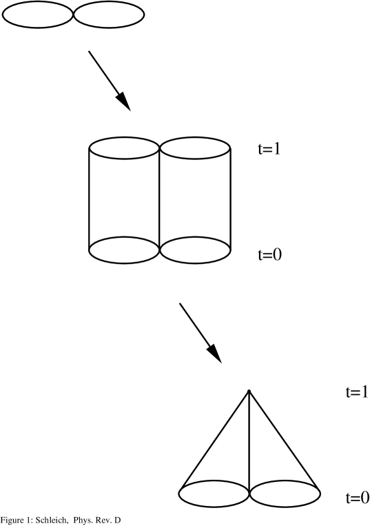
FIG. 1.: The construction of a cone of a topological space $V$. In this example, $V$ is a one dimensional space consisting of a figure eight as seen at upper left. The product space $V\times I$ is illustrated in the middle; it is a two dimensional space consisting of two cylinders with points identified on the line where they touch. The cone of $V$ constructed from this product space is illustrated at lower right; all points at $t=1$ are now identified to a single point.

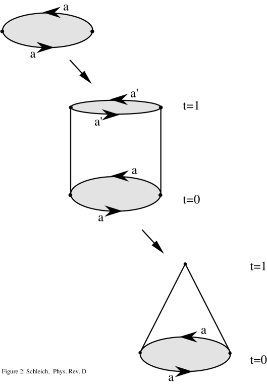
FIG. 2.: The construction of $C(RP^{2})$. In this construction, the space $RP^{2}$ is represented by a disk with antipodal points identified as seen at upper left. This representation and its connection with other representations of $RP^{2}$ is illustrated in Figure 3. The product space $RP^{2}\times I$ is illustrated in the middle. Note that the front surface of this three dimensional cylinder is identified with the back surface in accordance with the identification of the edges of $RP^{2}$. Thus this space is compact with two $RP^{2}$ boundaries. The cone $C(RP^{2})$ is again formed by identifying all points at $t=1$ to one point as illustrated at lower right. Observe that $C(RP^{2})$ has only one boundary, that of the base $RP^{2}$.

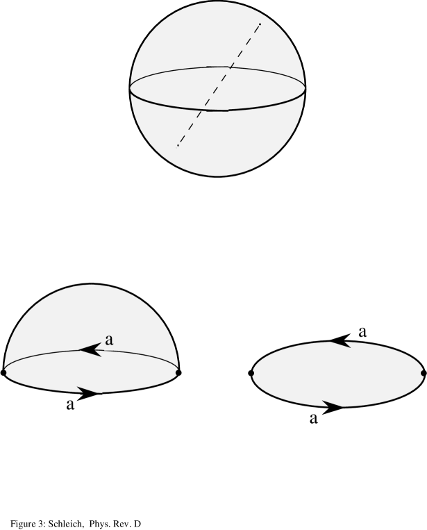
FIG. 3.: Constructions of $RP^{n}$. These constructions are explicitly illustrated for the case of $RP^{2}$. A familiar realization of $RP^{n}$ is given by the identification of antipodal points on $S^{n}$; explicitly embedding $S^{n}$ in ${\bf R}^{n+1}$, this identification is $x^{a}\to-x^{a}$ where $x^{a}$ is the cartesian coordinate of the point. The fundamental region of $RP^{n}$, that is the set of distinct points, is the upper hemisphere of $S^{n}$. The boundary of this region, the equator of the n-sphere, still has antipodal points identified; specifically, points on the front arc $a$ are identified with those on the back arc $a$ as indicated by the arrows. This representation of $RP^{n}$ is illustrated at lower left. As the hemisphere is homeomorphic to a n-ball, a topologically equivalent representation of $RP^{n}$ is given by a n-ball with antipodal points on its boundary identified as illustrated at lower right.

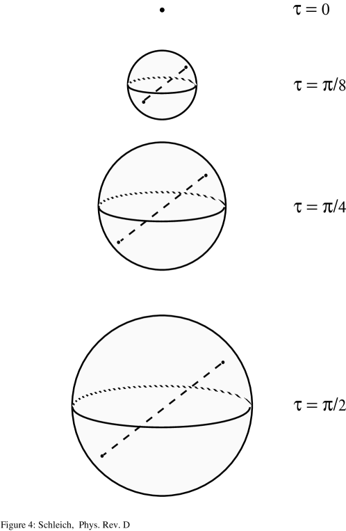
FIG. 4.: A representation of C($RP^{3}$). This four dimensional conifold cannot be explicitly drawn, but can be represented as a sequence of three dimensional slices. Each slice is $RP^{3}$ represented as a solid 3-ball with antipodal points on the surface identified as illustrated at lower right in Figure 3. The slice at $\tau=0$ consists of a single point.

REFERENCES

- [1] J. B. Hartle and S. W. Hawking, Phys. Rev. D 28, 2960 (1983).
- [2] S. W. Hawking, Nucl. Phys. B239, 257 (1984).
- [3] K. Schleich and D. M. Witt, Nucl. Phys. B402, 411 (1993).
- [4] K. Schleich and D. M. Witt, Nucl. Phys. B402, 469 (1993).
- [5] K. Schleich and D. M. Witt, in preparation.
- [6] J. B. Hartle in High Energy Physics 1985: Proceedings of the Yale Theoretical Advanced Study Institute ed. by M. J. Bowick and F. Gürsey (World Scientific, Singapore 1985) and J. B. Hartle, in Gravitation in Astrophysics: Proceedings of the 1986 Cargese NATO Summer Institute (World Scientific, Singapore 1987).
- [7] R. Laflamme, Phys. Lett. 198B, 156 (1987).
- [8] See for example, Michael Spivak, A Comprehensive Introduction to Differential Geometry, Vol 1 (Publish or Perish, Inc. Berkeley, 1979).
- [9] See for example p. 87, N. D. Birrell and P. C. W. Davies, Quantum Fields in Curved Space, (Cambridge University Press, 1982).
- [10] T. Banks, Nucl. Phys. B249, 332 (1985).
- [11] J. Cheeger, Proc. Natl. Acad. Sci. USA 96, No. 5, 2103 (1979).
- [12] Dmitri V. Fursaev, Sergey N. Solodukhin, Phys. Rev. D 52, 2133, (1995).
- [13] See for example, Chapter 8 in Handbook of Mathematical Functions M. Abramowitz and I. Stegun, eds. (Dover, New York, 1972).
- [14] There is a extensive literature on this issue, which is still unresolved. See for example, G.W. Gibbons, S. W. Hawking and M. J. Perry, Nucl. Phys. B138, 141 (1978), K. Schleich, Phys. Rev. D 36 2342 (1987) and Phys. Rev. D 39, 2192 (1989), and J. J. Halliwell and J. B. Hartle, Phys. Rev. D 41, 1815 (1990) for discussion of the issue and further references.
- [15] N. A. Chernikov and E. A. Tagirov, Ann. Inst. Henri Poincare 9, 109 (1968), E. A. Tagirov, Ann. Phys. 76, 561 (1973).
- [16] See for example, p. 134, N. D. Birrell and P. C. W. Davies, Quantum Fields in Curved Space, (Cambridge University Press, 1982).
- [17] See for example, E. M. Lifshitz and I. M. Khalatnikov, Ann. Phys. 12, 185, (1963).