Abstract

Recent work on state sum models of quantum gravity in 3 and 4 dimensions has led to interest in the ‘quantum tetrahedron’. Starting with a classical phase space whose points correspond to geometries of the tetrahedron in ${\mathbb{R}}^{3}$, we use geometric quantization to obtain a Hilbert space of states. This Hilbert space has a basis of states labeled by the areas of the faces of the tetrahedron together with one more quantum number, e.g. the area of one of the parallelograms formed by midpoints of the tetrahedron’s edges. Repeating the procedure for the tetrahedron in ${\mathbb{R}}^{4}$, we obtain a Hilbert space with a basis labelled solely by the areas of the tetrahedron’s faces. An analysis of this result yields a geometrical explanation of the otherwise puzzling fact that the quantum tetrahedron has more degrees of freedom in 3 dimensions than in 4 dimensions.

Introduction

State sum models for quantum field theories are constructed by giving amplitudes for the simplexes in a triangulated manifold. The simplexes are labelled with data from some discrete set, and the amplitudes depend on this labelling. The amplitudes are then summed over this set of labellings, to give a discrete version of a path integral. When the discrete set is a finite set, then the sum always exists, and so this procedure provides a bona fide definition of the path integral.

State sum models for quantum gravity have been proposed based on the Lie algebra ${\mathfrak{s}o}(3)$ and its $q$-deformation. Part of the labelling scheme is then to assign irreducible representations of this Lie algebra to simplexes of the appropriate dimension. Using the $q$-deformation, the set of irreducible representations becomes finite. However, we will consider the undeformed case here as the geometry is more elementary.

Irreducible representations of ${\mathfrak{s}o}(3)$ are indexed by a non-negative half-integers $j$ called spins. The spins have different interpretations in different models. In the Ponzano-Regge model of 3-dimensional quantum gravity [26], spins label the edges of a triangulated 3-manifold, and are interpreted as the quantized lengths of these edges. In the Ooguri-Crane-Yetter state sum model [11, 24], spins label triangles of a triangulated 4-manifold, and the spin is interpreted as the norm of a component of the $B$-field in a $BF$ Lagrangian [2]. There is also a state sum model of 4-dimensional quantum gravity in which spins label triangles [8]. Here the spins are interpreted as areas [8].

Many of these constructions have a topologically dual formulation. The dual 1-skeleton of a triangulated surface is a trivalent graph, each of whose edges intersect exactly one edge in the original triangulation. The spin labels can be thought of as labelling the edges of this graph, thus defining a spin network [3, 4, 25, 28]. In the Ponzano-Regge model, transition amplitudes between spin networks can be computed as a sum over labellings of faces of the dual 2-skeleton of a triangulated 3-manifold [15, 30]. Formulated this way, we call the theory a ‘spin foam model’.

A similar dual picture exists for 4-dimensional quantum gravity. The dual 1-skeleton of a triangulated 3-manifold is a 4-valent graph each of whose edges intersect one triangle in the original triangulation [21]. The labels on the triangles in the 3-manifold can thus be thought of as labelling the edges of this graph. The graph is then called a ‘relativistic spin network’. Transition amplitudes between relativistic spin networks can be computed using a spin foam model. The path integral is then a sum over labellings of faces of a 2-complex interpolating between two relativistic spin networks [5].

In this paper we consider the nature of the quantized geometry of a tetrahedron which occurs in some of these models, and its relation to the phase space of geometries of a classical tetrahedron in 3 or 4 dimensions. Our main goal is to solve the following puzzle: why does the quantum tetrahedron have fewer degrees of freedom in 4 dimensions than in 3 dimensions? This seeming paradox turns out to have a simple explanation in terms of geometric quantization. The picture we develop is that the four face areas of a quantum tetrahedron in four dimensions can be freely specified, but that the remaining parameters cannot, due to the uncertainty principle.

In the rest of this section we briefly review the role of the triangle in 3-dimensional quantum gravity and that of the tetrahedron in 4-dimensional quantum gravity. We also sketch the above puzzle and its solution. In the following sections we give a more detailed treatment.

0.1 The triangle in 3d gravity

In the Ponzano-Regge model, states are specified by labelling the edges of a triangulated surface by irreducible representations of ${\mathfrak{s}o}(3)$. Using ideas from geometric quantization, the spin-$j$ representation can be thought of as the Hilbert space of states of a quantized vector of length $j$. Once spins $j_{1},j_{2},j_{3}$ for the edges of a triangle are specified, a quantum state of the geometry of the triangle is an element

$$\psi\in j_{1}\otimes j_{2}\otimes j_{3}.$$

We require that this element satisfy a quantized form of the condition that the three edge vectors for a triangle sum to zero. The quantization of this condition is that $\psi$ be invariant under the action of ${\mathfrak{s}o}(3)$. As long as the spins satisfy the Euclidean triangle inequalities, there exists a unique element with this property, up to a constant factor. This reflects the fact that the geometry of a Euclidean triangle is specified entirely by its edge lengths. This unique invariant element is denoted graphically by the spin network

$${\raise 6.0pt\hbox{$j_{1}$}\atop\lower 6.0pt\hbox{$j_{2}$}}{\hbox to15.0pt{$\hfill$}\overwithdelims> .}\,j_{3}\,.$$

We call it a vertex because it corresponds to a vertex of the spin network dual to the triangulation.

The uniqueness of the vertex can be explained in terms of geometric quantization. This explanation serves as the prototype of the discussion below for the uniqueness of the vertex in the 4-dimensional model. Any irreducible representation of ${\mathfrak{s}o}(3)$ can be realised by an action of ${\rm SU}(2)$ on the space of holomorphic sections of some line bundle over $S^{2}$. Elements of the space $j_{1}\otimes j_{2}\otimes j_{3}$ thus correspond to holomorphic sections of the tensor product line bundle on $S^{2}\times S^{2}\times S^{2}$. A vertex therefore corresponds to an ${\rm SU}(2)$-invariant section of this tensor product line bundle.

In general, invariant holomorphic sections of a line bundle over a Kähler manifold correspond to sections of a line bundle over the symplectic reduction of this manifold by the group action [13]. Moreover, symplectic reduction eliminates degrees of freedom in conjugate pairs. Starting from the 6-dimensional manifold $S^{2}\times S^{2}\times S^{2}$ and reducing by the action of the 3-dimensional group ${\rm SU}(2)$, we are thus left with a 0-dimensional reduced space, since $6-3-3=0$.

In fact, when the spins $j_{i}$ satisfy the triangle inequality, the reduced space is just a single point. To see this, think of a point in $S^{2}\times S^{2}\times S^{2}$ as a triple of bivectors with lengths equal to $j_{1},j_{2},j_{3}$, respectively. The constraint generating the ${\rm SU}(2)$ action is that these bivectors sum to zero. When this constraint holds, the bivectors form a triangle in ${\mathfrak{s}o}(3)^{*}$ with edge lengths $j_{1},j_{2},j_{3}$. Since all such triangles are contained in one orbit of ${\rm SU}(2)$, the reduced phase space is a single point. This explains why the space of vertices is 1-dimensional: any vertex corresponds to a section of a line bundle over this point.

0.2 The tetrahedron in 4d gravity

A modification of the Ponzano-Regge model has been proposed to give a 4-dimensional state sum model of quantum gravity [8]. In these models states are described by labelling the triangles of a triangulated 3-manifold by irreducible representations of ${\mathfrak{s}o}(4)$. However, not all irreducible representations are allowed as labels, only certain ones called ‘balanced’ representations. This restriction can understood as follows.

In the Ponzano-Regge model, the basic idea was to describe triangles by labelling their edges with vectors in ${\mathbb{R}}^{3}$, and then to quantize this description. Similarly, in the 4-dimensional model we describe tetrahedra by labelling their faces with bivectors in ${\mathbb{R}}^{4}$, and then we quantize this description. A bivector in ${\mathbb{R}}^{4}$ is just an element of the second exterior power $\Lambda^{2}{\mathbb{R}}^{4}$. Given an oriented triangle in ${\mathbb{R}}^{4}$ we may associate to it the bivector formed as the wedge product of any two of its edges taken in cyclic order.

Irreducible representations of ${\mathfrak{s}o}(4)\cong{\mathfrak{s}o}(3)\oplus{\mathfrak{s}o}(3)$ are indexed by pairs of spins $(j,k)$. The $(j,k)$ representation can be thought of as the Hilbert space of states of a quantized bivector in 4 dimensions whose self-dual and anti-self-dual parts have norms $j$ and $k$, respectively. Classically, a bivector in ${\mathbb{R}}^{4}$ comes from a triangle as above if and only if its self-dual and anti-self-dual parts have the same norm. We impose this restriction at the quantum level by labelling triangles only with representations for which $j=k$. These are called balanced representations of ${\mathfrak{s}o}(4)$. When a triangle is labelled by the balanced representation $(j,j)$, the spin $j$ specifies its area. Thus in going from three to four dimensions, the geometric interpretation of a spin label changes from the length of an edge to the area of a triangle.

Having labelled its faces by balanced representations, the quantum state of the geometry of a tetrahedron in four dimensions is given by a vector

$$\psi\in(j_{1},j_{1})\otimes(j_{2},j_{2})\otimes(j_{3},j_{3})\otimes(j_{4},j_{4}).$$

As in the Ponzano-Regge model, we impose some conditions on this vector, motivated by the geometry of the situation. First, we require that this vector be invariant under the action of ${\mathfrak{s}o}(4)$. This is a quantization of the condition that the bivectors associated to the faces of a tetrahedron must sum to zero. Second, we require that given any pair of faces, e.g. 1 and 2, then in the decomposition

$$(j_{1},j_{1})\otimes(j_{2},j_{2})\cong\bigoplus_{j,k}(j,k)$$

the components of $\psi$ are zero except in the balanced summands, $(j,j)$. There are three independent conditions of this sort, one for the pair 1–2, one for the pair 1–3 and one for the pair 1–4. (Since the vector is invariant, the summands of the pair 3–4 which occur are exactly the same as for 1–2, and so on, so we do not need consider the other three pairs.) This quantizes the condition that any pair of faces of a tetrahedron must meet on an edge, geometrically a rather strong condition as a generic pair of planes in ${\mathbb{R}}^{4}$ meet at a point, not a line. Vectors $\psi$ meeting all these requirements are called vertices, now corresponding to the vertices of the 4-valent relativistic spin network dual to the triangulation of a 3-manifold.

Taking into account these conditions, the vertex is unique up to a constant factor. The formula for the vertex was given by Barrett and Crane [8], and an argument for its uniqueness was first given by Barbieri [7]. This argument depended on an assumption that some associated 6$j$-symbols do not have too many ‘accidental zeroes’. A simpler argument relying on the same assumption is given here. A proof of the uniqueness without any assumptions has been given by Reisenberger [27].

A basis for the invariant vectors is given by

$$B^{12}_{jk}={\raise 6.0pt\hbox{$j_{1}$}\atop\lower 6.0pt\hbox{$j_{2}$}}{\hbox to20.0pt{$\hfill j\hfill$}\overwithdelims> <{}}{\raise 6.0pt\hbox{$j_{3}$}\atop\lower 6.0pt\hbox{$j_{4}$}}\bigotimes{\raise 6.0pt\hbox{$j_{1}$}\atop\lower 6.0pt\hbox{$j_{2}$}}{\hbox to20.0pt{$\hfill k\hfill$}\overwithdelims> <{}}{\raise 6.0pt\hbox{$j_{3}$}\atop\lower 6.0pt\hbox{$j_{4}$}}.$$

Similar bases $B^{13}_{jk}$ and $B^{14}_{jk}$ are defined using the spin networks which couple the pairs 1–3 or 1–4 instead of 1–2. Any solution of the constraints for the quantum tetrahedron must be

$$\psi=\sum_{j}\lambda_{j}B^{12}_{jj}=\sum_{k}\mu_{k}B^{13}_{kk}=\sum_{l}\nu_{l}B^{14}_{ll}.$$ (1)

In other words, $\psi$ is a symmetric rank two tensor on the invariant subspace ${\rm Inv}(j_{1}\otimes j_{2}\otimes j_{3}\otimes j_{4})$ which is diagonal in three different bases. The change of basis matrix is, for each pair, a 6$j$-symbol. Since the 6$j$-symbol satisfies an orthogonality relation, there is a canonical solution to these constraints, given by taking $\psi$ to be (inverse of the) inner product in the orthogonality relation, $\lambda_{j}=(-1)^{2j}\dim j$. This gives the vertex described by Barrett and Crane [8].

Now suppose there is another solution $\lambda^{\prime}_{j}$. Then $\lambda^{\prime}_{j}/\lambda_{j}$ are the eigenvalues of a linear operator which is diagonal in each basis. It follows that the eigenspaces for each distinct eigenvalue are preserved under the change of basis, so the 6$j$-symbol must be zero for each choice of spin $j$ corresponding to one eigenvalue in $B^{12}_{jj}$ and spin $k$ corresponding to a different eigenvalue in $B^{13}_{kk}$. Assuming the 6$j$-symbol does not have accidental zeroes in this way, there cannot be two distinct eigenvalues, so the two solutions are just proportional to each other. Since accidental zeroes of the 6$j$ symbols are rather sparse [9], we expect the vertex to be unique — as was indeed shown by Reisenberger.

Still, from a geometrical viewpoint the uniqueness of the vertex is puzzling. After all, labelling a triangle with a balanced representation of ${\mathfrak{s}o}(4)$ only specifies the area of the triangle. Fixing the values of the areas of four triangles does not specify the geometry of a tetrahedron uniquely. The geometry of a tetrahedron is determined by its six edge lengths. Since the areas of the faces are only four parameters, there will be typically a 2-dimensional moduli space of tetrahedra with given face areas. Why then is a state of the quantum tetrahedron in four dimensions uniquely determined by the areas of its faces?

This puzzle is resolved here by developing a deeper understanding of the constraints, using geometric quantization. Essentially the issue is to understand the difference between a tetrahedron embedded in ${\mathbb{R}}^{3}$ and a tetrahedron embedded in ${\mathbb{R}}^{4}$. In classical geometry, these are not too different. In both cases we can describe the tetrahedron using bivectors for faces that sum to zero. But in the 4-dimensional situation there are also extra constraints implying that all four faces lie in a common hyperplane. When these are satisfied we are essentially back in the 3-dimensional situation.

Quantum mechanically, however, these extra constraints dramatically reduce the number of degrees of freedom for the tetrahedron. This is a standard phenomenon in quantum theory. A set of constraints introduced by operator equations

$$\widehat{H}_{i}\psi=0,\quad\quad i=1,\ldots,n$$

implies automatically that the quantum state vector $\psi$ is invariant under the group of symmetries generated by the set of operators $\widehat{H}_{i}$. The classical counterpart is symplectic reduction, or more generally Poisson reduction [22], in which one restricts the phase space to the subspace given by the constraints $H_{i}=0$, and then passes to the quotient space of orbits of the symmetry group generated by the constraints $H_{i}$.

Our explanation of the uniqueness of the vertex for the quantum tetrahedron in four dimensions is as follows. The Hilbert space

$$(j_{1},j_{1})\otimes(j_{2},j_{2})\otimes(j_{3},j_{3})\otimes(j_{4},j_{4})$$

corresponds to the classical phase space consisting of 4-tuples of simple bivectors having norms given by the four spins $j_{i}$. This phase space is 16-dimensional. The subspace of quantum states invariant under ${\mathfrak{s}o}(4)$ corresponds to the classical phase space of four such bivectors summing to zero, considered modulo the action of the rotation group ${\rm SO}(4)$ on all four bivectors simultaneously. This phase space is a 4-dimensional symplectic manifold (since $16-6-6=4$). The constraints (1) which force the triangles to intersect on edges are two independent equations. Symplectic reduction with two constraints reduces the 4-dimensional manifold to a 0-dimensional one (since $4-2-2=0$), in fact just a single point. This explains why the space of vertices is 1-dimensional.

This argument can also be phrased in terms of the uncertainty principle. There are two constraint equations $H_{i}=0$ that force the four faces of the tetrahedron to lie in a common hyperplane. These variables $H_{i}$ are canonically conjugate to the two variables determining the shape of a tetrahedron with faces of fixed area. Therefore by the uncertainty principle, the shape of the tetrahedron is maximally undetermined.

1 Quantum bivectors

By a bivector in $n$ dimensions we mean an element of $\Lambda^{2}{\mathbb{R}}^{n}$. A bivector records some of the information of the geometry of a triangle in ${\mathbb{R}}^{n}$. An oriented triangle has three edge vectors, $e,f,g$ which cycle around the triangle in that order. Then the bivector for the triangle is

$$E=e\wedge f=f\wedge g=g\wedge e.$$

These are equal due to the equation $e+f+g=0$. Therefore $b$ depends only on the triangle and its orientation, not on a choice of edges. The bivector determines a 2-dimensional plane in ${\mathbb{R}}^{n}$ with an orientation, and the norm of the bivector is twice the area of the triangle. However, no further details of the geometry of the triangle are recorded.

A bivector formed as the wedge product of two vectors is called simple. By the above remarks, we may think of any simple bivector as an equivalence class of triangles in ${\mathbb{R}}^{n}$. This interpretation becomes important in the next section, where we describe tetrahedra in terms of bivectors.

In three dimensions or below every bivector is simple, but this is not true in higher dimensions. For example, if $a_{1},a_{2},a_{3},a_{4}$ are linearly independent, then $a_{1}\wedge a_{2}+a_{3}\wedge a_{4}$ is not a simple bivector. In general, a bivector $E$ is simple if and only if $E\wedge E=0$. In four dimensions another criterion is also useful. The Euclidean metric and standard orientation on ${\mathbb{R}}^{4}$ determine a Hodge star operator

$$\ast\colon\Lambda^{2}{\mathbb{R}}^{4}\rightarrow\Lambda^{2}{\mathbb{R}}^{4}.$$

Since $\ast^{2}=1$, we may decompose any bivector into its self-dual and anti-self-dual parts:

$$E=E^{+}+E^{-},\qquad\ast E^{\pm}=\pm E^{\pm}.$$

The bivector is simple if and only if its self-dual and anti-self-dual parts have the same norm.

Using the Euclidean metric $\eta$ on ${\mathbb{R}}^{n}$ we may identify bivectors with elements of ${\mathfrak{s}o}(n)^{*}$. Explicitly, this isomorphism $\beta\colon\Lambda^{2}{\mathbb{R}}^{n}\rightarrow{\mathfrak{s}o}(n)^{\ast}$ is given by

$$\beta(e\wedge f)(l)=\eta(le,f)$$

for any bivector $e\wedge f$ and any $l\in{\mathfrak{s}o}(n)$. As recalled below, the dual of any Lie algebra has a natural Poisson structure. This allows us to treat the space of bivectors as a classical phase space. Using geometric quantization, we can quantize this phase space and construct a Hilbert space which we call the space of states of a ‘quantum bivector’. While this construction works in any dimension, we initially concentrate on dimension three. Then we turn to dimension four. In this case, the Hilbert space we construct has a subspace representing the states of a ‘simple’ quantum bivector.

1.1 Kirillov-Kostant Poisson structure

As shown by Kirillov and Kostant [18, 19], the dual of any Lie algebra ${\mathfrak{g}}$ is a vector space with an additional structure that makes it a Poisson manifold. This is a manifold with a Poisson bracket on its algebra of functions. We are mainly interested in the Lie algebra ${\mathfrak{s}o}(3)$ here, but ${\mathfrak{s}o}(4)$ is also important to us, so we briefly recall the general construction.

Elements $l,m$ of the Lie algebra determine linear functions on the dual vector space ${\mathfrak{g}}^{*}$. The Lie bracket $[l,m]$ can likewise be thought of as a function on ${\mathfrak{g}}^{*}$. This defines a Poisson bracket on the linear functions, and this extends uniquely to determine a Poisson bracket on the algebra of all smooth functions. Indeed, there is a bivector field $\Omega$ on the manifold ${\mathfrak{g}}^{*}$ such that

$$[l,m]=\Omega({\rm d}l,{\rm d}m)$$

Then the Poisson bracket in general is

$$\{f,g\}=\Omega({\rm d}f,{\rm d}g).$$

Since this formula is linear in ${\rm d}g$, it is given by the evaluation of ${\rm d}g$ on a vector field $f^{\#}$ on ${\mathfrak{g}}^{*}$

$$\{f,g\}={\rm d}g(f^{\#})=f^{\#}g.$$

In particular, each Lie algebra element $l$ determines a vector field $l^{\#}$. If $x\in{\mathfrak{g}}^{*}$, then the value of $l^{\#}m$ at $x$ is

$$(l^{\#}m)(x)=\langle x,[l,m]\rangle.$$

Thus if ${\mathfrak{g}}$ is the Lie algebra of a Lie group $G$, the vector fields $l^{\#}$ are given by the natural action of $G$ on ${\mathfrak{g}}^{*}$, the coadjoint action.

Coordinate formulae are sometimes illuminating for the above. Pick a basis $x^{i}$ for ${\mathfrak{g}}$, which gives coordinate functions on ${\mathfrak{g}}^{*}$. Then $[l,m]=[l_{i}x^{i},m_{j}x^{j}]=l_{i}m_{j}c^{ij}_{k}x^{k}$, where $c^{ij}_{k}$ are the structure constants of the Lie algebra. Then $\Omega^{ij}=c^{ij}_{k}x^{k}$, and $l_{\#}^{j}=l_{i}\Omega^{ij}$.

A 2-form $\omega$ is compatible with the Poisson structure if

$$\omega(l^{\#},m^{\#})=\{l,m\}.$$

This only determines $\omega$ on the span of the $l^{\#}$, namely the tangent space to the coadjoint orbit. Therefore, $\omega$ is defined as a 2-form on each orbit, called a symplectic leaf of the Poisson manifold. The Poisson bivector $\Omega$ is tangent to each leaf and non-degenerate as a bilinear form on the cotangent bundle of each leaf. The symplectic form $\omega$ is the inverse of this.

In the case of ${\mathfrak{s}o}(3)$, the Lie algebra can be identified with ${\mathbb{R}}^{3}$ with its standard vector cross product, the dual space can also be identified with ${\mathbb{R}}^{3}$, and then dual pairing $\langle\cdot,\cdot\rangle$ becomes the Euclidean inner product. Then

$$\{l,m\}(x)=\langle x,[l,m]\rangle$$

which looks the same as before, but now the right-hand side is the triple scalar product of vectors in ${\mathbb{R}}^{3}$. The 2-form is

$$\omega(a,b)={1\over x^{2}}\langle x,[a,b]\rangle.$$

In this case, the coadjoint action is the familiar action of rotations on the vector space of angular momenta, and so the symplectic leaves are spheres centered at the origin. The integral of $\omega$ over one of these spheres of Euclidean radius $r$ is $\pm 4\pi r$, the sign depending on the chosen orientation of the sphere. This differs from the Euclidean area due to the scaling factors in the formulae.

1.2 Quantization

Throughout this paper we quantize Poisson manifolds by constructing a Hilbert space for each symplectic leaf and then forming the direct sum of all these Hilbert spaces. We construct the Hilbert space for each leaf using geometric quantization, or more precisely, Kähler quantization [12, 29, 31]. For this we need to introduce some extra structure on each leaf. First we choose a complex structure $J$ on the leaf that preserves the symplectic form $\omega$, making the leaf into a Kähler manifold. Then we choose a holomorphic complex line bundle $L$ over the leaf, called the prequantum line bundle equipped with a connection whose curvature equals $\omega$:

$$\omega(\xi,\eta)s=i\left(\nabla_{\xi}\nabla_{\eta}-\nabla_{\eta}\nabla_{\xi}-\nabla_{[\xi,\eta]}\right)s.$$

For this, the symplectic leaf must be integral: the closed 2-form $\omega/2\pi$ must define an integral cohomology class. In this case, we define the Hilbert space for the leaf to be the space of square-integrable holomorphic sections of $L$. For nonintegral leaves, we define the Hilbert space to be 0-dimensional.

In the case of ${\mathfrak{s}o}(3)^{*}$, the integral symplectic leaves are the spheres centered at the origin for which the integral of $\omega$ is $2\pi$ times an integer. These are spheres $S_{j}$ with radii given by nonnegative half-integers $j$ — honest 2-spheres for $j>0$, and a single point for $j=0$. Each sphere $S_{j}$ with $j>0$ has a complex structure $J$ corresponding to the usual complex structure on the Riemann sphere. Explicitly, using the identification of ${\mathfrak{s}o}(3)^{\ast}$ and ${\mathfrak{s}o}(3)$, the formula for $J$ at a point $x$

$$J(a)={1\over|x|}[x,a].$$

In other words, $J$ rotates tangent vectors a quarter turn counter-clockwise. Clearly $J$ is a complex structure preserving the symplectic form $\omega$. The sphere thus becomes a Kähler manifold with Riemannian metric given by

$$g(a,b)=\omega(a,Jb)={1\over|x|}\langle a,b\rangle.$$

Like the symplectic structure itself, this differs from the standard induced metric by a scale factor.

When $j=0$, $S_{j}$ is trivially a Kähler manifold. In this case the prequantum line bundle is trivial and the Hilbert space of holomorphic sections is 1-dimensional. When $j={1\over 2}$, we may choose the prequantum line bundle to be the spinor bundle over $S_{j}$. The Hilbert space of holomorphic sections is then isomorphic to ${\mathbb{C}}^{2}$. For other values of $j$ we choose $L$ to be the $2j$th tensor power of the spinor bundle over $S_{j}$. The Hilbert space of holomorphic sections is then isomorphic to the $2j$th symmetrized tensor power $S^{n}{\mathbb{C}}^{2}$, which is $(2j+1)$-dimensional. We may associate to any Lie algebra element $l\in{\mathfrak{s}o}(3)$ a self-adjoint operator $\hat{l}$ on this Hilbert space, given by

$$\hat{l}\colon s\mapsto i\nabla_{l^{\#}}s-ls$$

On the right hand side, $l$ is regarded as a function on the coadjoint orbit, and multiplies the section $s$ pointwise. This formula gives a representation of ${\mathfrak{s}o}(3)$ which is just the usual spin-$j$ representation.

Taking the sum over all symplectic leaves, we obtain the Hilbert space of a quantum bivector in 3 dimensions,

$${\cal H}=\bigoplus_{j}j.$$

This is the basic building-block of all the more complicated quantized geometrical structures appearing in state sum models of quantum gravity [5]. Let $E^{i}$ be a basis of ${\mathfrak{s}o}(3)$ satisfying the Poisson bracket relations

$$\{E^{1},E^{2}\}=E^{3},\qquad\{E^{2},E^{3}\}=E^{1},\qquad\{E^{3},E^{1}\}=E^{2}.$$

when thought of as coordinate functions on ${\mathfrak{s}o}(3)^{\ast}$. Then by the above we obtain self-adjoint operators $\hat{E}^{i}$ on ${\cal H}$ satisfying the usual angular momentum commutation relations:

$$[\hat{E}^{1},\hat{E}^{2}]=i\hat{E}^{3},\qquad[\hat{E}^{2},\hat{E}^{3}]=i\hat{E}^{1},\qquad[\hat{E}^{3},\hat{E}^{1}]=i\hat{E}^{2}.$$

We think of these operators as observables measuring the 3 components of the quantum bivector. This interpretation is justified by the fact that these operators can also be obtained by geometrically quantizing the 3 coordinate functions on the space of bivectors. Their failure to commute means that the components of a quantum bivector cannot in general be measured simultaneously with complete precision.

1.3 The 4-dimensional case

In any dimension, starting from the Kirillov-Kostant Poisson structure on the dual of ${\mathfrak{s}o}(n)$, one can use geometric quantization to construct a Hilbert space describing the states of a quantum bivector. By the Bott-Borel-Weil theorem [10], this Hilbert space always turns out to be the direct sum of all the irreducible unitary representations of ${\mathfrak{s}o}(n)$. The 4-dimensional case is particularly simple, since we can reduce it to the previously treated 3-dimensional case using the isomorphism ${\mathfrak{s}o}(4)\cong{\mathfrak{s}o}(3)\oplus{\mathfrak{s}o}(3)$. This isomorphism corresponds to the splitting of a bivector into its self-dual and anti-self-dual parts.

Using this isomorphism, it follows that ${\mathfrak{s}o}(4)^{\ast}$ with its Kirillov-Kostant Poisson structure is the product of two copies of the Poisson manifold ${\mathfrak{s}o}(3)^{\ast}$. In particular, any symplectic leaf is of the form $S_{j}\times S_{k}$, that is, the product of a sphere of radius $j$ and a sphere of radius $k$, where $j,k$ are independent arbitrary spins. We can make this symplectic leaf into a Kähler manifold by taking the product of the previously described Kähler structures on $S_{j}$ and $S_{k}$. Similarly, we can equip the leaf with a line bundle given by the tensor product of the previously described line bundles over $S_{j}$ and $S_{k}$. As a result, when we geometrically quantize the leaf, we obtain a Hilbert space equal to the tensor product of the spin-$j$ representation of the ‘left-handed’ copy of ${\mathfrak{s}o}(3)$ and the spin-$k$ representation of the ‘right-handed’ copy. Taking the direct sum over all leaves, we thus obtain the Hilbert space

$${\cal H}\otimes{\cal H}=\bigoplus_{j,k}j\otimes k.$$

This is just the direct sum of all irreducible representations $(j,k)$ of ${\mathfrak{s}o}(4)$.

However, ${\mathfrak{s}o}(4)^{\ast}$ has another Poisson structure, obtained by reversing the sign of the Poisson structure on the anti-self-dual summand in ${\mathfrak{s}o}(3)^{\ast}\oplus{\mathfrak{s}o}(3)^{\ast}$. We call this the flipped Poisson structure. It turns out that the flipped Poisson structure is the right one for our purposes, as with this Poisson structure the quantum theory determines the chirality of the tetrahedron correctly, as is discussed in Section 3.2. The issue is to use the correct Poisson structure on $\Lambda^{2}{\mathbb{R}}^{4}$, which we identified with ${\mathfrak{s}o}(4)^{*}$ using the isomorphism $\beta$ described at the beginning of this section. We could achieve the same Poisson structure on $\Lambda^{2}{\mathbb{R}}^{4}$ by starting with the standard Poisson structure on ${\mathfrak{s}o}(4)^{*}$ and instead using the isomophism $\beta\circ\ast$, which differs by the Hodge dual $\ast$ acting on the bivectors. We return to this issue in Section 4.

With its flipped Poisson structure, ${\mathfrak{s}o}(4)^{\ast}$ again has integral symplectic leaves of the form $S_{j}\times S_{k}$; the only difference now is that the sign of the symplectic structure is reversed on $S_{k}$. We can thus make $S_{k}$ into a Kähler manifold with the Riemannian metric of the previous section but with the opposite complex structure. Proceeding as before, but with this modification, we can geometrically quantize ${\mathfrak{s}o}(4)^{\ast}$ and obtain the Hilbert space of a quantum bivector in 4 dimensions

$${\cal H}\otimes{\cal H}^{*}\cong\bigoplus_{j,k}j\otimes k^{*}$$

where starring stands for taking the complex conjugate Hilbert space, which is canonically isomorphic to the dual.

Using the splitting of ${\mathfrak{s}o}(4)^{*}$ into self-dual and anti-self-dual copies of ${\mathfrak{s}o}(3)^{*}$, we can put coordinate functions $E^{+i},E^{-i}$ on ${\mathfrak{s}o}(4)^{*}$ whose Poisson brackets with respect to the flipped Poisson structure are:

$$\{E^{+i},E^{+j}\}=\epsilon^{ijk}E^{+k},\qquad\{E^{-i},E^{-j}\}=-\epsilon^{ijk}E^{-k},\qquad\{E^{+i},E^{-j}\}=0.$$

The minus sign is the result of using the flipped Poisson structure. Using the recipe discussed in the previous section, we thus obtain self-adjoint operators $\hat{E}^{\pm i}$ on ${\cal H}\otimes{\cal H}^{*}$ satisfying the following commutation relations:

$$[{\hat{E}}^{+i},{\hat{E}}^{+j}]=i\epsilon^{ijk}{\hat{E}}^{+k},\qquad[{\hat{E}}^{-i},{\hat{E}}^{-j}]=-i\epsilon^{ijk}{\hat{E}}^{-k},\qquad[{\hat{E}}^{+i},{\hat{E}}^{-j}]=0.$$

As already noted, a bivector $b$ in 4 dimensions is simple if and only if its self-dual and anti-self-dual parts have the same norm. We may impose this constraint at the quantum level, obtaining the subspace of ${\cal H}\otimes{\cal H}^{*}$ consisting of states $\psi$ for which the Casimir operators

$$K^{\pm}=\sum_{k=1}^{3}(\hat{E}^{\pm k})^{2}$$

are equal:

$$K^{+}\psi=K^{-}\psi.$$

Alternatively, we may impose the constraint classically and then use geometric quantization to obtain a Hilbert space from the resulting Poisson manifold. Either way, we obtain the Hilbert space of a simple quantum bivector in 4 dimensions,

$$\bigoplus_{j}j\otimes j^{\ast}\;\subset\;{\cal H}\otimes{\cal H}^{*}.$$

2 The Quantum Tetrahedron in 3 Dimensions

A tetrahedron in ${\mathbb{R}}^{n}$ with labelled vertices, modulo translations, is determined by three vectors $e_{1},e_{2},e_{3}$, which are the edge vectors for three edges pointing out from a common vertex. The three triangular faces of the tetrahedron meeting at this vertex have bivectors

$$E_{1}=e_{2}\wedge e_{3},\;E_{2}=e_{3}\wedge e_{1},\;E_{3}=e_{1}\wedge e_{2},$$

while the bivector for the fourth face is

$$E_{4}=-E_{1}-E_{2}-E_{3}.$$

If the vectors $e_{i}$ are linearly dependent, then the $E$’s are all multiples of each other or zero. But in dimensions three or more, the vectors are generically linearly independent. From now on, we only consider this generic situation.

The map from triples of vectors to triples of bivectors is generically two-to-one, because if all three vectors are replaced by their negatives, then the bivectors are unchanged. Moreover, when the vectors $e_{i}$ are linearly independent, this operation is the only operation possible that changes the vectors but not the corresponding bivectors.

In dimension three, the map is also generically ‘half-onto’, in the sense that all positively oriented triples of bivectors $E_{1},E_{2},E_{3}$ arise, but never negatively-oriented ones. In three dimensions $\Lambda^{2}{\mathbb{R}}^{3}\cong{\mathbb{R}}^{3}$. With this identification the $\wedge$ operation is the vector cross product $\times$, so one can compute that

$$E_{1}\cdot(E_{2}\times E_{3})=V^{2}\geq 0$$

where $V=e_{1}\cdot(e_{2}\times e_{3})$ is 6 times the oriented volume of the tetrahedron. One also has

$$E_{1}\times E_{2}=Ve_{3}$$

etc., so that from a positively oriented triple $E_{1},E_{2},E_{3}$ one can compute the original $e$’s up to sign, i.e., obtaining either $(e_{1},e_{2},e_{3})$ or $(-e_{1},-e_{2},-e_{3})$. The distinction between these two triples of $e$’s is the orientation of the tetrahedron.

To summarise, a non-degenerate tetrahedron in 3 dimensions can be described by 4 bivectors, satisfying the closure constraint

$$E_{1}+E_{2}+E_{3}+E_{4}=0$$

together with the positivity constraint

$$E_{1}\cdot(E_{2}\times E_{3})>0.$$

The positivity constraint can be written in a number of equivalent ways by applying an even permutation to the 4 numbers $1234$. For example, the permutation $(14)(23)$ changes this formula to

$$E_{4}\cdot(E_{3}\times E_{2})>0$$

which is equivalent, using the closure constraint. Geometrically, the different formulae correspond to calculating $V^{2}$ using different vertices of the tetrahedron as the distinguished vertex.

2.1 Poisson structure

By the above we may describe a tetrahedron in 3 dimensions using a 4-tuple of bivectors $E_{1},\dots,E_{4}$ satisfying the closure and positivity constraints. In this section we think of these bivectors as elements of ${\mathfrak{s}o}(3)^{\ast}$. To obtain a Poisson structure on the space of geometries of a tetrahedron in 3 dimensions, we start by taking the product of 4 copies of ${\mathfrak{s}o}(3)^{\ast}$ with its Kirillov-Kostant Poisson structure, obtaining a Poisson structure on $({\mathfrak{s}o}(3)^{\ast})^{4}$. Then we perform Poisson reduction with respect to the closure constraint, as follows.

First we form the constraint submanifold

$$C=\{E_{1}+E_{2}+E_{3}+E_{4}=0\}\subset({\mathfrak{s}o}(3)^{\ast})^{4}.$$

The closure constraint generates the diagonal ${\rm SO}(3)$ action on $({\mathfrak{s}o}(3)^{\ast})^{4}$, which preserves $C$. To obtain the reduced space, we take the quotient of $C$ by this ${\rm SO}(3)$ action. We denote this quotient by $T$, and call it the phase space of a tetrahedron in 3 dimensions. Perhaps strictly speaking we should reserve this name for the subset of $T$ where the positivity constraint holds. However, this smaller phase space is hard to quantize, so it is more convenient to quantize all of $T$ and impose the positivity constraint at the quantum level. In fact, in applications to quantum gravity it may be best not to impose the positivity constraint at all. For more discussion of this issue see Section 4.

Any ${\rm SO}(3)$-invariant function on $({\mathfrak{s}o}(3)^{\ast})^{4}$ determines a function on $T$. We use this to define the following functions on $T$:

$$A_{i}=|E_{i}|,$$

$$A_{ij}=|E_{i}+E_{j}|,$$

and

$$U=E_{1}\cdot(E_{2}\times E_{3}).$$

These quantities have nice geometrical interpretations. The positivity constraint is $U>0$. Thus if $U>0$ there is a tetrahedron corresponding to the vectors $E_{i}$, while if $U<0$ there is a tetrahedron corresponding to the vectors $-E_{i}$. In either case, $|U|$ is 36 times the square of the volume of this tetrahedron. The quantity $A_{i}$ is twice the area of the $i$th face of the tetrahedron. Similarly, the quantity $A_{ij}$ is 4 times the area of the parallelogram with vertices given by the midpoints of the edges of the tetrahedron that are contained in either the $i$th or $j$th face of the tetrahedron, but not both. (See Fig. 1.) Alternatively, $A_{ij}$ is equal to $|u\wedge v|$, where $u$ is the displacement vector for the edge common to the $i$th and $j$th faces, and $v$ the displacement vector for the edge common to the other two faces.

As noted in our earlier work, these quantities satisfy some relations [5]. In particular, if $ijkl$ is any permutation of $1234$ we have

$$A_{ij}=A_{kl}.$$

We also have

$$A_{12}^{2}+A_{23}^{2}+A_{31}^{2}=A_{1}^{2}+A_{2}^{2}+A_{3}^{2}+A_{4}^{2}.$$

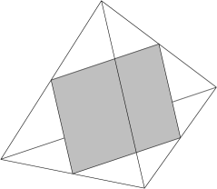
Figure 1: Parallelogram formed by midpoints of the tetrahedron’s edges

The map from ${\rm SO}(3)$-invariant functions on $({\mathfrak{s}o}(3)^{\ast})^{4}$ to functions on $T$ preserves Poisson brackets. Since the functions $|E_{i}|$ are constant on the symplectic leaves of $({\mathfrak{s}o}(3)^{\ast})^{4}$, it follows that the functions $A_{i}$ have vanishing Poisson brackets with all functions on $T$. The functions $A_{ij}$ do not. In particular, for any even permutation $ijkl$ of $1234$, we have

$$\{A_{ij}^{2},A_{ik}^{2}\}=4U.$$

When we quantize, this nonzero Poisson bracket leads to an uncertainty relation between the areas of the different parallelograms formed by midpoints of the tetrahedron’s edges. This is closely related to the ‘noncommutativity of area operators’ in loop quantum gravity [1], which has similar classical origins.

To prepare for geometric quantization, let us study the symplectic leaves of $T$. These are obtained from the leaves of $({\mathfrak{s}o}(3)^{\ast})^{4}$ by symplectic reduction with respect to the closure constraint. To visualize the situation it is best to think of the $E_{i}$ as vectors in ${\mathbb{R}}^{3}$. The constraint submanifold $C$ then consists of configurations of 4 vectors that close to form the sides of a (not necessarily planar) quadrilateral in ${\mathbb{R}}^{3}$. This description in terms of quadrilaterals allows us to apply the results of Kapovich, Millson [17], Hausmann and Knutson [16]. However, for the sake of a self-contained treatment we redo some of their work. Consider a symplectic leaf

$$\Lambda=\{|E_{i}|=r_{i}\}$$

in $({\mathfrak{s}o}(3)^{\ast})^{4}$. Its intersection with $C$ consists of all quadrilaterals with sides having fixed lengths $r_{1},\dots,r_{4}$. The corresponding leaf of $T$, namely $(\Lambda\cap C)/{\rm SO}(3)$, is thus the space of such quadrilaterals modulo rotations.

Generically, the leaves of $T$ are 2-spheres. In showing this, we shall exclude cases where ${\rm SO}(3)$ fails to act freely on $\Lambda\cap C$. These cases occur when $\Lambda\cap C$ contains a one-dimensional configuration, i.e., one in which the $E_{i}$ are all proportional to one another. This happens when $r_{1}+r_{2}=r_{3}+r_{4}$, $r_{1}=r_{2}+r_{3}+r_{4}$, or permutations of these. We shall also exclude cases where the quotient $(\Lambda\cap C)/{\rm SO}(3)$ is a single point. These cases occur when one or more of the $r_{i}$ vanish, and also when $r_{1}=r_{2}+r_{3}+r_{4}$ or permutations thereof.

Apart from these nongeneric cases, the leaf $(\Lambda\cap C)/{\rm SO}(3)$ is a 2-sphere. To see this, note first that the level sets of the function $A_{12}$ give a single point of this leaf at its maximum and minimum values. This is because at these points two of the $E_{i}$ are proportional, so the quadrilateral they form reduces to a triangle in ${\mathbb{R}}^{3}$. The triangle is rigid when its edge lengths are specified, so the set of such triangles modulo rotation is just one point. Next, note that when $A_{12}$ is neither a minimum or maximum, its level sets give circles in the leaf, parametrised by the angle $\theta$ between the plane spanned by $E_{1}$ and $E_{2}$ and the plane spanned by $E_{3}$ and $E_{4}$. (See Fig. 2.) It follows that the leaf is a 2-sphere.

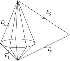
Figure 2: Circle formed by rotating $E_{1}$ and $E_{2}$ about $E_{1}+E_{2}$

On this 2-sphere, the meridians $\theta=0$ and $\theta=\pi$ correspond to quadrilaterals that lie in a plane in ${\mathbb{R}}^{3}$. In terms of tetrahedra, points on these meridians correspond to degenerate tetrahedra of zero volume, for which $U=0$. The two hemispheres $0<\theta<\pi$ and $\pi<\theta<2\pi$ correspond to the regions where $U>0$ and $U<0$. Which hemisphere corresponds to which sign of $U$ is a matter of convention in the definition of $\theta$. We can fix this convention by demanding that the Hamiltonian vector field generated by $A_{12}$ be $\partial_{\theta}$. The reason we can demand this is that $A_{12}$ generates rotations of the vectors $E_{1}$ and $E_{2}$ about the axis $E_{1}+E_{2}$, while leaving $E_{3}$ and $E_{4}$ fixed. With this convention $A_{12}$ and $\theta$ are canonically conjugate variables, so the symplectic structure on the 2-sphere is $\omega={\rm d}A_{12}\wedge{\rm d}\theta$.

2.2 Quantization

There are two strategies for constructing the space of states of the quantum tetrahedron in 3 dimensions. The first is to geometrically quantize $({\mathfrak{s}o}(3)^{\ast})^{4}$ and impose the closure constraint at the quantum level. The second is to impose the closure constraint at the classical level and geometrically quantize the resulting reduced space $T$. If the ${\rm SO}(3)$ action generated by the closure constraint were free, we could carry out both strategies and use a result of Guillemin and Sternberg [13] to show that they give naturally isomorphic vector spaces. In short, quantization would commute with reduction.

Unfortunately, as we saw in previous section, the ${\rm SO}(3)$ action generated by the closure constraint is not free. This complicates the second strategy. Generically ${\rm SO}(3)$ acts freely on the symplectic leaves of $({\mathfrak{s}o}(3)^{*})^{4}$, but there are also leaves on which the action is not free. In these nongeneric cases, the corresponding reduced leaf in $T$ has singular points where it is not a Kähler manifold. This presents an obstacle to geometric quantization.

With enough cleverness one could probably overcome this obstacle and generalize Guillemin and Sternberg’s result to cover this situation. Instead, we take a less ambitious approach. We carry out the first quantization strategy completely, carry out the second one for generic leaves of $({\mathfrak{s}o}(3)^{*})^{4}$, and show that the two strategies give naturally isomorphic vector spaces in the generic case.

In the first approach we start by geometrically quantizing $({\mathfrak{s}o}(3)^{\ast})^{4}$. Since geometric quantization takes products to tensor products, we obtain the Hilbert space ${\cal H}^{\otimes 4}$, where ${\cal H}$ is the Hilbert space of a quantum bivector in 3 dimensions, as defined in Section 1.2. Quantizing the coordinate functions $E_{1}^{i},\dots,E_{4}^{i}$ on $({\mathfrak{s}o}(3)^{\ast})^{4}$, we obtain operators $\hat{E}_{1}^{i},\dots,\hat{E}_{4}^{i}$ on ${\cal H}^{\otimes 4}$. Explicitly, we have

$$\hat{E}_{1}^{i}=\hat{E}^{i}\otimes 1\otimes 1\otimes 1$$

$$\hat{E}_{2}^{i}=1\otimes\hat{E}^{i}\otimes 1\otimes 1$$

$$\hat{E}_{3}^{i}=1\otimes 1\otimes\hat{E}^{i}\otimes 1$$

$$\hat{E}_{4}^{i}=1\otimes 1\otimes 1\otimes\hat{E}^{i}$$

where $i=1,2,3$. We then impose the closure constraint at the quantum level. This gives us the subspace of ${\cal H}^{\otimes 4}$ consisting of states $\psi$ with

$$(\hat{E}_{1}^{i}+\hat{E}_{2}^{i}+\hat{E}_{3}^{i}+\hat{E}_{4}^{i})\psi=0.$$

Such states are precisely those that are invariant under the action of ${\rm SU}(2)$. We call this subspace the Hilbert space of the quantum tetrahedron in 3 dimensions, and denote it by ${\cal T}$. Thus we have

$${\cal T}={\rm Inv}({\cal H}^{\otimes 4})\cong\bigoplus_{j_{1},\dots,j_{4}}{\rm Inv}(j_{1}\otimes\cdots\otimes j_{4})$$

where ‘Inv’ denotes the invariant subspace.

In the second approach, we start by noting that each integral symplectic leaf of $({\mathfrak{s}o}(3)^{\ast})^{4}$ is a product of 4 integral symplectic leaves of ${\mathfrak{s}o}(3)^{\ast}$. Thus it is of the form

$$\Lambda=\{|E_{i}|=j_{i}\}$$

for some spins $j_{1},\dots,j_{4}$. As a product of Kähler manifolds, it acquires the product Kähler structure. The closure constraint generates an ${\rm SO}(3)$ action which preserves this Kähler structure. As long as the spins $j_{i}$ do not satisfy $j_{1}+j_{2}=j_{3}+j_{4}$, $j_{1}=j_{2}+j_{3}+j_{4}$ or any permutations of these, this action is free. In this case, the reduced leaf $(\Lambda\cap C)/{\rm SO}(3)$ becomes a Kähler manifold as well. Geometrically quantizing this reduced leaf, we obtain a space of states. By the result of Guillemin and Sternberg, this vector space is naturally isomorphic to the space

$${\rm Inv}(j_{1}\otimes\cdots\otimes j_{4})\subset{\cal T}.$$

We can also see this last fact directly without using much machinery. The map from invariant states on $\Lambda$ to the state space for $(\Lambda\cap C)/{\rm SO}(3)$ is an injection. But we can see that these spaces have the same dimension, as follows. The dimension of the space of invariant states on $\Lambda$ is

$$\dim({\rm Inv}(j_{1}\otimes\cdots\otimes j_{4})=\min\{|j_{1}+j_{2}|,|j_{3}+j_{4}|\}-\max\{\left||j_{1}|-|j_{2}|\right|,\left||j_{3}|-|j_{4}|\right|\}+1$$

On the other hand, the Riemann-Roch theorem implies that the dimension of the state space for $(\Lambda\cap C)/{\rm SO}(3)$ is $1\over 2\pi$ times its symplectic volume plus 1. The symplectic volume was computed by Hausmann and Knutson [16] to be $2\pi(A_{\rm max}-A_{\rm min})$, where $A_{\rm min}$ and $A_{\rm max}$ are the minimum and maximum values of $A_{12}$. This is easy to see for generic leaves using the results of the previous section:

$$\int_{(\Lambda\cap C)/{\rm SO}(3)}\omega=\int_{A_{\rm min}}^{A_{\rm max}}\int_{0}^{2\pi}{\rm d}A_{12}\wedge{\rm d}\theta=2\pi(A_{\rm max}-A_{\rm min})$$

The dimension of the state space for $(\Lambda\cap C)/{\rm SO}(3)$ is thus $A_{\rm max}-A_{\rm min}+1$. But since $A_{12}=|E_{1}+E_{2}|=|E_{3}+E_{4}|$, we have

$$A_{\rm min}=\max\{\left||j_{1}|-|j_{2}|\right|,\left||j_{3}|-|j_{4}|\right|\},$$

$$A_{\rm max}=\min\{|j_{1}+j_{2}|,|j_{3}+j_{4}|\}.$$

Thus the two dimensions are equal.

The phase space discussed so far includes both genuine tetrahedra and their negatives, which do not satisfy the positivity constraint $U>0$. In a slightly different context, the implications of this issue for quantum gravity were addressed by Loll [20]. More recently, Barbieri [6] studied the obvious quantization of $U$, the Hermitian operator

$$\hat{U}=\sum_{i,j,k}\epsilon_{ijk}\hat{E}_{1}^{i}\hat{E}_{2}^{j}\hat{E}_{3}^{k},$$

He showed that if $u$ is an eigenvalue, so is $-u$. This arises because the natural antilinear structure map $P$ for representations of ${\rm SU}(2)$ acts on the quantum state space ${\cal T}$, and obeys the relations $P\hat{U}=-\hat{U}P$, $P^{2}=1$. Thus $P$ is a symmetry which interchanges eigenvectors of $U$ with opposite eigenvalues.

3 The Quantum Tetrahedron in 4 Dimensions

We now turn to the 4-dimensional case. As already noted, a tetrahedron in ${\mathbb{R}}^{4}$ with labelled vertices, modulo translations, is determined by 3 vectors $e_{1},e_{2},e_{3}$. Associating bivectors to the faces of the tetrahedron in the usual way:

$$E_{1}=e_{2}\wedge e_{3},\;E_{2}=e_{3}\wedge e_{1},\;E_{3}=e_{1}\wedge e_{2},$$

$$E_{4}=-E_{1}-E_{2}-E_{3},$$

we obtain a 4-tuple of simple bivectors $E_{1},\dots,E_{4}$ that sum to zero, with all their pairwise sums $E_{i}+E_{j}$ also being simple. The bivectors $E_{i}$ are simple because they come from triangles. Their pairwise sums are simple because these triangles lie in planes that pairwise span 3-dimensional subspaces of ${\mathbb{R}}^{4}$ — or equivalently, that intersect pairwise in lines.

As before, the map from the vectors $e_{i}$ to the bivectors $E_{i}$ is generically two-to-one: when the vectors $e_{i}$ are linearly independent, the $E_{i}$ uniquely determine the vectors $e_{i}$ up to sign. However, not every collection of simple bivectors $E_{1},\dots,E_{4}$ summing to zero with simple pairwise sums come from a tetrahedron this way. Generically there are 4 possibilities:

1. The bivectors $E_{i}$ come from a tetrahedron.

2. The bivectors $-E_{i}$ come from a tetrahedron.

3. The bivectors $\ast E_{i}$ come from a tetrahedron.

4. The bivectors $-\!\ast\!E_{i}$ come from a tetrahedron.

The proof is as follows. Recall that any nonzero simple bivector $e\wedge f$ determines a plane through the origin, namely that spanned by $e$ and $f$, and note that conversely, this plane determines the simple bivector up to a scalar multiple. Generically the bivectors $E_{1},E_{2},E_{3}$ are nonzero, and thus determine three planes $P_{1},P_{2},P_{3}\subset{\mathbb{R}}^{4}$. Since the pairwise sums of the $E_{i}$ are simple, these three planes generically intersect pairwise in lines. There are two cases:

• $P_{1}\cap P_{2}\neq P_{1}\cap P_{3}$. In this case $P_{1}$ is spanned by the lines $P_{1}\cap P_{2}$ and $P_{1}\cap P_{3}$. Thus it lies in the span of $P_{2}$ and $P_{3}$, which is a 3-dimensional subspace of ${\mathbb{R}}^{4}$. Since all three planes lie in this subspace, the problem reduces to the 3-dimensional case discussed in Section 2: either the bivectors $E_{i}$ come from a tetrahedron, or the bivectors $-E_{i}$ come from a tetrahedron.

• $P_{1}\cap P_{2}=P_{1}\cap P_{3}$. In this case all three planes $P_{i}$ share a common line, but generically they pairwise span three different subspaces, so the span of $P_{1}$ and $P_{2}$ differs from that of $P_{1}$ and $P_{3}$. Taking orthogonal complements, we thus have $P_{1}^{\perp}\cap P_{2}^{\perp}\neq P_{1}^{\perp}\cap P_{2}^{\perp}$. Thus all the hypotheses of the previous case hold, but with the planes $P_{i}$ replaced by the planes $P_{i}^{\perp}$. The planes $P_{i}^{\perp}$ correspond to the bivectors $\ast E_{i}$, so the argument in the previous case implies that either the bivectors $\ast E_{i}$ come from a tetrahedron, or $-\!\ast\!E_{i}$ come from a tetrahedron.

This proof makes no use of the bivector $E_{4}$, but of course the situation is perfectly symmetrical. If one forms planes corresponding to all 4 bivectors $E_{1},\dots,E_{4}$, one can check that in case (a), all 4 planes lie in the same 3-dimensional subspace of ${\mathbb{R}}^{4}$, while in case (b), all 4 planes contain the same line. The two cases are dual to each other in the sense of projective geometry.

One can easily distinguish between the cases 1-4 listed above using the self-dual and anti-self-dual parts $E_{i}^{\pm}$ of the bivectors $E_{i}$. Thinking of these bivectors as elements of ${\mathfrak{s}o}(4)$, we can define the quantities

$$U^{\pm}=\pm\langle E_{1}^{\pm},[E_{2}^{\pm},E_{3}^{\pm}]\rangle,$$

using the Killing form and Lie bracket in ${\mathfrak{s}o}(4)$. (Just as in 3 dimensions, we can equivalently define these quantities using any 3 of the bivectors $E_{1},\dots,E_{4}$.) Then cases 1-4 correspond to the following 4 cases, respectively:

1. $U^{+}>0,U^{-}<0$.

2. $U^{+}<0,U^{-}>0$.

3. $U^{+}>0,U^{-}>0$.

4. $U^{+}<0,U^{-}<0$.

Moreover, in all of these cases we have $|U^{+}|=|U^{-}|$. To prove this, we consider the 4 cases in turn:

1. If the bivectors $E_{i}$ come from a tetrahedron, there is a 3-dimensional subspace $V\subset{\mathbb{R}}^{4}$ such that all the $E_{i}$ lie in ${\mathfrak{s}o}(V)\subset{\mathfrak{s}o}(4)$. The results of Section 2 thus imply that $\langle E_{1},[E_{2},E_{3}]\rangle>0$. Note that we can choose a Lie algebra isomorphism $\alpha\colon{\mathfrak{s}o}(4)\rightarrow{\mathfrak{s}o}(3)\oplus{\mathfrak{s}o}(3)$ mapping ${\mathfrak{s}o}(V)$ to the ‘diagonal’ subalgebra consisting of elements of the form $(x,x)$. We can also choose $\alpha$ so that self-dual elements of ${\mathfrak{s}o}(4)$ are mapped to the first ${\mathfrak{s}o}(3)$ summand, while anti-self-dual elements are mapped to the second. Writing $\alpha(E_{i})=(x_{i},x_{i})$, we thus have

   $$\langle E_{1},[E_{2},E_{3}]\rangle=\langle(x_{1},x_{1}),[(x_{2},x_{2}),(x_{3},x_{3})]\rangle=2\langle x_{1},[x_{2},x_{3}]\rangle$$

   while

   $$U^{+}=\langle(x_{1},0),[(x_{2},0),(x_{3},0)]\rangle=\langle x_{1},[x_{2},x_{3}]\rangle$$

   and

   $$U^{-}=-\langle(0,x_{1}),[(0,x_{2}),(0,x_{3})]\rangle=-\langle x_{1},[x_{2},x_{3}]\rangle.$$

   It follows that $U^{+}>0$ and $U^{-}=-U^{+}$.

2. If the bivectors $-E_{i}$ come from a tetrahedron, since multiplying the $E_{i}$ by $-1$ reverses the sign of both $U^{+}$ and $U^{-}$, the above argument implies that $U^{+}<0$ and $U^{-}=-U^{+}$.

3. If the bivectors $\ast E_{i}$ come from a tetrahedron, since applying the Hodge star operator to the $E_{i}$ reverses the sign of $U^{-}$ but leaves $U^{+}$ unchanged, the above argument implies that $U^{+}>0$ and $U^{-}=U^{+}$.

4. Similarly, if the bivectors $-\!\ast\!E_{i}$ come from a tetrahedron, we have $U^{-}<0$ and $U^{-}=U^{+}$.

The remaining, non-generic, cases correspond to situations where both $U^{+}$ and $U^{-}$ vanish.

We may visualize the results of this section as follows. Suppose the bivectors $E_{1},\dots,E_{4}$ come from a nondegenerate tetrahedron $\tau$ in 4 dimensions. Then the bivectors $E_{i}^{+}$ come from a unique nondegenerate tetrahedron $\tau^{+}$ with positive oriented volume $\sqrt{U^{+}}$ in the 3-dimensional space of self-dual bivectors. Similarly, the $E_{i}^{-}$ come from a unique nondegenerate tetrahedron $\tau^{-}$ with positive oriented volume $\sqrt{-U^{-}}$ in the space of anti-self-dual bivectors. Since $|E_{i}^{+}|=|E_{i}^{-}|$ and $|E_{i}^{+}+E_{j}^{+}|=|E_{i}^{-}+E_{j}^{-}|$, the tetrahedra $\tau^{+}$ and $\tau^{-}$ differ only by a rotation. Conversely, any pair of tetrahedra $\tau^{+}$, $\tau^{-}$ with these properties determines a nondegenerate tetrahedron $\tau$ in 4 dimensions, unique up to the transformation $x\mapsto-x$.

3.1 Poisson structure

We obtain the phase space of the tetrahedron in 4 dimensions by starting with phase space of 4-tuples of bivectors and then imposing suitable constraints. The phase space of 4-tuples of bivectors is the product of 4 copies of ${\mathfrak{s}o}(4)^{\ast}$ with the ‘flipped’ Poisson structure described in Section 1.1. This space has coordinate functions $E^{\pm j}_{1},\dots,E^{\pm j}_{4}$ where $j=1,2,3$, satisfying the Poisson bracket relations:

$$\{E^{+j}_{i},E^{+k}_{i}\} = \epsilon^{jkl}E^{+l}_{i}$$

$$\{E^{-j}_{i},E^{-k}_{i}\} = -\epsilon^{jkl}E^{-l}_{i}$$

$$\{E^{+j}_{i},E^{-k}_{i}\} = 0$$

$$\{E^{\pm j}_{i},E^{\pm k}_{i^{\prime}}\} = 0\qquad i\neq i^{\prime}.$$

To obtain the phase space of a tetrahedron in 4 dimensions, we do Poisson reduction using the following constraints:

1. The closure constraint $E_{1}+E_{2}+E_{3}+E_{4}=0$.

2. The simplicity constraints $|E_{i}^{+}|^{2}=|E_{i}^{-}|^{2}$.

3. The simplicity constraints $|E_{i}^{+}+E_{j}^{+}|^{2}=|E_{i}^{-}+E_{j}^{-}|^{2}$.

4. The chirality constraint $U^{+}+U^{-}=0$.

The last constraint eliminates the fake tetrahedra of types 3 and 4, leaving genuine tetrahedra (type 1) and their negatives (type 2).

First we deal with the closure constraint. This is equivalent to separate closure constaints for the self-dual and anti-self-dual parts of the $E_{i}$:

$$E_{1}^{+}+\cdots+E_{4}^{+}=0,\qquad E_{1}^{-}+\cdots+E_{4}^{-}=0$$

Thus Poisson reduction by this constraint takes us from the 24-dimensional space $({\mathfrak{s}o}(4)^{\ast})^{4}$ down to 12-dimensional space $T^{+}\times T^{-}$, where $T^{+}$ is a copy of the phase space for a tetrahedron in 3 dimensions, and $T^{-}$ is another copy, but with minus the standard Poisson structure.

By the results of Section 2.1, the functions $|E_{i}^{\pm}|^{2}$ push down to smooth functions on $T^{+}\times T^{-}$, and the symplectic leaves of $T^{+}\times T^{-}$ are the sets on which all 8 of these functions are constant. Generically these leaves are of the form $S^{2}\times S^{2}$. The following functions also push down to smooth functions on $T^{+}\times T^{-}$:

$$C_{i}=|E_{i}^{+}|^{2}-|E_{i}^{-}|^{2},$$

$$C_{ij}=|E_{i}^{+}+E_{j}^{+}|^{2}-|E_{i}^{-}+E_{j}^{-}|^{2}.$$

The $C_{i}$ have vanishing Poisson brackets with every function on $T^{+}\times T^{-}$. The $C_{ij}$ do not, and in particular, taking $ijkl$ to be any even permutation of $1234$, we have

$$\{C_{ij},C_{ik}\}=4(U^{+}+U^{-}).$$

Next we deal with the simplicity constraints $C_{i}=0$. Since the $C_{i}$ have vanishing Poisson brackets with every function, they generate trivial flows, so in this case Poisson reduction merely picks out the 8-dimensional subspace

$$\{C_{i}=0\}\subset T^{+}\times T^{-}.$$

A point $(t^{+},t^{-})$ of $T^{+}\times T^{-}$ corresponds to a pair of tetrahedra or negative tetrahedra modulo rotations in 3 dimensions. When we refer to $t^{+}$, for example, as a tetrahedron, this means the geometrical tetrahedron formed either by the vectors $t^{+}$ if $U^{+}\geq 0$ or that formed by $-t^{+}$ if $U^{+}\leq 0$.

A point in the subspace $\{C_{i}=0\}$ corresponds to such a pair whose corresponding faces have equal areas. The symplectic leaves $L$ of this subspace are again generically of the form $S^{2}\times S^{2}$, and consist of the pairs of tetrahedra in 3 dimensions for which the common values for their four face areas are constants. Recall that each $S^{2}$ is divided into two hemispheres on which $U\geq 0$ and $U\leq 0$. The equator $\{U=0\}$ is the circle of degenerate tetrahedra.

Now we consider the simplicity constraints $C_{ij}=0$ and the chirality constraint $U^{+}+U^{-}=0$. On the subspace $\{C_{i}=0\}$ only two of the constraints $C_{ij}=0$ are independent, since for any permutation $ijkl$ of $1234$ we have

$$C_{ij}=C_{kl},$$

and we also have

$$C_{12}+C_{23}+C_{31}=C_{1}+C_{2}+C_{3}+C_{4}.$$

Thus the subspace

$$\{C_{i}=C_{ij}=0\}\subset T^{+}\times T^{-}$$

is generically 6-dimensional. To describe its structure, it is easiest to consider its intersection with a particular symplectic leaf $L$.

The constraints $C_{ij}=0$ imply that the two tetrahedra $t^{+},t^{-}$ are isometric. Then $t^{+}=t^{-}$ or $t^{+}=-{t}^{-}$, and these are both true if and only if $U^{+}=U^{-}=0$. This means that the constraints are satisfied on two copies of $S^{2}$ embedded in $L$ which intersect in the circle $\{U^{+}=U^{-}=0\}$. These embedded spheres, which we denote by $X$ and $\bar{X}$, satisfy the equations $U^{+}+U^{-}=0$ and $U^{+}-U^{-}=0$ respectively.

The surfaces $X$ and $\bar{X}$ differ markedly with respect to the symplectic structure. It is worth comparing the situation with the Kähler reduction by a group action. In the latter, the reduced phase space is the space of orbits of the group action in the constraint surface. The constraint surface is coisotropic, i.e., the tangent space contains its symplectic complement, and the tangents to the orbits are in this symplectic complement. This means that if $v$ is tangent to the orbit and $u$ is tangent to the constraint surface, then $\omega(v,u)=0$. The wavefunctions which are invariant under the group action localise to a small region around the constraint surface and are determined by their values on it.

The situation we have here with the constraints $C_{ij}=0$ differs in that they do not form a Lie algebra. However $X$ is coisotropic (in fact Lagrangian) and the fact that the commutator of two of the $C_{ij}$ vanishes on $X$ implies that the Hamiltonian vector fields they generate are tangent to $X$. Thus the situation is in most respects similar to the group case. On the other hand, $\bar{X}$ is not coisotropic, and the Hamiltonian vector fields are not tangent to it. Thus there is no sensible reduction procedure for wavefunctions based on $\bar{X}$.

3.2 Quantization

Finally, let us quantize the tetrahedron in 4 dimensions. As in 3 dimensions, there are two strategies. The first is to geometrically quantize $({\mathfrak{s}o}(4)^{\ast})^{4}$ and impose the closure, simplicity and chirality constraints at the quantum level. The second is to impose these constraints at the classical level and geometrically quantize the resulting reduced space. As we have already seen, there is a problem with the second approach: the simplicity constraints $C_{ij}$ do not generate a Lie group action on the symplectic leaf $L$. Thus we can only carry out the second strategy in a rather ad hoc way. If we do so, we obtain a 1-dimensional space of states for each generic integral leaf $L$. In some sense this explains the uniqueness of the vertex. Unfortunately, we cannot apply the results of Guillemin and Sternberg to rigorously conclude that the first strategy also gives a 1-dimensional state space for a tetrahedron with faces of fixed area.

In the first strategy, we start by geometrically quantizing the product of four copies of ${\mathfrak{s}o}(4)^{\ast}$ with its flipped Poisson structure. By the results of Section 1.2 we obtain the Hilbert space $({\cal H}\otimes{\cal H}^{\ast})^{\otimes 4}$, together with operators $\hat{E}_{i}^{\pm j}$ on this space which satisfy the following commutation relations:

$$[{\hat{E}_{i}}^{+j},{\hat{E}_{i}}^{+k}] = i\epsilon^{jkl}{\hat{E}_{i}}^{+l}$$

$$[{\hat{E}_{i}}^{-j},{\hat{E}_{i}}^{-k}] = -i\epsilon^{jkl}{\hat{E}_{i}}^{-l}$$

$$[{\hat{E}_{i}}^{+j},{\hat{E}_{i}}^{-k}] = 0$$

$$[{\hat{E}_{i}}^{\pm j},{\hat{E}_{i^{\prime}}}^{\pm k}] = 0\qquad i\neq i^{\prime}.$$

Geometrically quantizing the closure constraint we obtain the operators

$$\hat{E}_{1}^{\pm}+\cdots+\hat{E}_{4}^{\pm},$$

while quantizing the simplicity constraints gives the operators

$$\hat{C}_{i}=\sum_{k=1}^{3}(\hat{E}^{k}_{i})^{2},\qquad\hat{C}_{ij}=\sum_{k=1}^{3}(\hat{E}^{k}_{i}+\hat{E}^{k}_{j})^{2}.$$

The states annihilated by the quantized closure constraint form the subspace

$${\cal T}\otimes{\cal T}^{\ast}\subset({\cal H}\otimes{\cal H}^{\ast})^{\otimes 4}$$

where ${\cal T}\subset{\cal H}^{\otimes 4}$ is the Hilbert space of the quantum tetrahedron in 3 dimensions. Among these states, those that are also annihilated by the simplicity constraints $\hat{C}_{i}$ form the subspace

$$\bigoplus_{j_{1},j_{2},j_{3},j_{4}}{\rm Inv}((j_{1},j_{1})\otimes\cdots\otimes(j_{4},j_{4}))\subset{\cal T}\otimes{\cal T}^{*}.$$

The operators $\hat{C}_{ij}$ map each of these summands to itself, and as shown by Reisenberger [27], each nonzero summand has a 1-dimensional subspace that is annihilated by all these operators. We call the direct sum of all these 1-dimensional spaces the Hilbert space of the quantum tetrahedron in four dimensions.

The reader may wonder why we have not dealt with the chirality constraint. If we geometrically quantize this constraint we obtain the operator $\hat{U}^{+}+\hat{U}^{-}$, where

$$\hat{U}^{\pm}=\sum_{i,j,k}\epsilon_{ijk}\,\hat{E}_{1}^{\pm i}\,\hat{E}_{2}^{\pm j}\,\hat{E}_{3}^{\pm k}.$$

Barbieri [7] has shown that

$$4i[\hat{C}_{ij},\hat{C}_{ik}]=\hat{U}^{+}+\hat{U}^{-}.$$

Thus any solution $\psi$ of the simplicity constraints automatically satisfies the chirality constraint

$$(\hat{U}^{+}+\hat{U}^{-})\psi=0.$$

In other words, fake tetrahedra of types 3 and 4 do not occur in the quantum theory.

In the second strategy, we attempt to impose all the constraints at the classical level and then quantize. We did most of the work for this in the previous section. Starting from $({\mathfrak{s}o}(4)^{\ast})^{4}$ and doing symplectic reduction using the closure constraint, we obtained the space $T^{+}\times T^{-}$. Imposing the simplicity constraints $C_{i}=0$ we obtained an 8-dimensional space with symplectic leaves $L$ generically of the form $S^{2}\times S^{2}$. Recall that any point in $L$ corresponds to a pair $(t^{+},t^{-})$ of tetrahedra in 3 dimensions (modulo rotations) such that the $i$th face of both $t^{+}$ and $t^{-}$ has area $j_{i}$. If at this stage we geometrically quantized an integral generic leaf $L$, we would obtain the Hilbert space of states

$${\rm Inv}((j_{1},j_{1})\otimes\cdots\otimes(j_{4},j_{4})),$$

which is one of the summands mentioned above. We could then impose the remaining simplicity constraints at the quantum level as before. However, let us impose the simplicity constraints $C_{ij}=0$ at the classical level. We obtain a union of two spheres $X\cup\bar{X}$. The chirality constraint holds only on $X$, so we restrict attention to this space.

As already noted, the constraints $C_{ij}$ do not generate a Lie group action on $L$. However, they generate flows that act transitively on the sphere $X$, in the sense that all smooth functions invariant under all these flows are constant on $X$. Thus we may say, in a somewhat ad hoc way, that the symplectic reduction of the leaf $L$ by the constraints $C_{ij}$ is a single point. Geometrically quantizing this point, we obtain a 1-dimensional space of states, in accord with Reisenberger’s result. Alternatively, we may think of this 1-dimensional space as the space of constant functions on $X$. This makes the uniqueness of the vertex much less mysterious.

Unfortunately, we cannot use this to give a new proof of Reisenberger’s result, because we do not know that quantization commutes with reduction in this case. The reason is that the constraints $C_{ij}$ do not generate a Lie group action on $L$. Moreover, the flows they generate do not preserve the Kähler structure on $L$. A complete proof of the uniqueness of the vertex using geometrical quantization will apparently require new ideas. Flude has studied some similar constraints which give results in this direction which hold in the asymptotic limit of large spin [14].

4 Considerations from Quantum Gravity

The action for Riemannian general relativity in 4 dimensions, expressed in terms of a linear connection and an ${\mathbb{R}}^{4}$-valued one-form $e$, can be written as:

$$\int\langle F,*(e\wedge e)\rangle$$

where $F$ is the ${\mathfrak{s}o}(4)$-valued 2-form giving the curvature, $e\wedge e$ is the induced bivector-valued 2-form, and $*$ the Hodge star. The brackets $\langle\cdot\,,\cdot\rangle$ denote the standard pairing of ${\mathfrak{s}o}(4)$ with $\Lambda^{2}{\mathbb{R}}^{4}$ introduced in section 1, extended to differential forms by using the exterior product of forms. The inner product $\langle\cdot\,,\ast\,\cdot\rangle$ is exactly the one that leads to the flipped Poisson structure we introduced. This means that the Poisson structure we introduced so that the quantization leads to real tetrahedra, and not fake tetrahedra, is exactly the one relevant for the quantization of the Einstein action.

A further issue is the negative tetrahedra, the ones of type 2 for which the bivectors $-E$ come from a tetrahedron. These configurations make up half of the phase space $X$. There is a classical symmetry $E\mapsto-E$, and a corresponding quantum operator, $P\otimes P$, with $P$ the antilinear operator discussed in Section 2.2. Since this commutes with the quantum constraints, $(P\otimes P)\psi=c\psi$, with $c$ a complex number of unit modulus. The interpretation of this is that the quantum tetrahedron in four dimensions contains both tetrahedra and negative tetrahedra in equal measure. It does not seem that one can easily exclude the negative tetrahedra. There is a natural interpretation which may provide an explanation. One can change the sign of the isomorphism $\beta\colon\Lambda^{2}{\mathbb{R}}^{n}\rightarrow{\mathfrak{s}o}(n)^{\ast}$ by replacing the Euclidean metric $\eta$ by $-\eta$. Thus the negative tetrahedra have an interpretation as genuine tetrahedra for the opposite signature of the space-time metric.

Finally, there remains the question of the implication of our results to the nature of quantum geometry. An approach based on areas is in many ways a natural extension of 3-dimensional quantum gravity based on lengths. However it differs rather substantially from a naive expectation of a 4-dimensional approach based on lengths. As we have seen, a quantum tetrahedron does not appear to have a unique metric geometry. This means that in a state-sum approach based on gluing 4-simplexes together across a common tetrahedron, as outlined in [8], the metric of the tetrahedron does not transmit across from one 4-simplex to another. Rather, the parallelogram areas are randomised as one crosses from one 4-simplex to another. As we have shown here, this is a direct consequence of the uncertainty principle.

Acknowledgments

We would like to thank Andrea Barbieri, Laurent Freidel, Allen Knutson, Kirill Krasnov, Michael Reisenberger, Alan Weinstein, and José-Antonio Zapata for useful discussions and correspondence. In particular, we thank Zapata for pointing out the importance of the flipped Poisson structure.

References

- [1] A. Ashtekar, A. Corichi and J. Zapata, Quantum theory of geometry III: Non-commutativity of Riemannian structures, preprint available as gr-qc/9806041.
- [2] J. Baez, Four-dimensional theory as a topological quantum field theory, Lett. Math. Phys. 38 (1996), 129-143.
- [3] J. Baez, Spin networks in gauge theory, Adv. Math. 117 (1996), 253-272.
- [4] J. Baez, Spin networks in nonperturbative quantum gravity, in The Interface of Knots and Physics, ed. L. Kauffman, American Mathematical Society, Providence, Rhode Island, 1996.
- [5] J. Baez, Spin foam models, Class. Quantum Grav. 15 (1998), 1827-1858.
- [6] A. Barbieri, Quantum tetrahedra and simplicial spin networks, Nucl. Phys. B518 (1998) 714-728.
- [7] A. Barbieri, Space of the vertices of relativistic spin networks, preprint available as gr-qc/9709076.
- [8] J.W. Barrett and L. Crane, Relativistic spin networks and quantum gravity, preprint available as gr-qc/9709028.
- [9] L. Biedenharn and J. Louck, Angular Momentum in Quantum Physics: Theory and Applications, Addison-Wesley, Reading, Massachusetts, 1981.
- [10] R. Bott, Homogeneous vector bundles, Ann. Math. 66 (1957), 203-248.
- [11] L. Crane and D. Yetter, A categorical construction of 4d TQFTs, in Quantum Topology, eds. L. Kauffman and R. Baadhio, World Scientific, Singapore, 1993.
- [12] V. Guillemin and S. Sternberg, Geometric Asymptotics, American Mathematical Society, Providence, Rhode Island, 1977.
- [13] V. Guillemin and S. Sternberg, Geometric quantization and multiplicities of group representations, Invent. Math. 67 (1982), 515-538.
- [14] J. P. M. Flude, Geometric Asymptotics of Spin. PhD thesis, University of Nottingham, 1998.
- [15] B. Hasslacher and M. Perry, Spin networks are simplicial quantum gravity, Phys. Lett. B103 (1981), 21-24.
- [16] J.-C. Hausmann and A. Knutson, Polygon spaces and Grassmannians, L’Enseignment Mathematique 43 (1997), 173-198.
- [17] M. Kapovich and J. Millson, The symplectic geometry of polygons in Euclidean space, Jour. Diff. Geom. 44 (1996) 479-51.
- [18] A. Kirillov, Elements of the Theory of Representations, Springer-Verlag, New York, 1976.
- [19] B. Kostant, Quantization and unitary representations, in Modern Analysis and Applications, Springer Lecture Notes in Mathematics, No. 170, Springer-Verlag, New York, 1970, pp. 87-207.
- [20] R. Loll, Imposing in discrete quantum gravity, Phys. Lett. B399 (1997), 227-232.
- [21] F. Markopoulou, Dual formulation of spin network evolution, preprint available as gr-qc/9704013.
- [22] J. Marsden and T. Ratiu, Reduction of Poisson manifolds, Lett. Math. Phys. 11 (1986), 161-169.
- [23] J. P. Moussouris, Quantum models of space-time based on recoupling theory, Ph.D. thesis, Department of Mathematics, Oxford University, 1983.
- [24] H. Ooguri, Topological lattice models in four dimensions, Mod. Phys. Lett. A7 (1992) 2799-2810.
- [25] R. Penrose, Angular momentum: an approach to combinatorial space-time, in Quantum Theory and Beyond, ed. T. Bastin, Cambridge U. Press, Cambridge, 1971.
- [26] G. Ponzano and T. Regge, Semiclassical limit of Racah coefficients, in Spectroscopic and Group Theoretical Methods in Physics, ed. F. Bloch, North-Holland, New York, 1968.
- [27] M. Reisenberger, On relativistic spin network vertices, preprint available as gr-qc/9809067.
- [28] C. Rovelli and L. Smolin, Spin networks in quantum gravity, Phys. Rev. D52 (1995), 5743-5759.
- [29] J. Snyatycki, Geometric Quantization and Quantum Mechanics, Springer-Verlag, New York, 1980.
- [30] V. Turaev and O. Viro, State sum invariants of 3-manifolds and quantum symbols, Topology 31 (1992), 865-902.
- [31] N. Woodhouse, Geometric Quantization, Oxford U. Press, Oxford, 1992.