Quantum interest for scalar fields in Minkowski spacetime

Frans Pretorius

Department of Physics and Astronomy
University of Victoria
P.O. Box 3055 STN CSC
Victoria B.C., Canada V8W 3P6

The quantum interest conjecture of Ford and Roman states that any negative energy flux in a free quantum field must be preceded or followed by a positive flux of greater magnitude, and the surplus of positive energy grows the further the positive and negative fluxes are apart. In addition, the maximum possible separation between the positive and negative energy decreases the larger the amount of negative energy. We prove that the quantum interest conjecture holds for arbitrary fluxes of non-interacting scalar field energy in 4D Minkowski spacetime, and discuss the consequences in attempting to violate the second law of thermodynamics using negative energy. We speculate that quantum interest may also hold for the Electromagnetic and Dirac fields, and might be applied to certain curved spacetimes.

1 Introduction

Quantum field theory permits the existence of states where the renormalized energy density can become arbitrarily negative in regions of spacetime even though the total energy is always positive [1]. Negative energy is an essential ingredient in many bizarre effects, including wormholes [2], warp drives [3], time machines [4]; and may be used to violate the $2^{nd}$ law of thermodynamics [5], [6]. Fortunately (or unfortunately!) there appear to be severe restrictions on the magnitude and duration of negative energies that might occur in a quantum field. One form of these restrictions are the “quantum inequalities”, originally proposed by Ford and Roman [7], [8] and studied by numerous authors since [9], which essentially state that large amounts of negative energy can only be “seen” for very short intervals of time. These inequalities have been used to place stringent limitations on warp drive and wormhole geometries [10],[11].

Recently, Ford and Roman proposed the “quantum interest conjecture” and proved it for delta function pulses of negative energy for massless scalar fields in 2D and 4D Minkowski spacetime [12]. This conjecture is a consequence of the quantum inequalities (QI’s), and states that any negative energy pulse (the “loan”) must be accompanied (“repaid”) by a positive energy pulse within a certain maximum time interval, and the larger the separation of the pulses the larger the magnitude the positive pulse must be relative to the negative pulse (i.e., repaid with “interest”). At first glance this statement may not seem too profound – after all the total energy must be positive, so if there is a location with negative energy there will be compensating positive energy somewhere in the spacetime. But the quantum interest conjecture tells us a lot more about the nature of negative energies in free-fields: negative energy is always in close proximity to an entourage of positive energy. This, for instance, has immediate consequences in attempts to violate the $2^{nd}$ law of thermodynamics. For suppose negative energies were “substantial” enough that one could in principle reflect only the negative energy part of the flux produced by an accelerating mirror as shown in Figure 1 (a variant of a device first proposed by Davies [6] who used it to construct a reversible process that effectively transferred energy from a cold body to a hot one without doing work). The resultant stream of negative energy could be sent far enough away from the device so that one could reasonably apply the free-field quantum inequalities to the stream. Even though each pulse within the stream may be consistent with the original quantum inequality, the stronger quantum interest conjecture strictly forbids such a flux of negative energy. This implies that the mirror device in Figure 1 cannot exist; if we want to reflect negative energy we must reflect its support of positive energy, which is at least as large in magnitude. Thus one cannot subject a hot body to a pure flux of negative energy to lower its entropy (at least using scalar quantum fields), as suggested in [6].

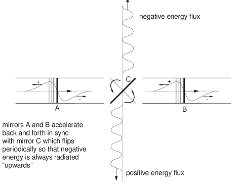
Figure 1: A pair of mirrors (A and B) accelerate back and forth in tandem, radiating negative energy in the direction of increasing acceleration and positive energy in the opposite direction. Between these two mirrors is a third mirror (C) that periodically flips so that the negative energy parts of the flux generated by mirrors A and B are always reflected in the same direction. Such a device could in principle produce a steady flow of negative energy, if it were possible to reflect just the negative part of the mirror flux.

In this paper, using a simple scaling argument, we present a proof of quantum interest for arbitrary distributions of negative energy of scalar fields in 4D Minkowski spacetime (slightly weaker results are obtained in 2D Minkowski spacetime). We do this first for the massless scalar field in section 3, after introducing the quantum inequalities in section 2. In section 4 we show that a massive scalar field has stronger constraints on the magnitude and duration of negative energies than a massless field, thus making the results of section 3 applicable to both types of scalar field. In section 5 we briefly comment on the possibility of extending quantum interest to the Electromagnetic and Dirac fields, curved spacetimes and to situations in Minkowski space where mirror-like boundary conditions are imposed on the fields.

2 Quantum inequalities

The quantum inequalities can be stated as follows. An inertial observer samples the local energy density $\rho(t)$ over a period of time with a sampling function $g(t)$ to obtain an average energy density $\langle\rho\rangle$:

$$\langle\rho\rangle=\int_{-\infty}^{\infty}g(t)\rho(t)dt.$$ (1)

The only conditions imposed upon $g(t)$ are that

$$\int_{-\infty}^{\infty}g(t)dt=1,\ \ \ \mbox{and}\ \ \ g(t)\geq 0\ \ \forall t.$$ (2)

Then,

$$\langle\rho\rangle\geq\langle\rho_{min}\rangle,$$ (3)

where $\langle\rho_{min}\rangle$ is a constant that depends upon the sampling function $g(t)$ and the dimensionality $d$ of the spacetime. Note that for a given energy density $\rho(t)$ (3) must be satisfied by all choices of $g(t)$. Flanagan’s optimal bound for a massless scalar field in $2D$ is [13]

$$\langle\rho_{min}\rangle=-\frac{1}{24\pi}\int_{-\infty}^{\infty}\frac{g^{\prime}(t)^{2}}{g(t)}dt,$$ (4)

while Fewster and Eveson obtained the following bounds in 2D and 4D Minkowski spacetime [14]:

$$\langle\rho_{min}\rangle=-\frac{1}{16\pi}\int_{-\infty}^{\infty}\frac{g^{\prime}(t)^{2}}{g(t)}dt,\ \ \ \mbox{(2D)}$$ (5)

$$\langle\rho_{min}\rangle=-\frac{1}{16\pi^{2}}\int_{-\infty}^{\infty}\left(g^{1/2}(t)^{\prime\prime}\right)^{2}dt,\ \ \ \mbox{(4D)}.$$ (6)

Certain sampling functions will not give a lower bound, in particular if there are discontinuities in $g(t)$ or $g^{\prime}(t)$. For example the rectangular pulse function ($g(t)=\frac{1}{t_{0}}$ when $-\frac{t_{0}}{2}<t<\frac{t_{0}}{2}$ and $0$ elsewhere) doesn’t give a finite lower bound $\langle\rho_{min}\rangle$. This makes sense if we recall the positive/negative energy delta pulse pair produced by a mirror that instantaneously accelerates from rest (producing a negative pulse), then, after undergoing a period of uniform acceleration, decelerates to zero acceleration (emitting a positive pulse) [12]. The magnitude of energy produced by the mirror is proportional to its change in acceleration with time. We can thus make the negative pulse as energetic as we want, but doing so shortens the time interval before the positive pulse arrives (the mirror is decelerated before it crashes into the observer). If we sample the negative energy with the rectangular function we can avoid measuring any positive energy by timing the rectangular function to turn off before the positive pulse arrives.

More insight into the intimate relationship between the sampling function and minimum bound can be obtained from the derivation of Fewster and Eveson. One can write (6) as [14]

$$\langle\rho_{min}\rangle=-\frac{1}{16\pi^{3}}\int_{0}^{\infty}(\widehat{g^{1/2}}(w))^{2}w^{4}dw,$$ (7)

where $\widehat{g^{1/2}}(w)$ is the Fourier transform of the square root of $g(t)$. Smooth sampling functions, like the Lorentzian function originally employed by Ford, decay rapidly in the frequency domain, smoothing over higher frequency (hence higher energy) transient components of the flux. Negative energies in a free field appear to be coherence or interference effects produced by peculiar superpositions of the positive mode quanta of the field. For example, the well-known vacuum + 2 particle state $|\psi\rangle=\alpha|0\rangle+\beta|2\rangle$ has negative energy at periodic intervals with appropriate choices of $\alpha$ and $\beta$: the frequency and energy density of the negative regions are proportional to the frequency of the 2-particle modes [9]. This suggests that if we want to see a lot of negative energy we need to look at such high frequency transient phenomena, and the only way to “catch” the negative energy is to use a sampling function with steep edges. But as discussed in the introduction the quantum interest conjecture seems to say that one cannot interact with this negative energy as one can with positive energy – “catch” may be an overstatement.

3 Quantum interest for massless scalar fields

The key to obtaining useful information from the quantum inequalities in light of the arbitrariness of the sampling function, and hence lower bound, is to choose an appropriate class of sampling function. To prove quantum interest, we will use a function $g(t)$ with compact support ($g(t)$ is zero outside the range $[-t_{0}/2,t_{0}/2]$), that has a single maximum at $t=0$ and is sufficiently smooth such that a lower bound in (4) - (6) exists. For simplicity we will also assume that $g(t)$ is symmetric about $t=0$. For example, the following sampling functions will do (though for the most part the particular choice won’t matter):

$$g(t)\propto\cos^{n}\left(\frac{\pi t}{t_{0}}\right),\ \ \ -\frac{t_{0}}{2}<t<\frac{t_{0}}{2},\ \ \ (n\geq 2)$$ (8)

$$0\ \ \ elsewhere,$$

or

$$g(t)\propto\left(t^{2}-\frac{t_{0}^{2}}{4}\right)^{n},\ \ \ -\frac{t_{0}}{2}<t<\frac{t_{0}}{2},\ \ \ (n\geq 2)$$ (9)

$$0\ \ \ elsewhere.$$

The minimum bounds are strongest (least negative) when $n=2$; as $n\rightarrow\infty$ these functions approach $\delta(t)$ which has no lower bound.

Now consider the hypothetical situation shown in Figure (2). We have an isolated distribution of negative energy flowing past the observer who samples it with a function $g(t)$ like (8) or (9), timed to snugly encompass the negative flux. We want to answer two questions:

1) How isolated can the negative pulse be? In other words, how soon before or after the negative flux arrives must one see positive energy.

2) When we do start sampling positive energy, must one pay quantum interest? I.e., does the total positive energy outweigh the negative energy by an amount that increases the further the two pulses are apart.

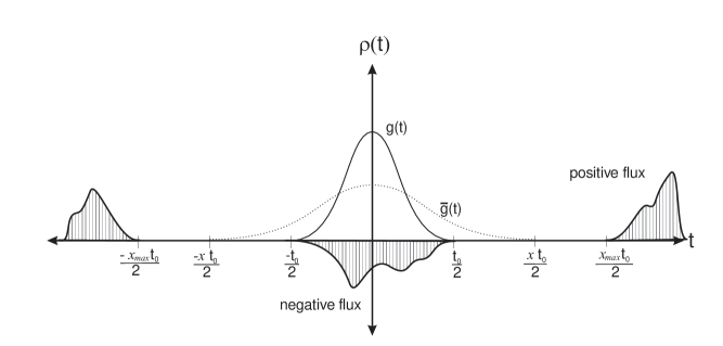
Figure 2: We sample a local distribution of negative energy with a function $g(t)$ and with a scaled version of $g(t)$, namely $\bar{g}(t)=g(t/x)/x$. The quantum inequalities then tell us that there is a maximum scale factor $x_{max}$ beyond which positive energy must be sampled by $\bar{g}(t)$.

To answer these questions we sample the distribution again with a second function $\bar{g}(t)$ that is merely a copy of $g(t)$ scaled by a factor $x\geq 1$:

$$\bar{g}(t)=\frac{1}{x}g\left(\frac{t}{x}\right).$$ (10)

The support of $\bar{g}(t)$ is thus $[-xt_{0}/2,xt_{0}/2]$, and the leading factor of $1/x$ is a normalization constant to give $\bar{g}$ unit integral. If we calculate the minimum negative energy density $\langle\bar{\rho}_{min}\rangle$ allowed by the quantum inequalities using $\bar{g}$ in (4) or (5) for 2D and (6) in 4D Minkowski spacetime we obtain the key result:

$$\langle\bar{\rho}_{min}\rangle=\frac{\langle\rho_{min}\rangle}{x^{d}}.$$ (11)

Here $\langle\rho_{min}\rangle$ is the lower bound associated with $g(t)$ and $d$ is the spacetime dimension (2 or 4). This expression immediately suggests the principle of quantum interest. We have total negative energy $E_{m}=\int_{-t_{0}/2}^{t_{0}/2}\rho(t)dt$ and an average energy density of $\rho_{avg}=E_{m}/t_{0}\approx\langle\rho\rangle$. If we now increase our sampling range to $xt_{0}$, and $\rho(t)$ is zero outside of $[-t_{0}/2,t_{0}/2]$, then $\rho_{avg}$ will scale as $1/x$. But the maximum allowed negative energy density scales as $1/x^{d}$, thus positive energy (and probably quite a lot of it) is eventually needed to satisfy the quantum inequalities.

We can make the preceding statement more precise. Define a constant $y$, with $0<y\leq 1$, such that

$$\langle\rho\rangle=\int_{-t_{0}/2}^{t_{0}/2}g(t)\rho(t)dt=y\langle\rho_{min}\rangle.$$ (12)

Note that for most sampling functions $g(t)$ there will probably not be any quantum state that achieves the minimum ($y=1$). Now stretch $g(t)$ by the factor $x>1$, and to answer the first question we will show that there is a largest possible $x=x_{max}$ allowed by the QI’s if we assume zero energy density outside of the negative pulse, as illustrated in Figure 2:

$$\int_{-xt_{0}/2}^{xt_{0}/2}\rho(t)\bar{g}(t)dt=\frac{1}{x}\int_{-t_{0}/2}^{t_{0}/2}\rho(t)g(t/x)dt\geq\langle\bar{\rho}_{min}\rangle=\frac{\langle\rho_{min}\rangle}{x^{d}}.$$ (13)

Using (12) we can rewrite the inequality as

$$x^{d-1}\leq\frac{1}{y}\frac{\int_{-t_{0}/2}^{t_{0}/2}\rho(t)g(t)dt}{\int_{-t_{0}/2}^{t_{0}/2}\rho(t)g(t/x)dt}.$$ (14)

This clearly shows that if we have some negative energy ($y\neq 0$) then there is an upper bound on $x$, for, recalling that $g(t)$ is positive with a single peak at $t=0$ so that $g(0)\geq g(t/x)\geq g(t)$, one can see that the ratio of the two integrals in (14) is $\leq 1$ (but is at least as large as $\frac{\int_{-t_{0}/2}^{t_{0}/2}\rho(t)g(t)dt}{g(0)\int_{-t_{0}/2}^{t_{0}/2}\rho(t)dt}$). Thus we can write

$$x_{max}^{d-1}=\frac{1}{y}\frac{\int_{-t_{0}/2}^{t_{0}/2}\rho(t)g(t)dt}{\int_{-t_{0}/2}^{t_{0}/2}\rho(t)g(t/x_{max})dt}.$$ (15)

This upper bound depends on the sampling function and in general will over-estimate the maximum allowed separation since a real distribution of energy must satisfy (15) for all choices of $g(t)$.

Without a specific sampling function or energy distribution we cannot reduce (15) any further, but we can see that the range of possible $x$ is most strongly influenced by $y$. If $y=1$ (we have a state that actually achieves the minimum allowed by $g(t)$) then the only way (14) or (15) can be satisfied is if $x=1$; i.e. positive energy must immediately follow and or precede the negative energy. If $y$ is close to zero then $x$ can be large and we can approximate the integral in the denominator of (15) by evaluating $g(t/x)$ at $t=0$:

$$x_{max}^{d-1}\approx\frac{1}{y}\frac{\langle\rho\rangle}{g(0)E_{m}},\ \ \ 1/y\gg 1.$$ (16)

In most situations $\langle\rho\rangle/g(0)E_{m}$ will be a number of order unity. If we have a delta function pulse of negative energy centered at $t=0$ (as considered by Ford and Roman) we obtain a similar relation

$$x_{max}^{d-1}=\frac{1}{y}.$$ (17)

The above expressions (15) - (17) all show that stronger distributions of negative energy (larger y) are required to be close to positive energy (smaller $x_{max}$). Also note that the bound on $x$ is stronger in 4 dimensional spacetime.

To answer the second question, namely whether the quantum interest $\epsilon$ defined by

$$\frac{E_{p}}{|E_{m}|}=(1+\epsilon)$$ (18)

is positive, consider the situation in Figure 3 (note that in this figure we have omitted the $1/x$ normalization constants in the plots of $\bar{g}$), where $E_{p}$ is the total positive energy, i.e. $E_{p}=\int_{t_{1}}^{xt_{0}/2}\rho(t)dt$. Here we stretch $g(t)$ by a new factor $x$ (possibly larger than $x_{max}$, which is the maximum $x$ if we only sample negative energy), and the positive energy flux arrives at time $t_{1}$, with $t_{0}/2\leq t_{1}\leq x_{max}t_{0}/2$. For simplicity we only consider positive energy that arrives after the negative energy, but this doesn’t affect the generality of the argument. Applying the QI’s and scaling relation to this situation yields

$$\int_{-xt_{0}/2}^{xt_{0}/2}\rho(t)\bar{g}(t)dt=\frac{1}{x}\int_{-t_{0}/2}^{t_{0}/2}\rho(t)g(t/x)dt+\frac{1}{x}\int_{t_{1}}^{xt_{0}/2}\rho(t)g(t/x)dt\geq\langle\bar{\rho}_{min}\rangle=\frac{\langle\rho_{min}\rangle}{x^{d}}$$ (19)

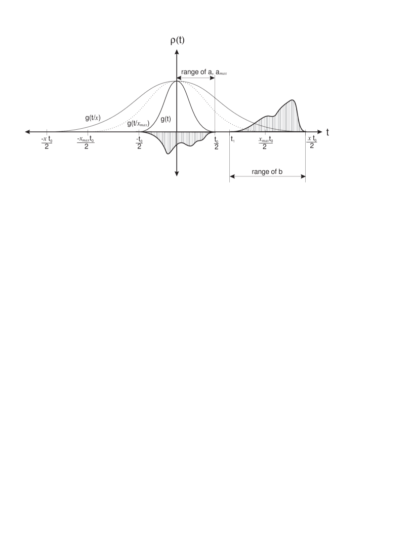
Figure 3: In this situation the positive flux arrives a time $\Delta t=t_{1}-t_{0}/2$ after the negative pulse, and lasts for a time $xt_{0}/2-t_{1}$. The quantum inequalities tell us that the total amount of positive energy must always be larger than the total amount of negative energy.

To simplify the appearance of this expression we assume that $\rho(t)$ is negative semi-definite in the range $[-t_{0}/2,t_{0}/2]$, and positive semi- definite elsewhere (again this does not qualitatively affect the conclusions). Then we can find a number $a$, where $0\leq a<t_{0}/2$, such that $\int_{-t_{0}/2}^{t_{0}/2}\rho(t)g(t/x)dt=g(a/x)E_{m}$, and a number $b$, where $a<t_{1}\leq b<xt_{0}/2$, such that $\int_{t_{1}}^{xt_{0}/2}\rho(t)g(t/x)dt=g(b/x)E_{p}$ (see Figure 3). Thus we can rewrite (19) as

$$-|E_{m}|g(a/x)+E_{p}g(b/x)\geq-\frac{|\langle\rho_{min}\rangle|}{x^{d-1}}.$$ (20)

(This expression is already quite suggestive: if the right hand side of (20) is close to zero then $E_{p}$ will have to outweigh $|E_{m}|$ by roughly $g(a/x)/g(b/x)$ to satisfy the inequality). Using (12) and (15), we can write (20) as

$$-|E_{m}|g(a/x)+E_{p}g(b/x)\geq\left(\frac{x_{max}}{x}\right)^{d-1}\int_{-t_{0}/2}^{t_{0}/2}g(t/x_{max})\rho(t)dt.$$ (21)

As we did for (19), we can simplify (21) using $\int_{-t_{0}/2}^{t_{0}/2}g(t/x_{max})\rho(t)dt=-g(a_{max}/x_{max})|E_{m}|$, where $0\leq a_{max}<t_{0}/2$ (note that $a_{max}$ simply labels the evaluation of the integral when $x=x_{max}$ and doesn’t refer to any maximization of the label $a$ defined earlier; in particular, because $g(t)$ decreases monotonically away from $t=0$, $x<x_{max}$ implies that $a>a_{max}$ and hence $g(a/x)<g(a_{max}/x_{max})$, and vice -versa). This gives, after some rearrangement and utilizing (18)

$$(1+\epsilon)\geq\frac{1}{g(b/x)}\left(g(a/x)-g(a_{max}/x_{max})\left(\frac{x_{max}}{x}\right)^{d-1}\right).$$ (22)

Inequality (22) must be satisfied for all choices of the scaling factor $x$. For smaller $x$ ($x\lesssim x_{max}$) $\epsilon$ can be negative, but we want to show that as $x$ increases eventually $\epsilon$ must become positive. Later we will choose a more restrictive distribution of positive energy to better illustrate quantum interest, but first we will show that (at least when $d=4$) the total amount of positive energy is strictly greater than the total negative energy that passes the observer. To do so, evaluate (22) in the limit as $x\rightarrow\infty$. In this limit for $t=a/x$ and $t=b/x$ we can accurately evaluate $g(t)$ in a Taylor series about $t=0$:

$$g(t)=g(0)-\frac{|g^{\prime\prime}(0)|}{2}t^{2}+O(t^{4}).$$ (23)

There are no odd powers because of the assumed symmetry in $g$, but even if we don’t require $g$ to be symmetric there will not be any $t$ term in the series because of the peak at $t=0$ (which also forces $g^{\prime\prime}(0)$ to be negative). Thus (22) can be written as

$$\epsilon\geq\frac{|g^{\prime\prime}(0)|}{2g(0)}\frac{b^{2}-a^{2}}{x^{2}}-\frac{g(a_{max}/x_{max})}{g(0)}\left(\frac{x_{max}}{x}\right)^{d-1}+O(1/x^{3}).$$ (24)

In the limit $x\rightarrow\infty$, $\epsilon\rightarrow 0$ and when the dimension $d=4$, $\epsilon$ is strictly greater than $0$ for $x$ sufficiently large. In 2 dimensional Minkowski space we can only conclude that $\epsilon$ is at least zero for arbitrary fluxes using the large $x$ behavior of the inequality (22).

To gain more insight into inequality (22) it is useful to restrict the positive flux to last for a time $t_{0}$. Then

$$\frac{xt_{0}}{2}=t_{1}+t_{0}$$ (25)

and

$$\frac{t_{0}}{2}\leq t_{1}\leq\frac{x_{max}t_{0}}{2},$$ (26)

hence

$$3\leq x\leq x_{max}+2.$$ (27)

To obtain a lower bound estimate $\epsilon_{\ell}$ for the quantum interest $\epsilon$, set $a=t_{0}/2$, $a_{max}=0$ and $b=t_{1}$ in (22) (this will be a good approximation for larger $x$; see Figure 3)

$$1+\epsilon_{\ell}\geq\frac{g(t_{0}/2x)-g(0)(x_{max}/x)^{d-1}}{g((t_{0}/2)(1-2/x))},$$ (28)

where we have used (25) to eliminate $t_{1}$ from the expression. For a concrete example we will use the polynomial sampling function with n=2 (9), i.e. $g(t)\propto(t^{2}-t_{0}^{2}/4)^{2}$. Define $z\equiv\frac{\Delta t}{t_{0}}=\frac{t_{1}-t_{0}/2}{t_{0}}$, so $z$ is the time interval separating the positive and negative pulses divided by $t_{0}$.Using (25) to (27) we can find the range of $z$: $0\leq z\leq z_{max}$, $z_{max}=(x_{max}-1)/2$. When $x=x_{max}$ (and the exact inequality (22) gives $\epsilon\geq-1$), $z=z_{max}-1$. With these definitions (28) becomes (after some simplification)

$$1+\epsilon_{\ell}\geq\frac{1}{4}\left[(z+2)^{2}-\frac{(z+3/2)^{5-d}(z_{max}+1/2)^{d-1}}{(z+1)^{2}}\right].$$ (29)

For large $z$ and $z_{max}$

$$\epsilon_{\ell}\gtrsim z(\frac{z}{4}+1)-\frac{z^{3-d}z_{max}^{d-1}}{4}\left(\frac{3(5-d)-4}{2z}+\frac{d-1}{2z_{max}}+1\right).$$ (30)

When $z$ is in the range $[z_{max}-1,z_{max}]$, (30) is almost a straight line, with $\epsilon_{\ell}$ ranging from a minimum of $-5/4$ to a maximum of $z_{max}/4$ in 2D spacetime (compare Figure 4 where expression (29) is plotted), and from $-9/8$ to $(3/4)z_{max}$ in 4D spacetime (compare Figure 5). This shows quite clearly that quantum interest grows (almost linearly) as the pulse separation increases. But a note of caution: this example will give an accurate lower bound on the quantum interest only if our choice of sampling function doesn’t overestimate the “real” $x_{max}$ or $z_{max}$ for a given distribution of negative energy. Recall that the “real” $x_{max}$ must satisfy inequality (15) for any choice of sampling function. For example, a sharply peaked sampling function (e.g. (9) with large $n$) will not give very stringent lower bounds on $\langle\rho_{min}\rangle$, and consequently (15) will overestimate $x_{max}$ for a small pulse of negative energy ($y\ll 1$). A similar analysis to that above would then seem to indicate that the quantum interest diverges in the limit as $n\rightarrow\infty$ at $z=z_{max}$, but in truth the value of $z_{max}$ was overestimated.

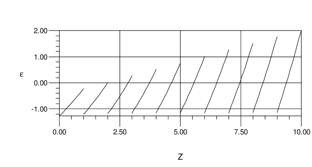
Figure 4: A lower bound estimate (29) for the quantum interest $\epsilon$ as a function of pulse separation $z=\Delta t/t_{0}$ in 2D Minkowski spacetime. Ten curves are plotted for values of $z_{max}$ from 1 to 10; the range of each curve is $[z_{max}-1,z_{max}]$. The larger $z_{max}$ the less negative energy was sampled, allowing greater separation of the fluxes. The estimate (29) is closer to the true lower bound for larger $z$. The width of the positive pulse in this example is $t_{0}$, and the sampling function (9) with $n=2$ was used.

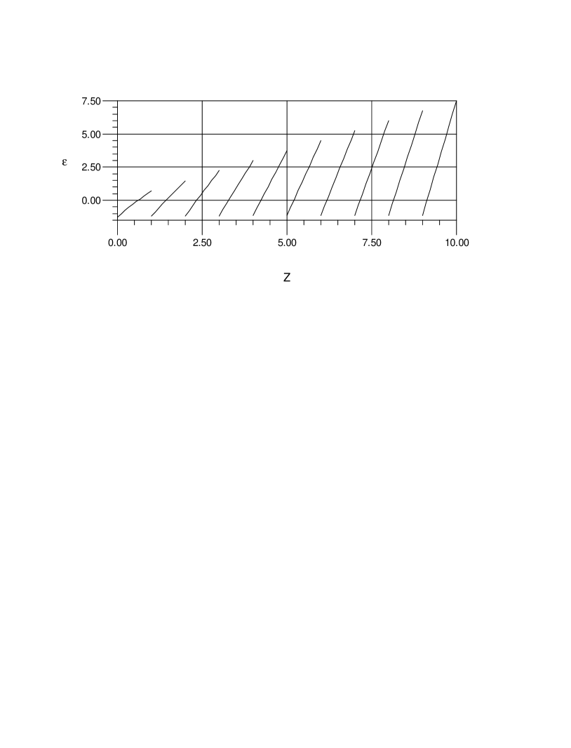
Figure 5: The same information as shown in Figure (4) but in 4D Minkowski spacetime.

4 Massive scalar fields

In this section we will briefly show that the quantum interest inequalities (14) and (22) and hence all the results from the previous section also apply to the massive scalar field in 4 dimensional Minkowski spacetime.

Fewster and Eveson [14] obtained the following expression for $\langle\rho_{min}\rangle$ in $4D$ Minkowski spacetime for a scalar field of mass $m$:

$$\langle\rho_{min}\rangle=-A\int_{0}^{\infty}ds\int_{m}^{\infty}d\omega_{k}\ \omega_{k}^{2}[\omega_{k}^{2}-m^{2}]^{1/2}|\widehat{g^{1/2}}(s+\omega_{k})|^{2},$$ (31)

where $A$ is a positive constant, $\widehat{g^{1/2}}(s)$ is the Fourier transform of $g^{1/2}(t)$, and one integrates over the spectrum of field modes (i.e. $\omega_{k}=\sqrt{|k|^{2}+m^{2}}$, $\vec{k}$ is the 3-momentum of a mode with frequency $\omega_{k}$).

If $\langle\rho_{min}\rangle(m)$ denotes the minimum negative energy bound for a field of mass $m$ with sampling function $g(t)$, then

$$\langle\bar{\rho}_{min}\rangle(m)=\frac{\langle\rho_{min}\rangle(mx)}{x^{4}},$$ (32)

where $\langle\bar{\rho}_{min}\rangle(m)$ is the minimum bound with a sampling function $\bar{g}(t)=g(t/x)/x$ (the Fourier transform of the scaling relation is $\widehat{\bar{g}^{1/2}}(s)=\sqrt{x}\widehat{g^{1/2}}(sx)$). But notice from (31) that $\langle\rho_{min}\rangle(mx)\geq\langle\rho_{min}\rangle(m)$ for $x\geq 1$ (due to the $m$ dependance in the integrand and lower limit of the second integral), hence

$$\langle\bar{\rho}_{min}\rangle(m)\geq\frac{\langle\rho_{min}\rangle(m)}{x^{4}}.$$ (33)

Thus a massive scalar field will have tighter constraints on allowed negative energies than a massless field (compare (11)), and all the inequalities derived in the previous section remain valid for a massive field. (In 2D Minkowski space (32) holds with $x^{4}$ replaced by $x^{2}$, but one cannot conclude that (33) is valid $\forall x$.)

5 Beyond scalar fields in Minkowski spacetime

The scaling argument used to prove quantum interest for scalar fields might readily be applied to other quantum fields, such as the Electromagnetic (EM) field or Dirac field, and possibly to certain curved spacetimes or Minkowski space with boundary conditions as in the Casimir effect.

Ford and Roman found a quantum inequality for EM fields in 4D Minkowski space using a Lorentzian sampling function [15]:

$$\langle\rho\rangle_{EM}\geq-\frac{3}{16\pi^{2}t_{0}^{4}}.$$ (34)

This expression certainly indicates that a scaling relation like (11) holds for EM fields. The only complication to obtaining definitive results in this case is that the Lorentzian sampling function does not have compact support, so one cannot rule out the possibility that long distance interference effects may spoil quantum interest for arbitrary energy fluxes of the EM field (though this seems unlikely).

There is some evidence that the Dirac field might also satisfy negative energy inequalities similar to those of scalar and EM fields. Vollick has recently shown that a superposition of two single particle electron states can exhibit negative energy densities, but they are constrained by an inequality identical in form to that of the EM and scalar fields [16].

Fewster and Teo [17] have derived lower bounds of the form (31) for states of scalar quantum fields in static, curved spacetimes (those with timelike killing vector fields that are hypersurface orthogonal). The scaling argument will work in certain static spacetimes. For example one can easily show that the scaling relation (33) holds in an open static Robertson-Walker universe ($ds^{2}=-dt^{2}+a^{2}[d\xi^{2}+sinh^{2}(\xi)d\Omega^{2}]$, $a$ is consant), as the lower bound for the sampled energy density takes the form [17]:

$$\langle\rho_{min}\rangle=-A\int_{0}^{\infty}ds\int_{C}^{\infty}d\omega_{k}\ \omega_{k}^{2}[\omega_{k}^{2}-C^{2}]^{1/2}|\widehat{g^{1/2}}(s+\omega_{k})|^{2},$$ (35)

where $C=\sqrt{1/a^{2}+m^{2}}$ and $m$ is the mass of the scalar field (compare (31)).

In a spacetime with a non-zero expectation value $\rho_{0}$ for the ground state energy density, such as the Boulware state outside a static star or with the Casimir effect between two conducting plates, one might expect a scaling relation of the form

$$\langle\bar{\rho}_{min}\rangle=\frac{\langle\rho_{min}\rangle}{x^{d}}+\rho_{0}$$ (36)

to hold. In other words, perhaps one may be able prove the quantum interest conjecture for energies relative to the ground state energy – see [9] for examples where the quantum inequalities take on the from $\langle\rho\rangle\geq$ free field term + Casimir terms.

6 Conclusion

In this paper we have proven the quantum interest conjecture of Ford and Roman for arbitrary distributions of negative energy of scalar fields in 4D Minkowski spacetime (slightly weaker results hold in 2D). Specifically, any flux of negative energy flowing past an inertial observer must be followed or preceded by positive energy within a finite time interval that decreases the larger the amount of negative energy. In addition, the total amount of positive energy seen ($E_{p}$) is always greater than the total amount of negative energy ($-|E_{m}|$). In a more restricted scenario where the duration of the positive and negative fluxes are equal, we showed that the quantum interest $\epsilon\equiv\left(\frac{E_{p}}{-|E_{m}|}-1\right)$ grew almost linearly with pulse separation.

The nature of existing QI’s for EM fields, the Dirac field and scalar fields in certain static spacetimes suggests that quantum interest may have broader application than free scalar fields in Minkowski spacetime. In a situation where the ground state energy density of the field is non- zero (e.g. in the Casimir effect) we may still expect quantum interest to hold, but then “negative” energy would refer to energies less than that of the ground state.

An important consequence of quantum interest is what it tells us about the nature of negative energies in free fields. A local pulse of negative energy is not an entity that can be manipulated or interacted with independently of the accompanying positive energy that must be near by. Even if there are states where the positive and negative energies are separated by a sizeable distance (as suggested by (14) when the amount of negative energy is very small), one could still only interact with the pulse pair as a single entity. For example, absorbing, reflecting or scattering only the positive part of the flux would create an isolated negative pulse, violating the quantum inequalities. Furthermore, this implies that one cannot subject a hot body to a net flux of negative energy that otherwise might have lowered its entropy in violation of the $2^{nd}$ law of thermodynamics.

Acknowledgement

I would like to thank Werner Israel for many stimulating discussions.

References

- [1] H. Epstein, V. Glaser, and A. Jaffe, Nuovo Cim. 36, 1016 (1965).
- [2] M. Morris and K. Thorne, Am. J. Phys. 56, 395 (1988).
-
[3]
M. Alcubierre, Class. Quantum Grav. 11, L73
(1994),
S.V. Krasnikov, Phys. Rev. D 57, 4760 (1998). - [4] M. Morris, K. Thorne, and U. Yurtsever, Phys. Rev. Lett. 61, 1446 (1988).
- [5] L.H. Ford, Proc. Roy. Soc. Lond. A 364, 227 (1978).
- [6] P.C.W. Davies, Phys. Lett. 113B, 215 (1982).
- [7] L.H. Ford, Phys. Rev. D 43, 3972 (1991).
- [8] L. H. Ford and T. A. Roman, Phys. Rev. D51, 4277 (1995).
- [9] for references see M.J. Pfenning and L. H. Ford, Quantum Inequality Restrictions on Negative Energy Densities in Curved Spacetimes, gr-qc/9805037
- [10] M.J. Pfenning and L.H. Ford, Class. Quantum Grav. 14, 1743 (1997)
- [11] L.H. Ford and T.A. Roman, Phys. Rev. D 53, 5496 (1996)
- [12] L.H. Ford and T.A. Roman, The Quantum Interest Conjecture, gr-qc/9901074
- [13] É. É. Flanagan, Phys. Rev. D 56, 4922 (1997), gr-qc/9706006.
- [14] C.J. Fewster and S.P. Eveson, Phys. Rev. D 58, 084010 (1998), gr-qc/9805024.
- [15] L. H. Ford and T. A. Roman, Phys. Rev. D 55, 2082 (1997), gr-qc/9607003.
- [16] D. N. Vollick, Phys. Rev. D 57, 3483 (1998).
- [17] C.J. Fewster and E. Teo, Bounds on negative energy densities in static space-times, gr-qc/9812032.
-
[18]
L. H. Ford and T. A. Roman, Phys. Rev. D
51, 4277 (1995).
U. Yurtsever, Phys. Rev, D 51, 5797 (1995)
M. J. Pfenning and L. H. Ford, Phys. Rev. D 55, 4813 (1997)
M. J. Pfenning and L. H. Ford, Phys. Rev. D 57, 3489 (1998).