Thick Domain Wall Universes

Abstract

We investigate the spacetime of a thick gravitating domain wall for a general potential $V(\Phi)$. Using general analytical arguments we show that all nontrivial solutions fall into two categories: those interpretable as an isolated domain wall with a cosmological event horizon, and those which are pure false vacuum de Sitter solutions. Although this latter solution is always unstable to the field rolling coherently to its true vacuum, we show that there is an additional instability to wall formation if the scalar field does not couple too strongly to gravity. Using the $\lambda\Phi^{4}$ and sine-Gordon models as illustrative examples, we investigate the phase space of the gravitating domain wall in detail numerically, following the solutions from weak to strong gravity. We find excellent agreement with the analytic work. Then, we analyse the domain wall in the presence of a cosmological constant finding again the two kinds of solutions, wall and de Sitter, even in the presence of a negative cosmological constant.

I Introduction

The study of topological defects has wide applicability in many areas of physics. In the cosmological arena, defects have been put forward as a possible mechanism for structure formation [1], and while recent work on global defects [2, 3] indicates that these were probably not responsible for structure formation, the intriguing discovery of a non-gaussian signature in the microwave background [4] leaves open the possibility that defects were around at some point in the evolution of the universe.

Of all the topological defects, domain walls are the most deceptively simple to study. They correspond to solitons in 1+1-dimensions, which are extended in two spatial directions to form a wall structure. Because they depend on only one spatial coordinate, the distance from the wall, the solutions in the absence of gravity can often be written in closed analytic form, and for certain potentials the models are completely integrable and the defects have the full interpretation of solitary travelling waves. In the presence of gravity however, the situation changes, gravity destroys the integrability of the theory, and also, except in a perturbative sense, the analytic nature of the solutions. Fortunately, since the walls correspond approximately to hypersurfaces in spacetime, there is a well defined way of analysing their gravity using Israel’s thin wall formalism [5], in which the wall is approximated by an infinitesimally thin hypersurface, and most of the literature concerning domain wall gravity uses this method.

The domain wall is a rather interesting object gravitationally: unlike almost all of the other topological defects (the exception being the global string [6]), its metric is not static but time-dependent [7, 8], having a de Sitter-like expansion in the plane of the wall. Observers experience a repulsion from the domain wall, and there is an horizon at finite proper distance from the defect’s core. This horizon can be interpreted as a facet of the choice of coordinates, which usually use the flat space wall solution as a starting point, and impose planar symmetry on the domain wall spacetime. However, it is possible to use a different set of coordinates [8, 9] in which the wall has the appearance of a bubble which contracts in from infinite radius to some minimum radius, then re-expands, undergoing uniform acceleration from the origin. The ‘horizon’ is then simply the lightcone of the origin in these coordinates, and is somewhat similar to the horizon of Rindler spacetime.

The crucial physical difference of a domain wall spacetime, as opposed to that of the local cosmic string or monopole, is the presence of this cosmological horizon, which introduces a second length scale into the system. Ordinarily, a defect possesses one length scale, $w$, which is a measure of its thickness. However, the distance to the event horizon of the domain wall gives another length scale, $z_{\rm h}$, which can be compared to $w$. Since these lengths are given in terms of the coupling constants of the theory, taking a thin wall limit turns out to be a very artificial construction in terms of these underlying parameters, and the issue of the self-gravity of thick walls becomes more pertinent. After the original work by Vilenkin, Ipser and Sikivie [7, 8], attempts focussed on trying to find a perturbative expansion in the wall thickness [10, 11] both for the purpose of discovering the motion of the wall, as well as verifying that the hypersurface formalism was a good approximation to the true gravitational field. These results backed up the thin wall approximation, the main difference being the presence of a sub-dominant tension transverse to the wall.

With the suggestion of Hill, Schramm and Fry [12] of a late time phase transition with thick domain walls, there was some effort at finding exact thick solutions [13, 14], see also [15, 16]. However, such defects were supposed to be thick by virtue of the low temperature of the phase transition responsible for defect formation. The suggestion that Planck scale topological defects could be responsible for inflation [17, 18] then reopened the issue of thick domain walls. ‘Thick’ then means thick compared to their natural de Sitter horizon, and therefore this appears to be a very strong gravity situation. The issue of whether a domain wall can survive in a Friedmann-Robertson-Walker (FRW) universe with horizon size comparable to wall thickness has been analysed in some detail for the case of no gravitational back reaction of the wall on the FRW background [19, 20], and in the case of Euclidean instantons on a de Sitter background including self-gravity [21, 22]; however, to our knowledge, a systematic analysis of the strong self-gravity of thick domain walls with an arbitrary field theory potential has not been carried out.

In this paper we perform a detailed analysis of the strong gravity of thick domain walls. With a combination of analytical and numerical results, we map out the parameter space in which a wall-like solution exists. Although we focus on two main examples of the sine-Gordon and $\lambda\Phi^{4}$ wall, we also illustrate to what extent, and for what potentials, the results will also hold in general. We begin in the next section by setting out the general formalism for a thick domain wall, deriving the metric and Einstein equations, as well as defining what we mean by a ‘wall’ solution. We also show how to generalise a coordinate transformation which takes a planar domain wall spacetime with an horizon into a flat spacetime with an accelerating wall to the case of walls with finite thickness. The solution outside the wall horizon is shown to be related to an FRW cosmology with a slowly rolling scalar field.

In the following section we derive analytic results for the thick wall. It turns out that there are two possibilities for the scalar field from which the ‘wall’ is constituted: it can either be a planar wall or a de Sitter solution. Since the de Sitter solution is always possible, but not necessarily stable, we derive analytic bounds on the gravitational coupling strength of the wall for when the de Sitter solution is the only possible solution, and when it becomes unstable to decay into a wall-like solution. Note that the de Sitter solution always contains an instability to the field rolling coherently down the potential well — we will not be interested in these instabilities, only in those which would lead to the formation of a domain wall. We derive these bounds for both our chosen field theory models, as well as for a general potential. We then provide, in the case of weak gravitational coupling, some perturbative solutions for the wall and its gravitational fields. These can be readily compared to existing results in the literature. We then present numerical results backing up and extending the analytic work. In the penultimate section we consider the domain wall in the presence of a cosmological constant, and conclude in the final section.

II Plane-symmetric spacetimes

We start by setting up the general framework for a domain wall coupled to gravity. We initially consider a general matter Lagrangian

$${\cal L}_{\mbox{M}}=(\nabla_{a}\Phi)^{2}-U\left(\Phi\right),$$ (1)

where $\Phi$ is a real Higgs field and the symmetry breaking potential $U(\Phi)$, has a discrete set of degenerate minima. We assume that the spacing of these minima is proportional to the (dimensionful) parameter $\eta$, which sets the symmetry breaking scale, and that $U(\Phi)$ is characterised by a scale $V_{\mbox{F}}=U(\Phi_{\mbox{F}})$, where $\Phi_{\mbox{F}}$ is a local false vacuum situated between successive minima ($\Phi_{\mbox{F}}=0$ is a conventional choice). For example, in the usual ‘kink’ model, $U(\Phi)=\lambda\left(\Phi^{2}-\eta^{2}\right)^{2}$, and we see $\eta$ directly, with $V_{\mbox{F}}=\lambda\eta^{4}$. For convenience, we scale out dimensionful parameters via

$$X=\Phi/\eta,\qquad\epsilon=8\pi G\eta^{2}.$$ (2)

The dimensionless parameter $\epsilon$, which we call gravitational strength parameter, characterises the gravitational interaction of the Higgs field. Then, defining $V(X)=U(\eta X)/V_{\mbox{F}}$,

$$8\pi G{\cal L}_{\mbox{M}}={\epsilon\over w^{2}}\left[w^{2}(\nabla_{a}X)^{2}-V(X)\right],$$ (3)

where $w=\sqrt{\epsilon\over 8\pi GV_{\mbox{F}}}$ represents the inverse mass of the scalar after symmetry breaking, and of course will also characterise the width of the wall defect within the theory. The equations of motion following from (3) are simply

$$\Box X+{1\over 2w^{2}}{\partial V\over\partial X}=0.$$ (4)

Without loss of generality we can set $w=1$ (which amounts to choosing ‘wall’ units rather than Planck units) and, looking for a static solution in flat space, we see that (4) can be integrated directly to give

$$X^{\prime 2}=V(X),$$ (5)

which has an implicit solution

$$\int^{X}_{X_{\mbox{F}}}{dX\over\sqrt{V(X)}}=z-z_{0},$$ (6)

where $X_{\mbox{F}}=X(z_{0})$ is the false vacuum. For example, in the $\lambda\Phi^{4}$ model above, $z-z_{0}=\int_{0}^{X}dX/(1-X^{2})=\tanh^{-1}X$, and we get the usual kink solution centered on $z_{0}$: $X=\tanh(z-z_{0})$. Another model that we will be exploring in detail is the sine-Gordon model, with $V(\Phi)=V_{\mbox{F}}[1+\cos(\Phi/\eta)]/2$, in which case $z-z_{0}=2\ln\tan(\pi/4+X/4)$.

We now look for a plane-symmetric gravitating domain wall solution, since this represents the most obvious intuitive generalization of the flat space domain wall. We will consider coordinate transformations of this solution at the end of the section. The metric therefore will have planar symmetry (i.e. Killing vectors $\partial_{x},\partial_{y},x\partial_{y}-y\partial_{x}$), and in addition will display reflection symmetry around a surface, $z=0$ say, which represents the location of the wall (defined by $X=X_{\rm F}$). If we choose $z$ to be the proper distance from the wall, then the metric may be written as

$$ds^{2}=A^{2}(z)dt^{2}-B^{2}(z,t)\left(dx^{2}+dy^{2}\right)-dz^{2},$$ (7)

with the associated Einstein equations derived from the Lagrangian (1) coupled to gravity through the usual Hilbert term, ${\cal L}_{\mbox{G}}=-R/2\epsilon$, being

$$R_{ab}=2\epsilon X_{,a}X_{,b}-\epsilon\,V(X)\,g_{ab}.$$ (8)

Before writing these equations explicitly, we will first examine what we mean by a domain wall solution, since this will require some rather specific boundary conditions at $z=0$, and for large $z$. We will define a wall solution to be a function $X(z)$ of the proper distance from the wall which at $z=0$ is at a local maximum of $V(X)$, $X_{\mbox{F}}$, and which falls towards distinct minima on either side of the wall. Assuming that $V(X)$ is locally symmetric around the maximum, then $(X(z)-X_{\rm F})$ will be an odd function of $z$. This restriction embodies the idea of a defect, in which the field falls to distinct vacua on either side of its core, and settles to a topological, rather than radiative, configuration. It is possible that the only nonsingular solution satisfying these criteria is $X\equiv X_{\mbox{F}}$, in which case the spacetime will be de Sitter; indeed, this is always a possible solution to the equations of motion satisfying the above criteria, though it will not necessarily be stable. Clearly, there is always an instability corresponding to a coherent roll of the field towards one of its vacuum values, however, since we are interested in spacetimes with the interpretation of a domain wall, we will ignore this mode, and say that de Sitter spacetime is ‘stable’ if there is no odd perturbation of $(X-X_{\rm F})$ which is growing in time. As we will see, the scalar field does not fall all the way to its minimum value within the range of validity of the coordinates in (7), which is why we do not place any specific boundary conditions on $X$ for large $z$, however, it will turn out that we require $X^{\prime}(z_{h})=0$ for a nonsingular solution. Finally, we can choose $t$ to set $A(0)=1$, and reflection symmetry requires $A^{\prime}(0)=0$.

Turning to the Einstein equations (8), we see that

$$R_{zt}={{\dot{B}}A^{\prime}\over BA}-{{\dot{B}}^{\prime}\over B}=0$$ (9)

which implies $B=b(t)A(z)$. Then the relation

$$R^{t}_{t}-R^{x}_{x}=A^{2}\left({{\dot{b}}^{2}\over b^{2}}-{{\ddot{b}}\over b}\right)=0$$ (10)

yields

$$b(t)={\rm e}^{kt},$$ (11)

so that the equations of motion for the gravitating wall finally reduce simply to

$$X^{\prime\prime}+3{A^{\prime}\over A}X^{\prime} = {1\over 2}{\partial V\over\partial X}$$ (13)

$${A^{\prime\prime}\over A} = -{\epsilon\over 3}\left[2X^{\prime 2}+V(X)\right]$$ (14)

$$\left({A^{\prime}\over A}\right)^{2} = {k^{2}\over A^{2}}+{\epsilon\over 3}\left[X^{\prime 2}-V(X)\right].$$ (15)

Note that since $A^{\prime\prime}\leq 0$, once $A^{\prime}$ becomes negative it will always be bounded away from zero, therefore there is some finite $z_{\rm h}$ for which $A(z_{\rm h})=0$, and we have either a physical or coordinate singularity. Thus we see immediately that there is no nonsingular solution with $k^{2}=0$. It is also easy to see that the false vacuum de Sitter solution is given by $X=X_{\mbox{F}}$, $A=\cos kz$, $k^{2}=\epsilon/3$.

Determining therefore whether or not a wall solution exists reduces to investigating the system of equations (II). Clearly, for small $\epsilon$ we might expect a wall solution to the above equations to exist, and to be given by a perturbative expansion around flat space. For large $\epsilon$, since $A^{\prime}=O(\epsilon)$, the $A^{\prime}X^{\prime}/A$ term in (13) will drive the solution to a singularity for nonzero $(X-X_{\mbox{F}})$, hence for large $\epsilon$ we expect only the de Sitter solution. For intermediate values of $\epsilon$, except for some very special cases, an analytic solution does not exist and we have to numerically integrate the equations.

Before proceeding with the details of this analysis, we conclude this section by commenting on a coordinate transformation of the plane symmetric metric (7), which transforms the defect into an accelerating bubble wall. Defining

$$x^{*} = A(z){\rm e}^{kt}x$$ (17)

$$y^{*} = A(z){\rm e}^{kt}y$$ (18)

$$t^{*}-z^{*} = -{1\over k}A(z){\rm e}^{kt}$$ (19)

$$t^{*}+z^{*} = \phantom{-}{1\over k}A(z){\rm e}^{-kt}-k(x^{2}+y^{2})A(z){\rm e}^{kt}$$ (20)

gives an alternate form of the line element:

$$ds^{2}=dt^{*2}-dx^{*2}-dy^{*2}-dz^{*2}+\left({A^{\prime 2}\over k^{2}}-1\right)dz^{2},$$ (21)

where $z$ is given implicitly by

$$k^{2}(t^{*2}-{\bf x}^{*2})=-A^{2}(z).$$ (22)

The wall (i.e. the zero of $X-X_{\rm F}$) is located at ${\bf x}^{*2}-t^{*2}=1/k^{2}$, and as we will see, for small values of the gravitational coupling $\epsilon$, $A^{\prime}$ rapidly approaches $k=O(\epsilon)$ outside the core of the wall. Therefore, we see that the spacetime in these coordinates is approximately flat, with the wall being located at a spacelike hyperboloid at a distance $1/k$ from the origin. This corresponds to a wall undergoing uniform acceleration, contracting in from infinity, reaching a minimum radius, and re-expanding outwards. The horizon ($A(z_{\rm h})=0$ in the old coordinates) is now the lightcone centered on the origin, and the region exterior to the horizon is the causal future and past of the origin. Thus the coordinate transformation (II) generalises the thin wall transformation given in [8], and discussed in detail in section three of [9].

For larger values of $\epsilon$ the spacetime will not be flat, and $X$ will not be at its true vacuum value near the horizon. In particular, setting $t^{*}=\tau\cosh\psi$, $x^{*}=\tau\sinh\psi\sin\theta\cos\phi$, etc., then gives a rather familiar form for the metric exterior to the horizon, i.e. inside the lightcone of the origin:

$$ds^{2}=C^{2}(\tau)d\tau^{2}-\tau^{2}\left[d\psi^{2}+\sinh^{2}\psi(d\theta^{2}+\sin^{2}\theta d\phi^{2})\right],$$ (23)

the metric of an open FRW universe. Thus if the scalar field is not at its vacuum value at the horizon, its evolution outside the horizon is given by the rolling of a scalar towards its minimum in an open FRW model, a well studied problem!

III self-gravitating domain walls

We now want to find solutions to (II) representing an isolated domain wall for various values of the parameter $\epsilon$. We start by considering a general potential, $V(X)$, finding an analytic perturbative solution for small $\epsilon$, and showing that if $\epsilon$ is sufficiently large there is no wall solution. We also demonstrate an instability of the false vacuum de Sitter solution to wall formation for $\epsilon\leq\epsilon_{\rm max}$, where $\epsilon_{\rm max}$ depends on the second derivative of the potential at the origin. We then explore the particular cases of the $\lambda\Phi^{4}$ kink and the sine-Gordon model in some detail, first making reference to the analytic work, then describing the solutions for intermediate values of $\epsilon$ with the help of numerical work. Both analytic and numerical work show the presence of a phase transition in the behaviour of the solutions between wall existence and nonexistence.

It is clear that when the gravitational strength parameter is set to zero, one gets the flat space solution $A=1$, with $X$ being given by (6). Let us now consider small values of $\epsilon$, typically $\epsilon\ll 1$. Then we can expand the fields $X$ and $A$ in powers of $\epsilon$

$$X = X_{0}+\epsilon X_{1}+O\left(\epsilon^{2}\right)$$ (25)

$$A = A_{0}+\epsilon A_{1}+O\left(\epsilon^{2}\right),$$ (26)

where $X_{n}$, $A_{n}$ are now independent of $\epsilon$ and $A_{0},X_{0}$ are the flat space solutions.

The field equations (II) to lowest order in $\epsilon$ give

$$A_{1}^{\prime\prime} = -{1\over 3}\left[2X_{0}^{\prime 2}+V(X_{0})\right]=-X_{0}^{\prime 2}$$ (28)

$$X_{1}^{\prime\prime} = -3A_{1}^{\prime}X_{0}^{\prime}+{1\over 2}X_{1}{\partial^{2}V\over\partial X^{2}}\bigg{|}_{X_{0}(z)}.$$ (29)

The boundary conditions of $A$ and $X$ give

$$A_{1}(0)=A_{1}^{\prime}(0)=0,\qquad X_{1}(0)=0,\qquad X_{1}\to 0\mbox{ for large }z;$$ (30)

(28) and (29) can be integrated to give

$$A_{1}=-\int\!\!\!\!\int V(X_{0})dz=-\int{dX\over\sqrt{V}}\int\sqrt{V}dX$$ (31)

and

$$X_{1}=-{3\over 2}X_{0}^{\prime}\int{dz\over X_{0}^{\prime 2}}\left(A_{1}^{\prime 2}-{k^{2}\over\epsilon^{2}}\right)dz,$$ (32)

which can also be expressed as an implicit integral in terms of $V(X)$ and $X$. Finally, noting that

$$X_{0}^{\prime}X_{1}^{\prime}-X_{1}X_{0}^{\prime\prime}={3\over 2}A_{1}^{\prime 2}+X_{0}^{\prime}(0)X_{1}^{\prime}(0),$$ (33)

(15) implies

$$k^{2}=\epsilon^{2}\left[A_{1}^{\prime 2}+{2\over 3}(X_{1}X_{0}^{\prime\prime}-X_{0}^{\prime}X_{1}^{\prime})\right]=-{2\epsilon^{2}\over 3}X_{0}^{\prime}(0)X_{1}^{\prime}(0).$$ (34)

Before exploring these solutions for specific models for $V(X)$, we can make some general statements about the self-gravitating wall. First of all, since $A_{1}^{\prime\prime}$ is strictly negative, $A$ will asymptote $1-kz$, where $k$ is O($\epsilon$) from the above relation. This means that $A_{1}$ will cease to be small at a distance of order $\epsilon^{-1}$ from the wall, and our expansion procedure strictly speaking breaks down. However, since $A_{1}^{\prime}$ is not growing, it is clear that continuing the expansion to higher orders in $\epsilon$ will merely produce minor corrections to $A$, and will not alter the qualitative behaviour, namely, that $A(z)$ has a zero at a distance of order $\epsilon^{-1}$ from the wall (see figure 2). Since $g_{tt}=A^{2}$ this is simply the event horizon which is familiar from the thin wall approximation.

As $\epsilon$ increases, the effect of the scalar field’s energy-momentum on the geometry increases, and we expect the horizon to move closer to the wall, roughly until $\epsilon={\rm O}(1)$. For large $\epsilon$, the expected horizon would be well inside the core of the wall and two possibilities now emerge. First of all, the scalar field could simply ignore the geometry, and fall away minutely from its false vacuum, causing an horizon at some small value of $z$. Since the spatial gradient of such a solution would be relatively small, the energy-momentum would be vacuum dominated, and we would expect the spacetime to be very close to the de Sitter solution. Outside the horizon, the scalar field would roll to its vacuum value as described in the last section. The alternative is that there is a phase transition in the behaviour of $X$, that is, that $X$ either has some nontrivial odd form, approaching reasonably close to its vacuum value at the horizon, or $X\equiv X_{\mbox{F}}$. In other words, $X$ must either roll significantly away from $X_{\mbox{F}}$, or not at all. There are two reasons why we expect the latter scenario to hold. The first is that Basu and Vilenkin [21] observed just such a phase transition in studying the problem of wall instantons. The other reason for suspecting a phase transition lies in the behaviour of field theory solutions on compact surfaces. For example, two of the authors have studied a cosmic string interacting with the event horizon of an extremal black hole [23]. There, there are nontrivial solutions with the string piercing the horizon while the string fields can fall reasonably close to their vacuum values around the horizon; however, there is a transition when the string becomes sufficiently thick relative to the black hole: the event horizon can no longer support a nontrivial solution and the flux of the string is expelled — the only horizon solution is the trivial one.

First of all, let us show that for small $\epsilon$ the false vacuum de Sitter solution is unstable. Recall that the de Sitter solution is

$$ds^{2}=\cos^{2}(kz)dt^{2}-{\rm e}^{2kt}\cos^{2}(kz)(dx^{2}+dy^{2})-dz^{2}$$ (35)

with $X\equiv X_{\mbox{F}}$ and $k^{2}=\epsilon/3$. This solution will be ‘stable’ (i.e., stable to wall formation) if there is no perturbation of $X-X_{\rm F}$ which is an odd function of $z$ and growing in time. Setting $X=X_{\mbox{F}}+\xi$, and noting that corrections to the geometry are O($\xi^{2}$), we see that an instability must satisfy the time-dependent linearized perturbation equation

$$\xi^{\prime\prime}-3k\tan(kz)\xi^{\prime}-\sec^{2}(kz)[\ddot{\xi}+2k\dot{\xi}]-\frac{1}{2}\xi{\partial^{2}V\over\partial X^{2}}\bigg{|}_{X_{\mbox{F}}}=0$$ (36)

(where a dot indicates differentiation with respect to $t$). This equation does indeed have unstable solutions for $k^{2}=\epsilon/3<|V^{\prime\prime}(X_{\rm F})|/8$, the dominant instability being given by

$$\xi={\rm e}^{k\nu t}\sin kz(\cos kz)^{\nu}$$ (37)

with

$$\nu=-{5\over 2}+{1\over 2}\sqrt{9-2V^{\prime\prime}(X_{\mbox{F}})/k^{2}}.$$ (38)

Thus for $\epsilon$ smaller than

$$\epsilon_{\rm max}=\frac{3}{8}\;\left|V^{\prime\prime}(X_{\mbox{F}})\right|,$$ (39)

the de Sitter solution is unstable to wall formation.

Now let us examine whether a wall solution can exist for large $\epsilon$. For a nontrivial wall solution, we require $X^{\prime}(0)>0$, and for a nonsingular solution, we require $X^{\prime}(z_{\rm h})=0$. Now taking the derivative of the field equation (13) we get

$$X^{\prime\prime\prime}=-3{A^{\prime}\over A}X^{\prime\prime}+X^{\prime}\left[-3{A^{\prime\prime}\over A}+3\left({A^{\prime}\over A}\right)^{2}+\frac{1}{2}{\partial^{2}V\over\partial X^{2}}\right]=-3{A^{\prime}\over A}X^{\prime\prime}+X^{\prime}F(z)$$ (40)

where $F(z)$ may be rewritten using (II) as

$$F(z)=\left[3\epsilon X^{\prime 2}+3{k^{2}\over A^{2}}+\frac{1}{2}{\partial^{2}V\over\partial X^{2}}\right].$$ (41)

Now, at $z=0$ (15) gives $3k^{2}=\epsilon[1-X^{\prime}(0)^{2}]$, hence

$$X^{\prime\prime\prime}(0)=X^{\prime}(0)\left[3\epsilon-6k^{2}+\frac{1}{2}V^{\prime\prime}(X_{\mbox{F}})\right]>X^{\prime}(0)\left[\epsilon+\frac{1}{2}V^{\prime\prime}(X_{\mbox{F}})\right]$$ (42)

Therefore, if $\epsilon>|V^{\prime\prime}(X_{\mbox{F}})|/2$, $X^{\prime\prime\prime}(0)>0$, and $X^{\prime}$ is increasing away from $z=0$. Moreover, if $|V^{\prime\prime}(X)|$ is maximized at $X_{\mbox{F}}$, then $F(z)$ is strictly increasing away from $z=0$ and $X^{\prime}$ can never be zero at the horizon. Thus with a minimal assumption on the nature of the potential, we have shown that there is no wall solution possible if

$$\epsilon>\frac{1}{2}\,|V^{\prime\prime}(X_{\mbox{F}})|.$$ (43)

This argument does not make any assumptions as to the behaviour of the geometry, it simply relies on general properties of the potential.

To reiterate, we have shown that for $\epsilon\leq\epsilon_{\rm max}$ there are two solutions: a wall spacetime and a de Sitter solution, the latter being unstable to wall formation. For $\epsilon>\epsilon_{\rm max}$, the de Sitter solution is ‘stable’, and for $\epsilon>4\epsilon_{\rm max}/3$, the domain wall solution can analytically be shown not to exist. To determine whether de Sitter is the only solution for $\epsilon_{\rm max}<\epsilon<4\epsilon_{\rm max}/3$, the problem must be examined numerically. We now do this, and obtain explicitly the perturbative solution for the $\lambda\Phi^{4}$ and sine-Gordon potentials.

A The $\lambda\Phi^{4}$ kink

In this case the potential $V(X)$ is given by $V(X)=(X^{2}-1)^{2}$, and in flat spacetime (O$\left(\epsilon^{0}\right)$) we have the usual flat domain wall solution plotted in figure 1,

$$X_{0}=\tanh(z).$$ (44)

FIG. 1.: The flat spacetime solution. The solid line is $X=\tanh(z)$, the solution for the Goldstone model, and the broken line is $X=4\arctan\left({\rm e}^{\frac{z}{2}}\right)-\pi$, the solution for the sine-Gordon case of section III B.

Integrating (31), (32) and calculating (34) one gets,

$$X_{1} = -{1\over 2}{\rm sech}^{2}z\left[z+{1\over 3}\tanh z\right]$$ (46)

$$A_{1} = -{2\over 3}\log\cosh z-{1\over 6}\tanh^{2}z$$ (47)

$$k = \phantom{-}{2\over 3}\epsilon+{\rm O}\left(\epsilon^{2}\right),$$ (48)

which represent the first order gravitational corrections to $X$ and $A$. Note also that $X_{1}$ does indeed satisfy the boundary conditions (30). The distance to the event horizon is given by $z_{\rm h}\simeq 3/2\epsilon$. Putting together our results we get to order O$(\epsilon)$

$$X = \tanh z-\frac{\epsilon}{2}{\rm sech}^{2}z\left[z+\frac{1}{3}\tanh z\right]$$ (50)

$$A = 1-\frac{\epsilon}{3}\left[2\ln\cosh z+\frac{1}{2}\tanh^{2}z\right].$$ (51)

This solution is compared on figure 2 with the one found numerically, for $\epsilon=0.1$.

FIG. 2.: Comparison between the solution obtained numerically (solid line) for $\epsilon=0.1$ and the series to order O($\epsilon$) [equation (III A)]. (The two solutions for $X$ appear identical at this scale.)

For larger values of $\epsilon$, we must resort to numerical methods to find solutions of (II). Here, we have used the routine solvde from [24]. The wall solutions that we obtain are qualitatively the same as the one shown on figure 3. Note that as mentioned previously, $X$ does not go to its asymptotic value at $z_{\rm h}$ (and consequently that the energy density does not tend to zero at the horizon). In fact, we do not solve (II) as written in section II; instead, we rewrite equation (14) as

$$\left(\frac{A^{\prime}}{A}\right)^{\prime}+\left(\frac{A^{\prime}}{A}\right)^{2}+\frac{\epsilon}{3}\left[2X^{\prime}{}^{2}+V(X)\right]=0.$$ (52)

The system (13, 14) can now be written as three coupled first order ordinary differential equations (ODE’s),

$$X^{\prime} = Y$$ (54)

$$Y^{\prime} = -3YZ+\frac{1}{2}\frac{\partial V}{\partial X}$$ (55)

$$Z^{\prime} = -\frac{\epsilon}{3}\left[2Y{}^{2}+V(X)\right]-Z^{2},$$ (56)

where $Z=A^{\prime}/A$. These equations were solved for the boundary conditions $X(0)=Z(0)=Y(z_{\mbox{h}})=0$.

FIG. 3.: Numerical solution of the equations (II) for the $\lambda\Phi^{4}$ model. This solution was obtained for $\epsilon=0.9$ (in which case the horizon was situated at a proper distance $z_{\mbox{h}}=2.789$). The figure shows (a) the Higgs field, (b) the energy momentum tensor $T^{x}{}_{x}=T^{y}{}_{y}=T^{t}{}_{t}$ and $T^{z}{}_{z}$, (c) the function $A(z)$ and (d) the metric component $g_{tt}(z)=A^{2}(z)$.

To determine whether there is indeed a phase transition in the behaviour of the solutions, we examine the evolution of the value of the Higgs field at the horizon, $X|_{z_{\rm h}}$, as a function of $\epsilon$. For a wall solution, this value represents the maximum of the function $X$ (see for instance figure 3a), and a value $X|_{z_{\rm h}}=X_{\rm F}=0$ corresponds to the the false vacuum de Sitter solution. We expect therefore that $X|_{z_{\rm h}}$ will drop from $1$ at $\epsilon=0$ to $0$ for some $\epsilon$ in the range $[\epsilon_{\rm max},{4\over 3}\epsilon_{\rm max}]$. According to our previous discussion, it is the solutions in an intermediate range of $\epsilon$ which interest us most. We find (figure 4a) that the scalar field undergoes a phase transition at the value $\epsilon=\epsilon_{\rm max}=3/2$, in perfect agreement with the prediction (39), at which point wall solutions cease to exist, and only the de Sitter configuration remains.

Figure 4b shows the evolution of the proper distance to the horizon as a function of $\epsilon$; for small $\epsilon$ this approaches the first order prediction $z_{\rm h}\simeq 3/2\epsilon$ (dashed line), but higher order corrections rapidly spoil the agreement. The proper distance to the horizon at the phase transition can be predicted by the condition $\cos(kz_{\rm h})=0$, which — with $k^{2}=\epsilon_{\rm max}/3=1/2$ — implies $z_{\rm h}=\pi/\sqrt{2}\approx 2.221$.

FIG. 4.: (a) The evolution of $X|_{z_{\rm h}}$ as a function of $\epsilon$. (b) Log-log plot of the proper distance to the horizon as a function of $\epsilon$ (solid line) compared with the first order prediction of $z_{\rm h}=3/2\epsilon$ (dashed line). The dash-dotted line indicates the phase transition at $\epsilon=3/2,X|_{z_{\rm h}}\approx 2.221$.

Thus we see that the numerical work confirms the general analytic derivations given earlier in the section, and indicates that at $\epsilon_{\rm max}=3/2$, the domain wall solution disappears entirely.

B The Sine-Gordon Potential

Consider now the periodic sine-Gordon potential, $V(X)=\frac{1}{2}(1+\cos X)=\cos^{2}X/2$. As before to zeroth order in $\epsilon$, one gets the usual sine-Gordon soliton

$$X_{0}=4\arctan\left({\rm e}^{{z\over 2}}\right)-\pi,$$ (57)

as shown in figure 1.

Making use of (31, 32), we obtain the gravitational back reaction to order O$(\epsilon)$,

$$A = 1-4\epsilon\;\ln\cosh{z\over 2}$$ (59)

$$X = 4\arctan\left({\rm e}^{{z\over 2}}\right)-\pi-6\epsilon\,z\;{\rm sech}{z\over 2}$$ (60)

and $k=2\epsilon+{\rm O}\left(\epsilon^{2}\right)$, which fixes the horizon distance to $z_{\rm h}\simeq 1/2\epsilon$. Note the agreement with equation (3.19) of Widrow’s paper [11], who also considered a sine-Gordon domain wall, although he did not compute the correction to the scalar field.

Again, we must turn to numerical methods to find solutions for higher values of $\epsilon$. The results we find are qualitatively very similar to those obtained for $\lambda\Phi^{4}$. In particular we observe again the phase transition predicted in the previous section for a general potential. This time, however, the analytic results predict $\epsilon_{\rm max}=3/16$ and $z_{\rm h}=\pi/2k=2\pi$; again, this is in excellent agreement with the numerical results.

IV Domain walls with a cosmological constant

In this section we consider the previous theories in a universe with a non-zero cosmological constant $\Lambda$, which would correspond to gravitating domain walls in an inflating universe. The effect of this constant can be readily taken into account by modifying equations (II) as follows:

$$X^{\prime\prime}+3{A^{\prime}\over A}X^{\prime} = {1\over 2}{\partial V\over\partial X}$$ (62)

$${A^{\prime\prime}\over A} = -{\epsilon\over 3}\left[2X^{\prime 2}+V(X)\right]-\frac{1}{3}\Lambda$$ (63)

$$\left({A^{\prime}\over A}\right)^{2} = {k^{2}\over A^{2}}+{\epsilon\over 3}\left[X^{\prime 2}-V(X)\right]-\frac{1}{3}\Lambda.$$ (64)

There are two qualitatively distinct cases: if $\Lambda>0$, the wall is embedded in a de Sitter background, whereas if $\Lambda<0$ it is in an anti-de Sitter background. The latter is of particular interest because the effect of the cosmological constant should counteract the (effective) cosmological constant created by the wall’s back reaction.

First let us review how the analytic arguments of the previous section are affected by a cosmological constant. Note that a false vacuum solution $X=X_{\rm F}$ will now have an effective cosmological constant $\Lambda_{\rm eff}=\Lambda+\epsilon$, hence the metric will be of the form (35) with $k^{2}=\Lambda_{\rm eff}/3$. Therefore, the previous arguments go through essentially unchanged, but with $\Lambda_{\rm eff}$ instead of $\epsilon$. Therefore

$$\epsilon_{\rm max}={3\over 8}|V^{\prime\prime}(X_{\rm F})|-\Lambda$$ (65)

Obviously, the range of the instability is increased for negative $\Lambda$, and decreased for positive $\Lambda$. If $\Lambda>{3\over 8}|V^{\prime\prime}(X_{\rm F})|$, then the false vacuum solution is ‘stable’ (and indeed the only one).

This is illustrated in figures 5 and 6, which show the evolution of $X|_{z_{\rm h}}$ and $z_{\rm h}$ with $\epsilon$ for both $\lambda\Phi^{4}$ and the sine-Gordon models as well as for several values of the cosmological constant, $\Lambda=-0.3,-0.2,\ldots,0.3$. In partiular, note that for sine-Gordon (figure 5b) the formula above tells us that for $\Lambda>3/16=0.1875$ the only solution is $X\equiv X_{\rm F}$; this is why we do not see the curves for $\Lambda=0.2$ and $0.3$.

FIG. 5.: Evolution of $X|_{z_{\rm h}}$ in function of $\epsilon$ and $\Lambda$ (from right to left, $\Lambda=-0.3,-0.2,\ldots 0.2,0.3$). (a) shows the $\lambda\Phi^{4}$ case, and (b) shows the sine-Gordon case. In (b) we have actually divided $X|_{z_{\rm h}}$ by $\pi$ to help the comparison with case (a).

Note as well that the value of $z_{\rm h}$ at which the phase transition occurs ($\pi/\sqrt{2}$ for $\lambda\Phi^{4}$, and $2\pi$ for sine-Gordon) remains unaltered by the inclusion of the cosmological constant, as expected from the discussion above. In fact, all the de Sitter solutions remain identical if $\epsilon$ and $\Lambda$ are allowed to vary but $\Lambda_{\rm eff}$ remains constant. (This is obviously not the case for the wall solutions, as $\epsilon$ then multiplies terms containing the Higgs field.)

FIG. 6.: Distance from the wall to the horizon, as a function of $\epsilon$ and for the same values of $\Lambda$ as in figure 5. (a) was obtained for $\lambda\Phi^{4}$ and (b) for sine-Gordon. Again, the broken lines show the values of $z_{\mbox{h}}$ at the phase transition.

Now let us turn to the solution in the anti-de Sitter case, $\Lambda<0$. We now find three qualitatively distinct solutions. For very small $\epsilon$, the wall’s self-gravitation cannot compete with the anti-de Sitter expansion and $A^{\prime}/A$ is strictly positive; in fact, it is easy to check that the solution plotted on figure 7a is $A(z)=\cosh(\sqrt{|\Lambda|/3}\,z)$. As one increases $\epsilon$, the potential is observed to decrease close to the wall’s core, whereas the Higgs profile is slightly smoothed (figure 7b). In fact, this is the beginning of a complete change in the metric function $A(z)$: as the wall’s gravitational interaction is switched on, $A$ assumes the shape of a “double well,” with a local maximum at the imposed boundary value $A(0)=1$ and two local minima symmetrically situated at $A(\pm z_{\rm m})$ for some $z_{\rm m}$. As $\epsilon$ increases, this double well becomes deeper, whereas $z_{\rm m}$ moves away from the wall. Notice that so far the function $A(z)$ is strictly positive, and therefore none of these solutions exhibit an event horizon. Eventually, however, for some critical value, $\epsilon_{\rm c}$, of $\epsilon$, the two minima of $A(z)$ vanish as $z_{\rm m}\to\infty$ (figure 7c). This would appear to be a thick wall version of the type II extreme domain wall spacetime of Cvetic and Griffies [27], and is therefore presumably supersymmetrizable. For $\epsilon>\epsilon_{\rm c}$, the metric becomes negative at a finite distance $z_{\rm h}$, thus giving rise to the wall’s horizon. The Goetz solution [13] lies in this range.

FIG. 7.: Solutions $X(z)$ (solid lines) and $A(z)$ to the sine-Gordon equations for $\Lambda=-0.3$ and $\epsilon=$ 0 (a); 0.2 (b); 0.367…(c) and 0.4 (d).

Figure 8 shows the parameter space $(\Lambda,\epsilon)$, and the different kinds of solution that we find. It is interesting to note that the two lines separating the three phases seem to run parallel to each other in both cases, indicating that a phenomenon similar to the triple point observed in the phase diagram of water never occurs. This is to be expected, since as long as the wall does not have an event horizon it is constrained to take its asymptotic value at infinity. Of course, this topological constraint does not imply that the lines are parallel, merely that they cannot meet in the physical range $\epsilon>0$; figure 8 then shows that the range of the parameter $\epsilon$ over which the value of the Higgs field at the horizon is allowed to drop from 1 to 0 is fixed.

FIG. 8.: Parameter space $(\epsilon,\Lambda)$ and the types of solutions found.

V Discussion

To summarize, we have investigated the spacetimes of thick, gravitating domain walls in detail, using both analytical arguments and numerical integration. Both methods demonstrate the existence of a phase transition in the nature of the ‘wall’ solution, from being wall-like to a pure false vacuum de Sitter spacetime. We find that for walls much thinner than their cosmological horizon, the Vilenkin thin wall solution is a good description of the spacetime. For thicker walls the spacetime differs more markedly until finally there is only the de Sitter solution. The transition occurs abruptly, when the gravitational strength of the wall is order of magnitude unity. For walls less strongly gravitating than this critical value, the spacetime has the appearance of a gravitating domain wall, possibly lying within a background de Sitter or anti-de Sitter universe. For very strongly gravitating domain walls however, the de Sitter universe is the only solution with the symmetries we have imposed, the cosmological constant being provided by the false vacuum energy of the wall. Of course this does not prove that the de Sitter solution is the only solution to the coupled Einstein-scalar field equations; by transforming to a global coordinate system for de Sitter, one can find a complete set of solutions for the tachyonic wave equation, hence we can find an instability of the required parity which is given in the notation of section III by

$$\xi=\sin(kz)[v(x,y,z,t)]^{-(\nu+5)/2}~{}_{2}{\rm F}_{1}\left[{\nu+1\over 2},{\nu+5\over 2},\nu+{7\over 2};v\right]$$ (66)

where $\nu$ is given by (38), and $v$ by

$$v(x,y,z,t)=\left[1+\cos^{2}kz\left(\sinh kt+{\textstyle{1\over 2}}k^{2}(x^{2}+y^{2})e^{kt}\right)^{2}\right]^{-1}$$ (67)

and F is a hypergeometric function. However, since this instability depends on the $\{x,y\}$ coordinates, it does not correspond to decay to a solution of the type considered in this paper, and presumably corresponds to decay to a time dependent spherical wall of the type found numerically by Sakai et. al. [28] which are of relevance to topological inflation [17, 18]. These solutions are not solitons in the sense of having a fixed profile in time, and therefore are outside the consideration of this paper.

This phase transition behaviour of the scalar is reminiscent of the flux expulsion of a vortex core by the horizon of an extremal black hole [23, 29]. There, it was the fact that in the extremal limit the black hole horizon $\cal H$ decoupled from the exterior spacetime that allowed a partially analytic analysis of the vortex equations on the $S^{2}$ surface that was the event horizon. The findings in that case, [23], parallel our results here very closely. There was always a solution corresponding to the fields taking their false vacuum values on $\cal H$, but for sufficiently thin vortices (relative to the horizon radius) there was an additional solution corresponding to a vortex anti-vortex pair at opposite poles (in the case of a string threading the black hole). In that case however, the false vacuum solution for thin strings could be shown not to extend to a full solution in the exterior spacetime. Here, we always have a false vacuum de Sitter solution, which is unstable to wall formation, as well as the defect solution for low gravitational coupling. It is easy to see the common feature in these two problems — the compact nature of the spatial section upon which the defect must live. Defects on compact spaces have been analysed; for example, Avis and Isham [30] explored some years ago the $\lambda\Phi^{4}$ solutions on a circle. They found exact solutions for the scalar field in terms of elliptic functions, and no solution other than false vacuum if the radius of the circle was too small. However, the crucial difference of our work to [30] and [23] is that we are not looking at defects on a fixed background, but looking for self-gravitating wall solutions without specifying their topology ab initio.

The topology of a black hole event horizon is obviously compact, however, it turns out that in fact the topology of a domain wall spacetime is also compact [9]. To see that not only de Sitter spacetime but also the domain wall spacetime is topologically $S^{3}\times$IR, consider the coordinate transformation (II). If we define a fifth coordinate, $w^{*}$, by

$$w^{*}=\int_{0}^{z}{\sqrt{1-{A^{\prime 2}\over k^{2}}}\;dz}$$ (68)

then the wall metric becomes a slice of a five dimensional flat metric, and we can view our spacetime as a four-dimensional hypersurface embedded in five-dimensional flat spacetime in an analogous fashion to the de Sitter hyperboloid. From (21) the equation for this hypersurface is

$$t^{*2}-{\bf x}^{*2}=-{A^{2}(w^{*})\over k^{2}}.$$ (69)

For example, the de Sitter solution is $A=\cos kz$, therefore $w^{*}={1\over k}\sin kz$ from (68), and (69) reduces to $t^{*2}-{\bf x}^{*2}-w^{*2}=-1/k^{2}$, the de Sitter hyperboloid. For small $\epsilon$ on the other hand, the sine-Gordon wall from (III B) gives

$$w^{*}=\int_{0}^{z}{\rm sech}{z\over 2}dz=4\arctan{\rm e}^{z\over 2}-\pi=X_{0}(z),$$ (70)

hence the hypersurface is given by a hyperboloid which has been deformed by squashing in the $w^{*}$ direction,

$$t^{*2}-{\bf x}^{*2}=-{1\over 4\epsilon^{2}}\left(1+4\epsilon\log\cos{w^{*}\over 2}\right)^{2}.$$ (71)

The spatial section is depicted in figure 9 which shows the $t^{*}=z^{*}=0$ slice to O($\epsilon$) for $\epsilon=1/30$.

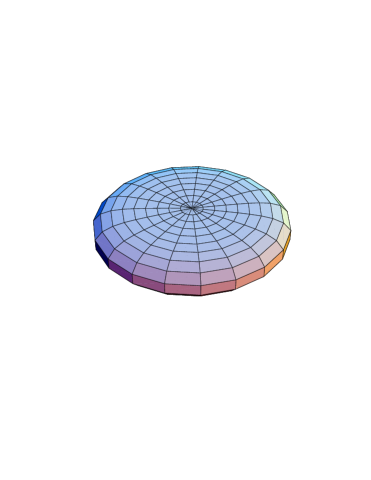
FIG. 9.: The spatial section of the weakly gravitating sine-Gordon domain wall. The surface shown is the $t^{*}=z^{*}=0$ surface for $\epsilon=1/30$.

The spatial geometry of the domain wall is therefore topologically $S^{3}$, and is similar to a discus, although the upper and lower surfaces are flat almost to the edge of the discus. This corresponds exactly to our intuitive idea of the spacetime exterior to the wall being flat, with a highly localised region of curvature generated by the wall itself located at the rim of the discus. It fleshes out the thin wall description of the spacetime, smoothing over the distributional singularity of the thin wall hypersurface. The two length scales of the domain wall spacetime correspond to the two radii of the discus, and as $\epsilon$ increases, the discus radius shrinks, with its height remaining much the same, until the geometry is almost spherical, at which point the radius becomes too small to support a defect solution and we make the transition to a false vacuum de Sitter hyperboloid, with an exactly spherical spatial geometry. What is interesting in comparison with the Avis and Isham scenario is that it is the self gravity of the domain wall which produces a compactification of spacetime at its own characteristic scale, which ultimately becomes too small to support the defect itself.

Finally, in analogy with [30], we can make a plot of the normalized action for the domain wall solution versus the de Sitter solution

$$S=\int{\cal L}_{\rm G}+{\cal L}_{\rm M}=\eta^{2}\int V(X)\,{\rm e}^{2kt}A^{3}d^{4}x=N\int_{0}^{z_{\rm h}}A^{3}V(X)dz,$$ (72)

where $N$ is a normalization factor, and there are no boundary terms from the gravitational part of the action. For the false vacuum de Sitter solution $\bar{S}=S/N=2/3k=2/\sqrt{3\epsilon}$, and for the weakly gravitating $\lambda\Phi^{4}$ model, ${\bar{S}}=2/3$. Figure 10 shows a plot of the action of the $\lambda\Phi^{4}$ wall against the false vacuum de Sitter solution, which indicates clearly the instability of the latter solution to wall formation for $\epsilon<3/2$. (This can be compared to the instanton action plot obtained in [21].)

FIG. 10.: Bifurcation diagram for the gravitating domain wall. We plot here the normalized action $\bar{S}$ as a function of $\epsilon$. Solid lines indicate the stable solutions found numerically, and the dashed line represents the unstable de Sitter solution.

REFERENCES

- [1] A.Vilenkin and E.P.S.Shellard, Cosmic strings and other topological defects (Cambridge: Cambridge University Press 1994)
- [2] A.Albrecht, R.A.Battye and J.Robinson, Phys. Rev. Lett. 79 4736 (1997). [astro-ph/9707129]
- [3] U.L.Pen, U.Seljak and N.Turok, Phys. Rev. Lett. 79 1611 (1997). [astro-ph/9704165]
- [4] P.Ferreira, J.Magueijo and K.M.Gorski, Astrophys. J. 503 L1 (1998). [astro-ph/9803256] J.Pando, D.Valls-Gabaud and L.Fang, Phys. Rev. Lett. 81 4568 (1998). [astro-ph/9810165] D.Novikov, H.Feldman and S.Shandarin, [astro-ph/9809238].
- [5] W.Israel, Nuovo Cim. 44B 1 (1966).
- [6] R.Gregory, Phys. Rev. D54 4955 (1996). [gr-qc/9606002]
- [7] A.Vilenkin, Phys. Lett. 133B 177 (1983).
- [8] J.Ipser and P.Sikivie, Phys. Rev. D30 712 (1984).
- [9] G.W.Gibbons, Nucl. Phys. B394 3 (1993).
- [10] D.Garfinkle and R.Gregory, Phys. Rev. D41 1889 (1990).
- [11] L.M.Widrow, Phys. Rev. D39 3571 (1989).
- [12] C.T.Hill, D.N.Schramm and J.N.Fry, Comm. Nucl. Part. Phys. 19 25 (1989).
- [13] G.Goetz, J. Math. Phys. 31 2683 (1990).
- [14] M.Mukherjee, Class. Quant. Grav. 10 131 (1993).
- [15] K.Tomita Phys. Lett. 244B 183 (1990).
- [16] S.Tadaki and H.Ishihara, Phys. Rev. D41 3047 (1990).
- [17] A.Linde, Phys. Lett. 237B 208 (1994). [astro-ph/9402031] A.Linde and D.Linde, Phys. Rev. D50 2456 (1994). [hep-ph/9402115]
- [18] A.Vilenkin, Phys. Rev. Lett. 72 3137 (1994). [hep-th/9402085]
- [19] R.Basu and A.Vilenkin, Phys. Rev. D50 7150 (1994). [gr-qc/9402040]
- [20] D.Boyanovsky, D.E.Brahm, A.Gonzalez-Ruiz, R.Holman and F.I.Takakura, Phys. Rev. D52 5516 (1995). [hep-ph/9501380]
- [21] R.Basu and A.Vilenkin, Phys. Rev. D46 2345 (1992).
- [22] R.Basu, A.H.Guth and A.Vilenkin, Phys. Rev. D44 340 (1991).
- [23] F.Bonjour, R.Emparan and R.Gregory, [gr-qc/9810061]
- [24] W.H.Press, S.A.Teukolsky, W.T.Vetterling and B.P.Flannery, Numerical recipes in C: The art of scientific computing, Second edition (Cambridge: Cambridge University Press 1992)
- [25] M.Cvetic, S.Griffies and H.H.Soleng, Phys. Rev. D48 2613 (1993). [gr-qc/9306005]
- [26] M.Cvetic and H.H.Soleng, Phys. Rep. 282 159 (1997). [hep-th/9604090]
- [27] M.Cvetic and S.Griffies, Phys. Lett. 285B 27 (1992). [hep-th/9204031]
- [28] N.Sakai, H.Shinkai, T.Tachizawa and K.Maeda, Phys. Rev. D53 655 (1996). Erratum Phys. Rev. D54 2981 (1996). [gr-qc/9506068]
- [29] A.Chamblin, J.M.A.Ashbourn-Chamblin, R.Emparan and A.Sornborger, Phys. Rev. Lett. 80 4378 (1998). [gr-qc/9706032] Phys. Rev. D58 124014 (1998). [gr-qc/9706004] F.Bonjour and R.Gregory, Phys. Rev. Lett. 81 5034 (1998). [hep-th/9809029]
- [30] S.J.Avis and C.J.Isham, Proc. Roy. Soc. Lond. A. 363 581 (1978).