Spinning C-metric: radiative spacetime with accelerating, rotating black holes

Abstract

The spinning C-metric was discovered by Plebański and Demiański as a generalization of the standard C-metric which is known to represent uniformly accelerated non-rotating black holes. We first transform the spinning C-metric into Weyl coordinates and analyze some of its properties as Killing vectors and curvature invariants. A transformation is then found which brings the metric into the canonical form of the radiative spacetimes with the boost-rotation symmetry. By analytically continuing the metric across “acceleration horizons”, two new regions of the spacetime arise in which both Killing vectors are spacelike.

We show that this metric can represent two uniformly accelerated, spinning black holes, either connected by a conical singularity, or with conical singularities extending from each of them to infinity. The radiative character of the metric is briefly discussed.

I Introduction

The static part of a spacetime representing the standard, non-spinning vacuum C-metric was originally found by Levi-Civita in 1917-1919 (see references in [1]) but it was only in 1970 when Kinnersley and Walker [2] understood, by choosing a better parameterization, that it can be extended so that it represents two black holes uniformly accelerated in opposite directions. The “cause” of the acceleration is given by nodal (conical) singularities (“strings” or “struts”) along the axis of symmetry. By adding an external gravitational field the nodal singularities can be removed [3]. If the holes are electrically (magnetically) charged the field causing the acceleration can be electric (magnetic) [4]. These types of generalized C-metric have been recently used in the context of quantum gravity - to describe production of black hole pairs in strong background fields (see, for example, [5], [6], [7]).

From the 1980’s several other works analyzed the standard C-metric. Ashtekar and Dray [8] were the first to show that the C-metric admits a conformal completion such that its null infinity admits spherical sections. Bonnor [9] transformed the vacuum C-metric to a Weyl form, in which the metric represents a “spherical particle” (in fact the horizon of the black hole) and a semi-infinite line mass, with a strut holding them apart. By another transformation Bonnor enlarged the spacetime so that it became “dynamic”, representing two black holes (“spherical particles” in terminology of [9]) uniformly accelerated by a spring joining them. In 1995 Cornish and Uttley [10] simplified Bonnor’s procedure and extended it to the charged case [11]. Most recently the black-hole uniqueness theorem for the C-metric has been proved [12].

In none of the above works, however, has the basic fact been emphasized that the vacuum C-metric is just one specific example in a large class of asymptotically flat radiative spacetimes with boost-rotation symmetry (with the boost along the axis of rotational symmetry). From a unified point of view, boost-rotation symmetric spacetimes with hypersurface orthogonal axial and boost Killing vectors were studied geometrically by Bičák and Schmidt [13]. We refer to this detailed work for rigorous definitions and theorems. In fact it is no surprise that the C-metric was for a long time analyzed in coordinate systems unsuitable for treating global issues such as the properties of null infinity. It is algebraically special, and the coordinate systems were adapted to its degenerate character. In polar coordinates $\{t,\ \rho,\ \phi,\ z\}$ the metric of a general boost-rotation symmetric spacetime with hypersurface orthogonal axial and boost Killing vectors,

$$\frac{\partial}{\partial\phi}\quad{\rm and}\quad z\frac{\partial}{\partial t}+t\frac{\partial}{\partial z}\ ,$$ (1)

has the form (see [13], Eq. (3.38)):

$${\rm d}s^{2}=e^{\lambda}{\rm d}\rho^{2}+\rho^{2}e^{-\mu}{\rm d}{\phi}^{2}+\frac{1}{z^{2}-t^{2}}\left((e^{\lambda}z^{2}-e^{\mu}t^{2}){\rm d}z^{2}-2zt(e^{\lambda}-e^{\mu}){\rm d}z{\rm d}t-(e^{\mu}z^{2}-e^{\lambda}t^{2}){\rm d}t^{2}\right)\ ,$$ (2)

where $\mu$ and $\lambda$ are functions of $\rho^{2}$ and $z^{2}-t^{2}$, satisfying, as a consequence of Einstein’s vacuum equations, a simple system of three equations, one of them being the wave equation for the function $\mu$. The whole structure of the group orbits in boost-rotation symmetric curved spacetimes outside the sources (or singularities) is the same as the structure of the orbits generated by the axial and boost Killing vectors in Minkowski space. In particular, the boost Killing vector (1) is timelike in the region $z^{2}>t^{2}$. It is this region which can be transformed to the static Weyl form. Physically this corresponds to the transformation to “uniformly accelerated frames” in which sources are at rest and the fields are time independent.

However, in the other “half” of the spacetime, $t^{2}>z^{2}$ (“above the roof” in the terminology of [13]), the boost Killing vector is spacelike so that in this region the metric (2) is nonstationary. It can be shown that for $t^{2}>\rho^{2}+z^{2}$ the metric can be locally transformed into the metric of the Einstein-Rosen waves. The radiative properties of the specific boost-rotation symmetric spacetime were investigated long ago [14], and for more general metrics in [15], [16], [17]. The boost-rotation symmetric spacetimes were used as tests beds in numerical relativity - see the review [18] for more details and references.

Now in all the work mentioned above it was assumed that the axial and boost Killing vectors are hypersurface orthogonal. Recently, Bičák and Pravdová [19] analyzed symmetries compatible with asymptotic flatness and admitting gravitational and electromagnetic radiation. They have shown that in axially symmetric electrovacuum spacetimes in which at least locally a smooth null infinity exists, the only second allowable symmetry which admits radiation is the boost symmetry. The axial and an additional Killing vector have not been assumed to be hypersurface orthogonal. In [19] the general functional forms of gravitational and electromagnetic news functions, and of the total mass of asymptotically flat boost-rotation symmetric spacetimes at null infinity have been obtained. However, until now no general theory similar to that given in [13] in the hypersurface orthogonal case is available for the boost-rotation symmetric spacetimes with Killing vectors which are not hypersurface orthogonal. Nevertheless there is one explicitly given metric which can be expected to serve as an example of these spacetimes - the spinning vacuum C-metric. It was discovered by Plebański and Demiański [20] in 1976, studied later by Farhoosh and Zimmerman [21], and very recently briefly discussed by Letelier and Oliveira [22]. In none of these works, however, was the boost-rotation character of the spacetime properly analyzed. In particular, “the canonical coordinates” in which the metric represents a generalization of the metric (2) so that global issues outside the sources could properly be studied have not been found so far.

The main purpose of this paper is to find such a representation of the spinning C-metric (SC-metric) which would generalize (2) and, thus, could also serve as a convenient example for building up the general theory of boost-rotation symmetric spacetimes with the Killing vectors which are in general not hypersurface orthogonal.

In the next section we first write the Plebański-Demiański class of metrics [20], specialized to the spinning vacuum case, discuss the ranges of parameters entering the metric and indicate the limiting procedure leading to the Kerr metric. In Section III the SC-metric is transformed into Weyl coordinates. This is not an easy task, fortunately we succeeded in generalizing the procedure Bonnor [9] used for the standard C-metric without spin. We show that, by choosing different values of the original Plebański-Demiański coordinates we can, in principle, arrive at various Weyl spacetimes.

The properties of Killing vectors and of some invariants of the Riemann tensor lead us, in section IV, to choose a physically plausible Weyl spacetime which contains both the black-hole and the acceleration horizon. Similarly as has been done with the standard C-metric [9], [10], we concentrate on this Weyl portion. In section V the metric is transformed into the “canonical form” of boost-rotation symmetric spacetimes with Killing vectors which need not be hypersurface orthogonal (see Eqs. (65)-(66)). By analytically continuing the resulting metric across the acceleration horizons (“the roof”), two new regions of spacetime arise as in the standard case of the C-metric without spin.

Let us emphasize that it is only now, after having described the spacetime in coordinates in which global issues can be addressed, that we are able to fix coordinates $t$, $\phi$ and two Killing vectors appropriately. The importance of this fact is briefly discussed in relation to the most recent work [22] in which a transformation to the canonical form was not performed. We also show that, analogous to the C-metric without spin, the axis of symmetry contains nodal singularities between the spinning “sources” (holes) which cause the acceleration, and is regular elsewhere; or the axis can be made regular between the sources but then the nodal singularities extend from each of the sources to infinity (see Fig. 4 a, b).

Finally, in our concluding remarks we briefly compare our results with those obtained recently in [22]. We then give two figures, constructed numerically, exhibiting clearly the radiative character of the SC-metric. A detailed analysis of the radiative properties of the SC-metric and of its analytic extension into the holes’ interiors will be given elsewhere.

II Spinning C-metric

Plebański and Demiański [20] gave their class of metrics in the coordinates $\{\tau$, $p$, $q$, $\sigma\}$ in the form

$${{\rm d}s}^{2}={\frac{E\left(Q-P{q}^{4}\right)}{F}}{{d\tau}}^{2}-{\frac{EF}{Q}}{{\rm d}q}^{2}-{\frac{EF}{P}}{{\rm d}p}^{2}+{\frac{E\left(Q{p}^{4}-P\right)}{F}}{{\rm d}\sigma}^{2}-{\frac{2\,E\left(Q{p}^{2}+P{q}^{2}\right)}{F}}{\rm d}\tau{\rm d}\sigma,$$ (3)

where

$$P = \gamma-{\varepsilon}\,{p}^{2}+2\,m{p}^{3}-\gamma{p}^{4}\ ,$$ (4)

$$Q = -\gamma+{\varepsilon}\,{q}^{2}+2\,m{q}^{3}+\gamma{q}^{4}\ ,$$ (5)

$$E = \left(p+q\right)^{-2}\ ,$$ (6)

$$F = 1+{p}^{2}{q}^{2}\ ,$$ (7)

$m$, $\gamma$, $\varepsilon$ being constants. The choice of the exact ranges of dimensionless coordinates $p$, $q$ will be specified later, at this point we consider $p$, $q$ $\in$ $R$; the coordinates $\tau$, $\sigma$ have dimension of $($length$)^{2}$, and we also take $\tau$, $\sigma$ $\in R$. In the general form of Plebański-Demiański metric (Eqs. (2.1), (3.25) in [20]) we put the parameters $n$, $e$, $g$, $\lambda$, corresponding to the NUT parameter, electric and magnetic charge, and cosmological constant, equal to zero. If parameter $m=0$ the spacetime is flat. It is not straightforward to obtain standard metrics from (3). In [20] it is shown (see also [1]) that the stationary (non-accelerated) Kerr solution can be obtained by scaling the coordinates and, simultaneously, the parameters as

$$p=\frac{p^{\prime}}{l}\ ,\ \ q=\frac{-l}{q^{\prime}}\ ,\ \ \tau={l}{\tau^{\prime}}\ ,\ \ \sigma={l^{3}}{\sigma^{\prime}}\ ,$$

$$m={l^{-3}}{m^{\prime}}\ ,\ \ \varepsilon={l^{-2}}{\varepsilon^{\prime}}\ ,\ \ \gamma={l^{-4}}{\gamma^{\prime}}\ .$$ (8)

Then, after taking the limit $l\rightarrow\infty$ and putting

$$m^{\prime}=M\ ,\ \ \varepsilon^{\prime}=1\ ,\ \ \gamma^{\prime}=a^{2}\ ,\ \ p^{\prime}=-a\cos\theta\ ,\ \ q^{\prime}=r\ ,\ \ \sigma^{\prime}=-\phi/a\ ,\ \ \tau^{\prime}=t+a\phi\ ,$$ (9)

we obtain the standard Kerr metric with mass $M$ and specific angular momentum $a$ in the Boyer-Lindquist coordinates. If $\varepsilon=m^{2}/\gamma$, the limiting procedure leads to the extreme Kerr hole with $a^{2}=M^{2}$. It is worth noticing that in this case the quartic $P$ can be factorized, $P=-{\gamma}^{-1}(\gamma p^{2}-mp+\gamma)(\gamma p^{2}-mp-\gamma)$. If $\varepsilon>m^{2}/\gamma$, we obtain a general Kerr black hole; with $\varepsilon<m^{2}/\gamma$ - a Kerr naked singularity. Another limiting procedure (see [20], [1]) leads to the C-metric without rotation.

In the following we shall restrict ourselves to the general case in which the polynomials (4) and (5) have four different real roots. We thus omit the special cases which may be of interest (cf. [8], [23]) but will be dealt with elsewhere. Notice that if $p_{i}$ is the root of the polynomial $P$ given by Eq. (4), then $q_{i}=-p_{i}$ is the root of the polynomial $Q$ (Eq. (5)). The analysis of the 4th-order polynomial (5) shows that if $\gamma$ is chosen positive, the polynomial has four different roots provided that

$$\epsilon > 2\sqrt{3}\gamma\ ,$$ (10)

$$\frac{\epsilon(\epsilon^{2}+36\gamma^{2})-(\epsilon^{2}-12\gamma^{2})^{3/2}}{54\gamma}< m^{2} <\frac{\epsilon(\epsilon^{2}+36\gamma^{2})+(\epsilon^{2}-12\gamma^{2})^{3/2}}{54\gamma}\ .$$ (11)

In Fig. 1 we illustrate the allowed range of the parameters for $\gamma=1$.

FIG. 1.: The allowed range of parameters $\varepsilon$ and $m^{2}$ for $\gamma=1$. If a point $(\varepsilon,m^{2})$ is “between” the two curves, then both polynomials $P,Q$ have four distinct real roots.

Returning back to the metric (3) - (7), we immediately observe that it has two Killing vectors,

$${\frac{\partial}{\partial\tau}}\quad{\rm and}\quad{\frac{\partial}{\partial\sigma}}\ .$$ (12)

III SC-metric in Weyl coordinates

We just saw that the SC-metric has two Killing vectors (12). We also noticed that in a limit it goes over into the C-metric without rotation (cf. [1]) which is known to be axisymmetric and in some regions static. Hence, we expect that the SC-metric can be converted into a standard Weyl-Papapetrou form

$${\rm d}s^{2}={\rm e}^{-2U}\left({{\rm e}^{2\nu}}({{\rm d}\bar{\rho}}^{2}+{{{\rm d}\bar{z}}}^{2})+{\bar{\rho}}^{2}{{{\rm d}\bar{\varphi}}}^{2}\right)-{{\rm e}^{2\,U}}\left({{\rm d}\bar{t}}+A{{\rm d}\bar{\varphi}}\right)^{2}\ ,$$ (13)

where functions $U$, $\nu$, $A$ depend only on $\bar{\rho}$ and $\bar{z}$, $\bar{\varphi}\in\langle 0,2\pi)$, $\bar{\rho}\in\langle 0,\infty)$, $\bar{t},\bar{z}\in R$.

Vacuum Einstein’s equations imply

$$\frac{\partial^{2}U}{\partial\bar{z}^{2}}+\frac{1}{\bar{\rho}}\frac{\partial U}{\partial\bar{\rho}}+\frac{\partial^{2}U}{\partial\bar{\rho}^{2}}=-\frac{1}{2}\frac{{\rm e}^{4U}}{\bar{\rho}^{2}}\left[\left(\frac{\partial A}{\partial\bar{\rho}}\right)^{2}+\left(\frac{\partial A}{\partial\bar{z}}\right)^{2}\right]\ ,$$ (14)

$$\frac{\partial}{\partial\bar{z}}\left(\frac{{\rm e}^{4U}}{\bar{\rho}}\frac{\partial A}{\partial\bar{z}}\right)+\frac{\partial}{\partial\bar{\rho}}\left(\frac{{\rm e}^{4U}}{\bar{\rho}}\frac{\partial A}{\partial\bar{\rho}}\right)=0\ ,$$ (15)

$$\frac{1}{\bar{\rho}}\frac{\partial\nu}{\partial\bar{\rho}}=\left(\frac{\partial U}{\partial\bar{\rho}}\right)^{2}-\left(\frac{\partial U}{\partial\bar{z}}\right)^{2}-\frac{{\rm e}^{4U}}{4\bar{\rho}^{2}}\left[\left(\frac{\partial A}{\partial\bar{\rho}}\right)^{2}-\left(\frac{\partial A}{\partial\bar{z}}\right)^{2}\right]\ ,$$ (16)

$$\frac{1}{\bar{\rho}}\frac{\partial\nu}{\partial\bar{z}}=2\frac{\partial U}{\partial\bar{\rho}}\frac{\partial U}{\partial\bar{z}}-\frac{{\rm e}^{4U}}{2\bar{\rho}^{2}}\frac{\partial A}{\partial\bar{\rho}}\frac{\partial A}{\partial\bar{z}}\ .$$ (17)

Axial and timelike Killing vectors

$$\xi_{(\bar{\varphi})}=\frac{\partial}{\partial\bar{\varphi}}\ ,\ \xi_{(\bar{t})}=\frac{\partial}{\partial\bar{t}}\ ,$$ (18)

determine invariantly the cylindrical-type radial coordinate by the relation

$${\bar{\rho}}^{2}={g_{\bar{t}\bar{\varphi}}}^{2}-{g_{\bar{t}\bar{t}}}\,{g_{\bar{\varphi}\bar{\varphi}}}\ =\ (\xi_{(\bar{t})},\xi_{(\bar{\varphi})})^{2}-(\xi_{(\bar{t})},\xi_{(\bar{t})})(\xi_{(\bar{\varphi})},\xi_{(\bar{\varphi})})\ .$$ (19)

In the following we shall consider points with $\bar{\rho}=0$ as “lying on the $\bar{z}$-axis of axial symmetry”. This is indeed the axis of Weyl’s coordinates, however, it must be born on mind that $\bar{\rho}=0$ is a real smooth geometrical (physical) axis only there where the metric (13) satisfies the regularity conditions

$$\lim_{\bar{\rho}\to\infty}\frac{X_{,\alpha}X^{,\alpha}}{4X}=1\ ,\ {\rm where}\ X=\xi_{(\bar{\varphi})\alpha}\xi_{(\bar{\varphi})}^{\alpha}\ ,\ \ \alpha=0-3.$$ (20)

We shall see that for some intervals of $\bar{z}$ the points $\bar{\rho}=0$ may represent either a horizon of a rotating black hole or a rotating string - regularity conditions (20) are then not satisfied. The norms of the Killing vectors will enable us to distinguish between horizons and strings.

In order to convert the original metric (3)-(7) into the Weyl-Papapetrou metric (13), we shall seek the transformation of the form

$$\bar{\rho}=\bar{\rho}(p,q)\ ,\ \ \bar{z}=\bar{z}(p,q)\ ,\ \ \bar{t}=\bar{t}(\tau,\sigma)\ ,\ \ \bar{\varphi}=\bar{\varphi}(\tau,\sigma)\ .$$ (21)

Since the Killing vectors (12) must be linear combinations with constant coefficients of the Killing vectors (18), we can write

$${d\tau}={\kappa_{1}}\,{d\bar{t}}+{\kappa_{2}}\,{d\bar{\varphi}}\ ,$$ (22)

$${d\sigma}={\kappa_{3}}\,{d\bar{t}}+{\kappa_{4}}\,{d\bar{\varphi}}\ ,$$ (23)

with $\kappa_{1}\dots\kappa_{4}$ constants. As a consequence of (21) and (23) we find the metric components associated with the Killing vectors to be given in Weyl coordinates by

$$g_{\bar{\varphi}\bar{\varphi}} = \frac{E}{F}\left(\left(-\kappa_{2}+p^{2}\kappa_{4}\right)^{2}Q-\left(\kappa_{4}+q^{2}\kappa_{2}\right)^{2}P\right)\ ,$$ (24)

$$g_{\bar{\varphi}\bar{t}} = \frac{E}{F}\left(\left(-{\kappa_{1}}+{p}^{2}{\kappa_{3}}\right)\left(-{\kappa_{2}}+{p}^{2}{\kappa_{4}}\right)Q-\left({\kappa_{3}}+{q}^{2}{\kappa_{1}}\right)\left({\kappa_{4}}+{q}^{2}{\ \kappa_{2}}\right)P\right)\ ,$$ (25)

$$g_{\bar{t}\bar{t}} = \frac{E}{F}\left(\left(-{\kappa_{1}}+{p}^{2}{\kappa_{3}}\right)^{2}Q-\left({\kappa_{3}}+{q}^{2}{\kappa_{1}}\right)^{2}P\right)\ .$$ (26)

Substituting these components into Eq. (19), we arrive at surprisingly simple expression for $\bar{\rho}$:

$$\bar{\rho}^{2}={E}^{2}{\cal K}^{2}PQ\ ,\ \ \ {\cal K}=\left({\kappa_{2}}\,{\kappa_{3}}-{\kappa_{1}}\,{\kappa_{4}}\right)\ .$$ (27)

Notice that this result is in a disagreement with the last Eq. (34) of [22]; there only the first term should appear.

Turning now to the transformation of variables $p$, $q$ into Weyl’s $\bar{\rho}$, $\bar{z}$, we first write

$${d\bar{\rho}}={\cal A}{dp}+{\cal B}{dq}\ ,$$ (28)

$${d\bar{z}}={\cal C}{dp}+{\cal D}{dq}\ .$$ (29)

Functions ${\cal A}$ and ${\cal B}$ can be determined from Eq. (27). Functions ${\cal C}$ and ${\cal D}$ can be obtained by inverting relations (29), substituing into the original metric (3) and demanding that $g_{\bar{\rho}\bar{\rho}}=g_{\bar{z}\bar{z}}$, $g_{\bar{\rho}\bar{z}}=0$. In this way we find

$${\cal A}={\cal K}\frac{\partial}{\partial p}\left(E{\sqrt{PQ}}\right)\ \quad{\cal B}={\cal K}\frac{\partial}{\partial q}\left(E{\sqrt{PQ}}\right)\ ,$$ , (30)

$${\cal C}=\mp{\frac{{\cal B}\sqrt{QP}}{P}}\ \quad{\cal D}=\pm{\frac{{\cal A}\sqrt{QP}}{Q}}\ .$$ , (31)

Since ${\cal C}=\partial\bar{z}/\partial p$, ${\cal D}=\partial\bar{z}/\partial q$, and the integrability conditions $\partial{\cal C}/\partial q-\partial{\cal D}/\partial p=0$ are satisfied, we can integrate for $\bar{z}$. Regarding Eqs. (4) - (7) we obtain

$$\bar{z}=\mp|{\cal K}|\left({\frac{-\gamma-{\varepsilon}\,qp-m{q}^{2}p+mq{p}^{2}+\gamma{q}^{2}{p}^{2}}{\left(p+q\right)^{2}}}\right)\ ,$$ (32)

where we put an additive constant equal to zero. We thus arrive at the metric functions determining the Weyl-Papapetrou line element (13) in the form:

$${\rm e}^{2U} = -g_{\bar{t}\bar{t}}\ ,$$ (33)

$${\rm e}^{2\nu} = -g_{\bar{\rho}\bar{\rho}}g_{\bar{t}\bar{t}}\ ,$$ (34)

$$A = \frac{g_{\bar{t}\bar{\varphi}}}{g_{\bar{t}\bar{t}}}\ ,$$ (35)

where

$$g_{\bar{\rho}\bar{\rho}}=g_{\bar{z}\bar{z}}=-\frac{EF}{A^{2}P+B^{2}Q}\ ,$$ (36)

and $g_{\bar{t}\bar{t}}$, $g_{\bar{t}\bar{\varphi}}$ are given by Eqs. (26). In this way we succeeded in expressing the Weyl metric functions in terms of $p$, $q$.

In order to find these functions directly in the Weyl coordinates, we have to invert relations (see Eqs. (27), (32) and (4), (5))

$$\bar{z} = {\cal K}{\frac{-\gamma-\varepsilon\,qp-m{q}^{2}p+mq{p}^{2}+\gamma{q}^{2}{p}^{2}}{(p+q)^{2}}}\ ,$$ (37)

$${\bar{\rho}}^{2} = {\frac{{\cal K}^{2}(\gamma-{\varepsilon}\,{p}^{2}+2\,m{p}^{3}-\gamma{p}^{4})(-\gamma+{\varepsilon}\,{q}^{2}+2\,m{q}^{3}+\gamma{q}^{4})}{(p+q)^{4}}}\ .$$ (38)

This is not an easy task. Fortunately, we can try to generalize the procedure used by Bonnor [9] for the vacuum C-metric without rotation (see Eq. (11) in [9]). We thus wish to find constants $\alpha_{1}$, $\alpha_{2}$, $\alpha_{3}$, $\alpha_{4}$ and $z_{i}$, $i=1,\ 2,\ 3$, such that

$$\bar{\rho}^{2}+(\bar{z}-{\bar{z}_{i}})^{2}=\Bigl{(}\frac{{\alpha_{1}}p+{\alpha_{2}}q+{\alpha_{3}}+{\alpha_{4}}pq}{p+q}\Bigr{)}^{2}\ .$$ (39)

Multiplying the last equation by $(p+q)^{2}$, regarding expressions (37), (38), and requiring the coefficients in the resulting polynomial to vanish, we get

$${\alpha_{1}}=-W_{i}\ ,\quad{\alpha_{2}}=W_{i}\ ,\quad{\alpha_{3}}=\frac{{\cal K}^{2}m\gamma}{W_{i}}\ ,\quad{\alpha_{4}}=\frac{{\cal K}m\bar{z}_{i}}{W_{i}}\ ,$$ (40)

where $\bar{z}_{i}/{\cal K}$ are the roots of the equation

$$2(\bar{z}_{i}/{\cal K})^{3}+\varepsilon(\bar{z}_{i}/{\cal K})^{2}+2\gamma^{2}(\bar{z}_{i}/{\cal K})+\varepsilon\gamma^{2}-m^{2}\gamma=0\ ,\ \ i=1,\ 2,\ 3,$$ (41)

and

$$W_{i}=\sqrt{{\cal K}^{2}{\gamma}^{2}+{\bar{z}_{i}}^{2}}\ .$$ (42)

Next we introduce functions

$$R_{i}={\sqrt{\bar{\rho}^{2}+(\bar{z}-{\bar{z}_{i}})^{2}}\ \geq\ 0\ .}$$ (43)

After substituting for $\alpha_{1}\dots\alpha_{4}$ from Eq. (40) into the relation (39) and taking square roots, we can rewrite the functions $R_{i}$ in the form

$$R_{i}=\epsilon_{i}\frac{1}{(p+q)}\left(-W_{i}p+W_{i}q+\frac{{\cal K}^{2}m\gamma}{W_{i}}+\frac{{\cal K}m\bar{z}_{i}pq}{W_{i}}\right)\ ,$$ (44)

in which $\epsilon_{i}$ is chosen $+1$ or $-1$ so that the right-hand side of (44) is indeed positive. Eq. (44) represents three dependent equations for $p$ and $q$ as functions of $\bar{\rho}$ and $\bar{z}$. These can be easily solved if first simple new variables such as, for example, $pq$, $p+q$, $-p+q$ are introduced. Finally we succeed to express $p$ and $q$ as follows:

$$p = \frac{S_{1}-S_{2}}{2S_{3}}\ ,$$ (45)

$$q = \frac{S_{1}+S_{2}}{2S_{3}}\ ,$$ (46)

where

$$S_{1} = -\epsilon_{1}\epsilon_{2}\epsilon_{3}{\cal K}^{2}m\gamma(\bar{z}_{1}-\bar{z}_{2})(\bar{z}_{1}-\bar{z}_{3})(\bar{z}_{2}-\bar{z}_{3})\ ,$$ (47)

$$S_{2} = \gamma m{\cal K}^{2}\left(\epsilon_{2}\epsilon_{3}(\bar{z}_{3}-\bar{z}_{2})W_{1}R_{1}+\epsilon_{1}\epsilon_{3}(\bar{z}_{1}-\bar{z}_{3})W_{2}R_{2}-\epsilon_{1}\epsilon_{2}(\bar{z}_{1}-\bar{z}_{2})W_{3}R_{3}\right)\ ,$$ (48)

$$S_{3} = -\epsilon_{2}\epsilon_{3}(\bar{z}_{3}-\bar{z}_{2})({\cal K}^{2}\gamma^{2}-\bar{z}_{2}\bar{z}_{3})W_{1}R_{1}+\epsilon_{1}\epsilon_{3}(\bar{z}_{3}-\bar{z}_{1})({\cal K}^{2}\gamma^{2}-\bar{z}_{1}\bar{z}_{3})W_{2}R_{2}$$ (50)

$$+\epsilon_{1}\epsilon_{2}(\bar{z}_{1}-\bar{z}_{2})({\cal K}^{2}\gamma^{2}-\bar{z}_{1}\bar{z}_{2})W_{3}R_{3}\ .$$

Therefore, by choosing different values for $\epsilon_{i}$ in the last expressions, we arrive at different $p$’s and $q$’s according to relations (46) and, thus, to different Weyl metric functions (33) - (35). Because there exist eight different choices for $\epsilon_{i}$ we get in principle eight different Weyl spacetimes. Their properties will be analyzed in the next section. As we shall see, only four of them have the signature $+2$, which we are using in this paper.

IV Properties of the SC-metric in $(p,q)$ and $(\bar{\rho},\bar{z})$ coordinates

First we shall study the character of the Killing vectors. In particular we seek a region of spacetime in which there exists a linear combination (with constants coefficients $k_{1},k_{2}$) of Killing vectors,

$$\eta=k_{1}\frac{\partial}{\partial\tau}+k_{2}\frac{\partial}{\partial\sigma}\ ,$$ (51)

which is spacelike, and another combination which is timelike so that the region is then stationary. Hence, the quadratic form

$$g_{\alpha\beta}\eta^{\alpha}\eta^{\beta}=k_{1}^{2}g_{\tau\tau}+2k_{1}k_{2}g_{\tau\sigma}+k_{2}^{2}g_{\sigma\sigma}$$ (52)

must there be indefinite. This implies that the matrix $g_{AB}$, $A,\ B=\tau,\sigma,$ (given by Eqs. (3) - (7)) has eigenvalues $\lambda_{1},\lambda_{2}$ satisfying $\lambda_{1}\lambda_{2}<0$. Since it turns out that

$$\lambda_{1}\lambda_{2}=-E^{2}PQ\ ,$$ (53)

the stationary regions are those in which

$$PQ>0\ .$$ (54)

The analysis of the eigenvalues $\lambda_{1},\lambda_{2}$ reveals that $\lambda_{1}+\lambda_{2}=-(E/F)(P(1+q^{4})-Q(1+p^{4}))$ and since sign($\lambda_{1}\lambda_{2}$) = $-$sign($PQ$), we find out that the metric (3) has the signature $-2$ if $P>0$, whereas $P<0$ implies signature $+2$. Since in this paper we are choosing the signature $+2$, we take $P<0$.

The character of the regions described by the specific intervals of $(p,q)$ coordinates is best understood by plotting them in the schematic Figure 2. Here $p_{1}<p_{2}<p_{3}<p_{4}$ and $q_{1}<q_{2}<q_{3}<q_{4}$ denote the roots of the polynomials $P$ and $Q$, the numbers $1,\ \dots,\ 5$ indicate regions between individual roots or between a root and infinity. Notice that the Figure is schematic in the sense that the squares are plotted to have the same size, even though the lengths of the intervals between the roots are not the same.

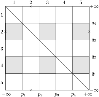
FIG. 2.: The schematic illustration of the character of the regions described by the specific intervals of $(p,q)$ coordinates. See the text for the details.

Now in the polynomials $P$, $Q$ we choose, without loss of generality, parameter $\gamma>0$. Since our signature $+2$ requires $P<0$, we consider only the squares in the columns $1,\ 3,\ 5.$ In the squares which represent stationary regions, the inequality (54) is valid - in Fig. 2 these squares are shaded. By numerically analyzing the right-hand side of Eq. (44) we can make sure that in the squares $\{2,1\}$ and $\{2,5\}$ all parameters $\epsilon_{i}=-1$, in $\{4,1\}$ and $\{4,5\}$, $\epsilon_{1}=\epsilon_{2}=1$, $\epsilon_{3}=-1$, in $\{4,3\}$, $\epsilon_{1}=\epsilon_{3}=1$, $\epsilon_{2}=-1$ and in the square $\{2,3\}$, which will play the main role in the following, we find $\epsilon_{1}=-1$, $\epsilon_{2}=\epsilon_{3}=1$.

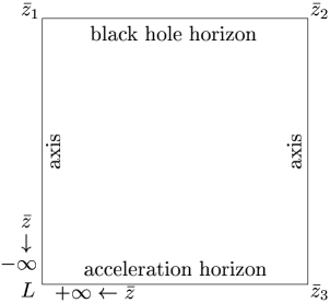
FIG. 3.: The square $\{2,3\}$, with $p\in\langle p_{2},p_{3}\rangle$, $q\in\langle q_{3},q_{4}\rangle.$ The locations of infinity, the axis, and the black-hole and acceleration horizon are indicated. See the text for the details.

The shaded square $\{2,3\}$ is illustrated in detail in Fig. 3. The boundaries of the square represent the axis $\bar{\rho}=0$ because of the relation (27). The transformation (37) implies that the vortices of the square correspond to the roots $\bar{z}_{i}$ of the equation (41). From the same transformation (37) we also see that the lower left vortex $L$ (corresponding to $p_{2},\ q_{3}$) is special: when it is approached along two different edges of the square we arrive at either $\bar{z}\rightarrow+\infty$ or $\bar{z}\rightarrow-\infty$. In addition, by approaching this vortex along different lines from the interior of the squares we can achieve various values of $\bar{z}$ and $\bar{\rho}$.

Since the character of the Killing vectors depends on the eigenvalues $\lambda_{1}$, $\lambda_{2}$ (cf. Eqs. (52), (53)), and on the boundaries of the square either $\lambda_{1}=0$ or $\lambda_{2}=0$, just one of the Killing vectors has to be null there. Between $\bar{z}_{1}$ and $\bar{z}_{2}$ all other Killing vectors are spacelike so that this part of the axis will describe the Killing horizon, the same being true for the boundary between $L$ and $\bar{z}_{3}$. Later we shall see that the segment between $\bar{z}_{1}$ and $\bar{z}_{2}$ corresponds to the black-hole horizon whereas that between $L$ and $\bar{z}_{3}$ to the acceleration horizon. The remaining segments, between $\bar{z}_{1}$ and $L$, and $\bar{z}_{2}$ and $\bar{z}_{3}$, describe the axis of symmetry, $\bar{\rho}=0$, along which, however, may lay the string represented by a conical singularity. There exists just one combination (51) of the Killing vectors (corresponding to the minimum of the quadratic form (52)) the norm of which is null, all other combinations (51) give timelike vectors.

It is useful to calculate several simplest invariants of the Riemann tensor for the metric (3):

$$I_{1} = {R^{\alpha\beta}}_{\gamma\delta}{R_{\alpha\beta}}^{\gamma\delta}=-48m^{2}\frac{(q^{6}p^{6}-15q^{4}p^{4}+15q^{2}p^{2}-1)(p+q)^{6}}{(1+p^{2}q^{2})^{6}}\ ,$$ (55)

$$I_{2} = {R^{\alpha\beta}}_{\gamma\delta}{R^{\gamma\delta}}_{\varepsilon\lambda}{R^{\varepsilon\lambda}}_{\alpha\beta}=96m^{3}\frac{(9q^{8}p^{8}-84q^{6}p^{6}+126q^{4}p^{4}-36p^{2}q^{2}+1)(p+q)^{9}}{(1+p^{2}q^{2})^{9}}\ ,$$ (56)

$$I_{3} = R^{\alpha\beta\gamma\delta}R_{\alpha\varepsilon\lambda\mu}{R^{\varepsilon\lambda}}_{\beta\nu}{R^{\mu\nu}}_{\gamma\delta}=-144m^{4}\frac{(p+q)^{12}}{(1+p^{2}q^{2})^{6}}\ .$$ (57)

Curiously, it is the last invariant which most simply indicates that asymptotically flat regions can exist only on the line given by

$$p+q=0\ .$$ (58)

On this line invariants $I_{1}$ and $I_{2}$ also vanish. In Section V, where the “canonical coordinates” will be introduced, we shall see that indeed the point $L$ in Fig. 3 corresponds to “points at infinity” where the spacetime is flat. The invariants (56) diverge at the points

$$[p,q]=[0,\infty],\ [0,-\infty],\ [-\infty,0],\ [\infty,0],$$ (59)

which thus correspond to curvature singularities.

The region $\{2,3\}$ described above appears to be most plausible from physical point of view to represent a uniformly accelerated, rotating black hole. We shall use this region in the following. The regions $\{2,1\}$, $\{2,5\}$ which also give signature $+2$ and contain a timelike Killing vector, imply the existence of a naked singularity. Indeed, the invariants (56) diverge at the point $[p=-\infty,q=0]$ which lies in the left edge of $\{2,1\}$, and at the point $[p=\infty,q=0]$ in the right edge of $\{2,5\}$. In fact one can make sure that by gluing these to edges together (and thus identifying the singular points) both regions $\{2,1\}$ and $\{2,5\}$ glued together will give one Weyl space. (Notice that $\epsilon_{1}$, $\epsilon_{2}$ and $\epsilon_{3}$ are the same in these regions.) Since, however, it contains a singular ring at $\bar{\rho}\not=0$ (corresponding to the identified singular points at the edges) we shall not consider these regions further. We shall see in the next section that the region $\{2,3\}$, after appropriate transformation and extension, gives the required form of the boost-rotation symmetric spacetime with Killing vectors which are not hypersurface orthogonal.

V The SC-metric in the canonical coordinates adapted to the boost-rotation symmetry

Following Bonnor’s analysis [9] of the standard C-metric we now make the transformation from the Weyl coordinates to new coordinates in which the boost-rotation symmetry of the SC-metric will become manifest. Simultaneously, by analytically continuing the resulting metric, two new regions of spacetime will arise - in a close analogy to the C-metric without spin. The transformation

$$\bar{t} = {\rm arctanh}\frac{t}{z}\ ,$$ (60)

$$\bar{\rho} = \rho\sqrt{z^{2}-t^{2}}\ ,$$ (61)

$$\bar{z}-\bar{z}_{3} = \frac{1}{2}\left(\rho^{2}+t^{2}-z^{2}\right)\ ,$$ (62)

$$\bar{\varphi} = \varphi\ ,$$ (63)

brings the metric (13) into the form

$${\rm ds}^{2}={\rm e}^{\lambda}{\rm d}\rho^{2}+\rho^{2}{\rm e}^{-\mu}{\rm d}\varphi^{2}+\frac{1}{z^{2}-t^{2}}\left[({\rm e}^{\lambda}z^{2}-{\rm e}^{\mu}t^{2}){\rm d}z^{2}-2zt({\rm e}^{\lambda}-{\rm e}^{\mu}){\rm d}z{\rm d}t+({\rm e}^{\lambda}t^{2}-{\rm e}^{\mu}z^{2}){\rm d}t^{2}\right]$$ (64)

$$-2A{\rm e}^{\mu}(z{\rm d}t-t{\rm d}z){\rm d}\varphi-A^{2}{\rm e}^{\mu}(z^{2}-t^{2}){\rm d}\varphi^{2}\ ,$$ (65)

where

$${\rm e}^{\mu}=\frac{{\rm e}^{2U}}{z^{2}-t^{2}}\ ,\quad{\rm e}^{\lambda}=\frac{{\rm e}^{2\nu}}{{\rm e}^{2U}}(\rho^{2}+z^{2}-t^{2})\ ,$$ (66)

and functions ${\rm e}^{2U}$, ${\rm e}^{2\nu}$ and $A$ are given in terms of coordinates $\{t,\rho,z,\varphi\}$ by Eqs. (26), (33)-(36), (41)-(43), (46), (50) and (61). One can easily obtain the transformation inverse to (61) in the form

$$t = \pm\sqrt{\sqrt{\bar{\rho}^{2}+(\bar{z}-\bar{z}_{3})^{2}}-(\bar{z}-\bar{z}_{3})}\sinh\bar{t}\ ,$$ (67)

$$\rho = \sqrt{\sqrt{\bar{\rho}^{2}+(\bar{z}-\bar{z}_{3})^{2}}+(\bar{z}-\bar{z}_{3})}\ ,$$ (68)

$$z = \pm\sqrt{\sqrt{\bar{\rho}^{2}+(\bar{z}-\bar{z}_{3})^{2}}-(\bar{z}-\bar{z}_{3})}\cosh\bar{t}\ ,$$ (69)

where either upper signs or lower signs are valid.

The form (65) represents a general boost-rotation symmetric spacetime “with rotation”, i.e., with the Killing vectors which are not hypersurface orthogonal. Putting $A=0$, we recover the canonical form of the boost-rotation symmetric spacetimes with the hypersurface orthogonal Killing vectors the general structure of which was studied in [13] . Notice that transformation (61) is meaningful only for $z^{2}>t^{2}$, i.e., “below the roof”, using the terminology of [13]. Here it leads to the explicit forms of metric functions ${\rm e}^{\mu}$, ${\rm e}^{\lambda}$, and $A$. Assuming then that these functions are analytically continued across the roof $z^{2}=t^{2}$ and across the null cone $z^{2}+\rho^{2}-t^{2}=0$, we find out that, by choosing the coefficients $\kappa_{1}$, $\kappa_{2}$, $\kappa_{3}$, $\kappa_{4}$ in the relation (23) appropriately, the metric can be made smooth across both the roof and null cone except for the axis $\rho=0$ in general, as will be seen in the following. (In the original coordinates $\{\tau,p,q,\sigma\}$ the region $t^{2}>z^{2}$ corresponds to the square $\{3,3\}$ in Fig. 2.) In addition, as a consequence of transformation (61), (68), we now get two rotating black holes uniformly accelerated in opposite directions, instead of one represented in the original Weyl coordinates, since the transformation (68) with the upper signs transforms the Weyl region into the region with $z^{2}>t^{2}$, $z>0$, whereas that with the lower signs into $z^{2}>t^{2}$, $z<0$ (see Fig. 4 and discussion below).

In order to choose the coordinates $\bar{t}$, $\bar{\varphi}$, $t$, $\varphi$ and the Killing vectors appropriately, i.e., to fix constants $\kappa_{1}\dots\kappa_{4}$ in the relation (23), we analyze the behaviour of the metric at spacelike infinity. This is simpler to do in the original coordinates $p$, $q$ where we look for a curve approaching

$$\rho\rightarrow\infty\ ,\ \ \varphi\rightarrow{\rm{const}},\ \ z\rightarrow{\rm{const}}\ ,\ \ t\rightarrow{\rm{const}}\ ,\ \ z^{2}>t^{2}\ .$$ (70)

In Weyl’s coordinates this can be achieved by choosing a parameter $v$ and putting $\bar{\rho}=v$, $\bar{z}=v^{2}$, $\bar{t}=$const, $\bar{\varphi}=$const, with $v\rightarrow\infty$. In the coordinates $p$, $q$ we can choose, correspondingly, the curve

$$p=p_{2}+v^{-2}\ ,\quad q=-p_{2}+v^{-4}\ ,$$ (71)

$p_{2}$ being the root of $P$, with $v\rightarrow\infty$. This curve approaches the point $L$ in Fig. 3. Regarding the transformation (37), (38), we see that indeed $\bar{\rho}\sim v$, $\bar{z}\sim v^{2}$, $\bar{t}=$const, $\bar{\varphi}=$const, as required.

In order to obtain spacetimes which are asymptotically Minkowskian along the curve (70), we now require

$${\rm e}^{\mu}\rightarrow 1\ ,\quad{\rm e}^{\lambda}\rightarrow 1\ ,\quad A\rightarrow 0$$ (72)

for (70), i.e., along the curve (71) with $v\rightarrow\infty$. The explicit form of $g_{\bar{\rho}\bar{\rho}}$, given in (36), when expressed along the curve (71), leads to $g_{\bar{\rho}\bar{\rho}}={\rm e}^{2\nu}/{\rm e}^{2U}\sim v^{-2}\sim\bar{\rho}^{-2}$. The requirement (72) rewritten in terms of functions $U$ and $\nu$, leads to ${\rm e}^{2U}\rightarrow$ const, ${\rm e}^{2\nu}\sim\bar{\rho}^{-2}\sim\rho^{-2}$ (cf. Eqs. (61), (66)); it is thus satisfied if ${\rm e}^{2U}\rightarrow$ const. This implies, using Eqs. (33) and (26), the following relation for the coefficients $\kappa_{3}$ and $\kappa_{1}$:

$$\kappa_{3}=-p_{2}^{2}\kappa_{1}.$$ (73)

Similarly, requiring $A\rightarrow 0$ along the curve (70), we deduce from Eqs. (35) and (26) the relation for $\kappa_{2}$ and $\kappa_{4}$:

$$\kappa_{2}=p_{2}^{2}\kappa_{4}.$$ (74)

Until now we considered the region $z^{2}>t^{2}$, i.e., “bellow the roof”. Turning to the roof itself, the necessary condition of the regularity of the metric there reads (cf. the detailed discussion in Section V in [13] in the case of the hypersurface orthogonal Killing vectors)

$${\rm e}^{\lambda}{\rm e}^{-\mu}=1\quad{\rm at}\quad z^{2}=t^{2}\ .$$ (75)

Eq. (66) then implies

$$\frac{{\rm e}^{2\nu}}{{\rm e}^{4U}}\bar{\rho}^{2}\rightarrow 1\ \ {\rm for}\ \ \bar{\rho}\rightarrow 0\ ,\ z>z_{3}\ ,$$ (76)

or, in coordinates $p$, $q$, in the limit when $q\rightarrow-p_{2}=+q_{3}$, $p\in\langle p_{2},p_{3}\rangle$, so that the lower segment $L\bar{z}_{3}$ in Fig. 3 is approached. Calculating this limit we find that the condition (76) is satisfied if the coefficient $\kappa_{1}$ is given by

$$\kappa_{1}^{2}=\left(p_{2}(m^{2}p_{2}^{3}-2\varepsilon mp_{2}^{2}+(4\gamma^{2}+\varepsilon^{2})p_{2}-4m\gamma)\right)^{-1}\ .$$ (77)

Finally we wish to study the regularity of the axis $\rho=0$. Clearly, with the SC-metric whole axis cannot be regular. There will be black-hole horizons mapped on the segments of the axis, along other parts string singularities will in general be located. These can be understood as the “cause” of the acceleration of the holes. However, pieces of the axis can be made regular (see again [13] for a detailed discussion of the regularity of the axis of general boost-rotation symmetric spacetimes with hypersurface orthogonal Killing vecors). The regularity of the axis requires

$$\lim_{\rho_{0}\to 0}\frac{1}{2\pi}\frac{\int_{0}^{2\pi}\sqrt{g_{\varphi\varphi}}|_{\rho_{0}}{\rm d}\varphi}{\int_{0}^{\rho_{0}}\sqrt{g_{\rho\rho}}{\rm d}\rho}=1\ ,$$ (78)

which implies the condition

$${\rm e}^{\lambda+\mu}\rightarrow 1\quad{\rm at}\quad\rho=0\ .$$ (79)

This is easy to see since from Eq. (65) we have

$$g_{\rho\rho}={\rm e}^{\lambda}\ ,\ g_{\varphi\varphi}=\rho^{2}{\rm e}^{-\mu}-A^{2}{\rm e}^{\mu}(z^{2}-t^{2}),$$ (80)

but calculating $\lim_{\rho\to 0}A$ from Eqs. (35), (26), (46) and (61), we find

$$A=O(\rho^{2})\quad{\rm as}\ \rho\rightarrow 0\quad{\rm for}\quad z>Z_{1}\ ,\ \ z<-Z_{1}\ ,$$ (81)

where

$$Z_{1}=\left(2(\bar{z}_{3}-\bar{z}_{1})+t^{2}\right)^{1/2}\ .$$ (82)

Hence, the condition (79) requires ${\rm e}^{2\nu}\rightarrow 1\ \ {\rm for}\ \ p\rightarrow p_{2}\ ,\ -p_{2}<q<-p_{1}$ (cf. Fig. 3). This implies

$${\rm e}^{\nu}\ \rightarrow\kappa_{4}^{-2}\kappa_{1}^{2}\ ,$$ (83)

so that the axis will be regular in the regions extending from the holes to infinity if

$$\kappa_{4}^{2}=\kappa_{1}^{2}.$$ (84)

Therefore, we have now fixed all constant parameters $\kappa_{1}\dots\kappa_{4}$ in terms of the original parameters $m$, $\varepsilon$ and $\gamma$ (the root $p_{2}$ being determined by the solution of $P=0$ where $P$ is given by Eq. (4)). The axis is thus regular for $z^{2}>Z_{1}$. As a consequence of transformation (61) we find two accelerated black holes “located” at the axis at the two segments $\langle Z_{2},Z_{1}\rangle$ and $\langle-Z_{1},-Z_{2}\rangle$, where $Z_{1}$ is given by expression (82) and

$$Z_{2}=\left(2(\bar{z}_{3}-\bar{z}_{2})+t^{2}\right)^{1/2}\ .$$ (85)

The situation is illustrated in Fig. 4a. As in the Weyl picture (and in the case of a non-rotating C-metric) we do not get the “inner parts” of the holes - these can be obtained only by analytic continuations across the horizons located at $\langle Z_{2},Z_{1}\rangle$ and $\langle-Z_{1},-Z_{2}\rangle$. However, it is not difficult to see that the Killing vector $\partial/\partial\bar{t}$ becomes null outside the axis - this corresponds to the outer boundary of the ergoregions.

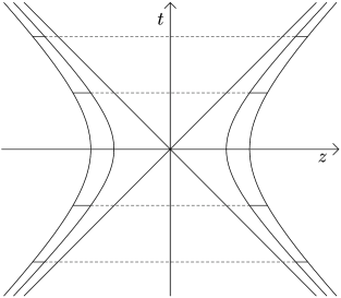
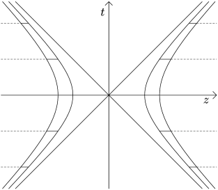
FIG. 4.: Two uniformly accelerated spinning black holes
a) connected by a spring between them,
b) with string extending from each of them to infinity.

Between the accelerated holes, i.e., for $z\in\langle-Z_{2},Z_{2}\rangle$, a nodal (string) singularity occurs (violating conditions (78), (79)) which can be understood as causing the accelerations of the holes away from each other. It is interesting to observe that there exist causality violation regions around this nodal singularity (here $g_{\varphi\varphi}<0$) which tend to be dragged along with black holes. A detailed discussion of these regions, as well as of the ergoregions of the SC-metric, will be given elsewhere.

Here, let us yet notice that, similarly to the non-rotating C-metric and, indeed, to the case of all boost-rotation symmetric spacetimes [13], we can construct SC-metrics in which the axis is regular between the holes and strings are located outside them, i.e., at $z>Z_{1}$, $z<-Z_{1}$ (see Fig 4 b). As a consequence of the field equations function $A$ in the metric (65) is constant along the axis outside the horizon, its value being different at $z>Z_{1}$, $z<-Z_{1}$ from that at $z\in\langle-Z_{2},Z_{2}\rangle$. (This can be checked by analyzing directly the expression for $A$ given by Eqs. (35), (26), (46),(50), (61)). In the above case when the nodal singularity extends between the horizons, $A=0$ at the axis for $z>Z_{1}$, $z<-Z_{1}$ (see Eq. (81)), but $A=A_{0}\not=0$ at $\rho=0$, $z\in\langle-Z_{2},Z_{2}\rangle$. Since field equations allow us to add an additive constant to $A$, we may just take $\tilde{A}(\rho,z,t)=A(\rho,z,t)-A_{0}$ which implies a regular axis between the holes but nodal singularities at $z^{2}>Z_{1}^{2}$ (see Fig. 4 b).

VI Concluding remarks

Our main result is the explicit representation (65)-(66) of the spinning C-metric as a spacetime with an axial and a boost Killing vector which are not hypersurface orthogonal. This has been achieved by first transforming the original form of the metric into the Weyl coordinates and, subsequently, by going over to coordinates adapted to boost-rotation symmetry. Simultaneously, two new “radiative” regions of the spacetime arise in which the boost Killing vector is spacelike.

Indeed, it is easy to see that under the transformation (61), (68), the Killing vector $\xi_{(\bar{t})}=\partial/\partial\bar{t}$ goes over into

$$\xi=z\frac{\partial}{\partial t}+t\frac{\partial}{\partial z}\ .$$ (86)

This is the boost Killing vector which in the coordinates adapted to the boost-rotation symmetry of the SC-metric has everywhere the same form as in flat space. Its norm is given by

$$|\xi|^{2}=-{\rm e}^{\mu}(z^{2}-t^{2})\ .$$ (87)

One can make sure that, after analytically continuing the metric (65) into the region $t^{2}>z^{2}$, the norm (87) is always positive there so that the Killing vector is spacelike.

Very recently Letelier and Oliveira [22] gave an incomplete transformation of the SC-metric into the Weyl form. However, these authors did not choose the Killing vectors and, thus, also the corresponding coordinates $\bar{t}$ and $\bar{\varphi}$ which would reflect the boost-rotational symmetry of the SC-spacetimes. In fact in contrast to our Eq. (23) relating ($\tau$, $\sigma$) to ($\bar{t},\bar{\varphi}$), they put simply $\tau\sim\bar{t}$, $\sigma\sim\bar{\varphi}$. In addition, their formula for the radial coordinate is not correct (in their last Eq. (34) the second term proportional to $(a/m)^{2}$ should not appear). This leads to an incorrect “location” of the axis in their Fig. 1 etc.

From the form (65) we have seen (cf. Eq. (72)) that the coordinates can be chosen so that the metric becomes explicitly Minkowskian at spatial infinity. We did not analyze rigorously the structure of null infinity where we expect to find a non-vanishing radiation field as it exists in the standard C-metric and, indeed, in all boost-rotation symmetric spacetimes [19]. Here we confine ourselves to giving Fig. 5 which demonstrates the radiative character of the SC-metric. In the figure the invariant proportional to $I_{3}^{\frac{1}{12}}$ and $I_{3}^{\frac{1}{6}}$, where $I_{3}$ is given by Eq. (56), is plotted at a fixed time $t=t_{0}>0$ and at different times. The radiative field has the character of a pulse, as was noticed many years ago in [14] for the special boost-rotation symmetric solutions with hypersurface orthogonal Killing vectors. It is also of interest to plot the gradient of $g_{\varphi t}\sim A$ as a function of time: here again the pulse character can be observed.

Although we did not here analyze the radiative properties of the SC-metric rigorously, it is most plausible to expect that in the situation described by Fig. 4b one can give arbitrarily strong hyperboloidal data (see [24] for a recent review and references on this approach to the initial value problem) on a hyperboloid “above the roof” $(t>|z|)$, which represent the SC-metric data and which evolve into the spacetime with smooth null infinity with a non-vanishing radiation field. No other spacetime of this type, with two Killing vectors which are not hypersurface orthogonal, is available in an explicit form. This suggests the SC-metric to become a useful, non-trivial test-bed for numerical relativity.

FIG. 5.: The plot of the curvature invariants related to $I_{3}$ in (56) at fixed $t=t_{0}>0$ (Fig. 5a). The peaks are located “above” the accelerated, rotating black holes. The gravitational radiation pulse propagates in all directions with velocity of light and decreasing amplitude as seen from Figure 5b, plotted for $\theta=\pi/2.$

Acknowledgments
V. P. enjoyed the hospitality of the Institute of Theoretical Physics of the F. Schiller-University, Jena, where part of this work was done. Helpful discussions with Alena Pravdová are gratefuly acknowledged. J. B. thanks Swiss National fonds for support and Petr Hájíček for discussions and kind hospitality at the Institute of Theoretical Physics in Berne, where this work was finished. We were supported in part by the Grant No. GACR-209/99/0261 and V. P. also by the Grant No. GACR-201/98/1452.

REFERENCES

- [1] D. Kramer, H. Stephani, M. MacCallum and E. Herlt, Exact solutions of Einstein’s Field Equations, (Cambridge University Press, 1980).
- [2] W. Kinnersley and M. Walker, Uniformly accelerating charged mass in General Relativity, Phys. Rev. D 2, 1359 (1970).
- [3] F. J. Ernst, Generalized C-metric, J. Math. Phys. 19, 1986 (1978); W. B. Bonnor, An exact solution of Einstein’s equations for two particles falling freely in an external gravitational field, Gen. Rel. Grav. 20, 607 (1988).
- [4] F. J. Ernst, Removal of the nodal singularity of the C-metric, J. Math. Phys. 17, 515 (1976).
- [5] S. W. Hawking, G. T. Horowitz and S. F. Ross, Entropy, area, and black hole pairs, Phys. Rev. D 51, 4302 (1995).
- [6] S. W. Hawking and S. F. Ross, Pair production of black holes on cosmic strings, Phys. Rev. Lett. 75, 3382 (1995).
- [7] R. B. Mann and S. F. Ross, Cosmological production of charged black hole pairs, Phys. Rev. D 52, 2254 (1995).
- [8] A. Ashtekar and T. Dray, On the existence of solutions to Einstein’s equation with non-zero Bondi-news, Comm. Phys. 79, 581 (1981).
- [9] W. B. Bonnor, The sources of the vacuum C-metric, Gen. Rel. Grav. 15, 535 (1983).
- [10] F. H. J. Cornish and W. J. Uttley, The interpretation of the C metric. The Vacuum case, Gen. Rel. Grav. 27, 439 (1995).
- [11] F. H. J. Cornish and W. J. Uttley, The interpretation of the C metric. The charged case when , Gen. Rel. Grav. 27, 735 (1995).
- [12] C. G. Wells, Extending the black hole uniqueness theorems I., gr-qc/9808044, (1998).
- [13] J. Bičák and B. G. Schmidt, Asymptotically flat radiative space-times with boost-rotation symmetry: The general structure, Phys. Rev. D 40, 1827 (1989).
- [14] J. Bičák, Gravitational radiation from uniformly accelerated particles in general relativity, Proc. Roy. Soc. A 302, 201 (1968).
- [15] J. Bičák, Radiative properties of space-times with the axial and boost symmetries, in Gravitation and Geometry, edited by W. Rindler and A. Trautman, (Bibliopolis, Naples, 1987).
- [16] J. Bičák, On exact radiative solutions representing finite sources, in Galaxies, Relativity and Axisymmetric Systems and Relativity, Essays presented to W. B. Bonnor on his 65th birthday, edited by M. A. H. MacCallum, (Cambridge University Press, Cambridge, 1985).
- [17] V. Pravda and A. Pravdová, Uniformly accelerated sources in electromagnetism and gravity, in Proceedings of the week of postgraduate students, (Charles university, Prague 1998); gr-qc/9806114 (1998).
- [18] J. Bičák, Radiative spacetimes: exact approaches, in Relativistic Gravitation and Gravitational Radiation, Proceedings of the Les Houches School of Physics, edited by J. A. Marc and J. P. Lasota, (Cambridge University Press, Cambridge, 1995).
- [19] J. Bičák, A. Pravdová, Symmetries of asymptotically flat electrovacuum spacetimes and radiation, J. Math. Phys. 39, 6011 (1998).
- [20] J. F. Plebański and M. Demiański, Rotating, charged and uniformly accelerating mass in general relativity, Annals of Phys. 98, 98 (1976).
- [21] H. Farhoosh and R. L. Zimmerman,Surfaces of infinite red-shift around a uniformly accelerating and rotating particle, Phys. Rev. D 21, 2064 (1980).
- [22] P. S. Letelier and S. R. Oliveira, On Uniformly Accelerated Black Holes, gr-qc/9809089 (1998).
- [23] W. B. Bonnor, The C-metric with , Gen. Rel. Grav. 16, 269 (1984).
- [24] H. Friedrich, Einstein’s Equations and Conformal Structure, in The Geometric Universe. Science, Geometry, and the Work of Roger Penrose, eds. S. A. Huggett et al, Oxford Univesrity Press, pp. 81-97, (1998).