Excitation of the odd parity quasi-normal modes of compact objects

Abstract

The gravitational radiation generated by a particle in a close unbounded orbit around a neutron star is computed as a means to study the importance of the $w$ modes of the neutron star. For simplicity, attention is restricted to odd parity (“axial”) modes which do not couple to the neutron star’s fluid modes. We find that for realistic neutron star models, particles in unbounded orbits only weakly excite the $w$ modes; we conjecture that this is also the case for astrophysically interesting sources of neutron star perturbations. We also find that for cases in which there is significant excitation of quadrupole $w$ modes, there is comparable excitation of higher multipole modes.

I Introduction and overview

Gravitational wave signals from perturbed black holes typically show waveforms with strong quasinormal (QN) ringing, damped oscillations at a period and damping rate characteristic of the mass and angular momentum of the hole. If the source of perturbations of the hole has no inherent time scale (as it would, for example, in the case of a particle scattered[1, 2] or plunging into the hole[3]) then QN ringing completely dominates the appearance of the waveform. Indeed, most perturbation computations show waveforms that contain only an initial transient and QN ringing. The meaning of QN ringing has been well studied in the mathematical context of perturbation calculations (Einstein’s field equations linearized about a black hole background). QN ringing, however, has also found to dominate the waveforms of black hole processes computed with numerical solutions of the full nonlinear set of Einstein’s equations[4, 5].

Unlike black holes, neutron stars have inherent time scales associated with the various possible modes of fluid motion. These fluid modes can be understood, and analyzed approximately with a semi-Newtonian approach: The excitations and frequencies of the fluid modes are analyzed with Newtonian mechanics, and the fluid motions are treated as a source in the equations of weak field general relativity. The emission of gravitational waves, in these calculations, damps the periodic fluid oscillations of Newtonian theory, but due to the weak coupling to gravitational waves these fluid QN modes are weakly damped. By contrast, the QN modes of a Schwarzschild black hole are strongly damped, with damping times of the same order as their period.

The sharp distinction between the nature of neutron star QN modes and black hole QN modes ended when studies of neutron star models by Kojima[6] and Kokkotas and Schutz[7] revealed the existence of modes that had no Newtonian counterpart. These modes, called $w$ modes (for wave modes) are general relativistic in their origin and are similar to black hole QN modes in that they are quickly damped. That $w$ modes are distinct from fluid modes is particularly clear in the existence of odd-parity $w$ modes. The quantities describing the perturbations of a spherical stellar model break up into two sets of quantities, called even and odd parity, which are not coupled by the perturbed field equations. The even parity set includes all the information about fluid motion[8]. The odd parity set includes no fluid perturbations. It describes purely relativistic modes that are perturbations only of the background geometry.

Chandrasekhar and Ferrari[9] showed that sufficiently compact homogeneous neutron star models had odd parity QN modes. Later studies [10, 11] not only confirmed these results but also showed that these odd modes exist for all degrees of stellar compactness and that the less compact the star is, the more rapidly damped are its modes. Odd parity modes of neutron stars with realistic equations of state have also been computed recently [12].

In the next few years the vibrations of neutron stars may be of more than academic interest. Neutron star processes, in various forms, are among the most plausible sources of gravitational waves that may be within the reach of detectors like LIGO, VIRGO, GEO600, TAMA300 and others. Though the $w$ modes are at frequencies above the range of high sensitivity for interferometric detectors[13], they may be interesting sources for resonant bar detectors. In 1996, Andersson and Kokkotas[14] pointed out that much work on neutron star dynamics was still being done in Newtonian theory and these studies, in principle, excluded the fundamentally relativistic $w$ modes. Andersson and Kokkotas particularly directed attention to the question that is most important about the $w$ modes: to what extent are they excited in astrophysical processes. More specifically one should ask about the relative excitation of the semi-Newtonian fluid modes and the fundamentally relativistic $w$ modes in a real astrophysical process.

The key difficulty here lies in the question of what is an acceptable model of a “real astrophysical process.” Those processes which are of greatest interest as sources of detectable waves are the oscillations of a neutron star formed in a supernova collapse or formed by the coalescence of two neutron stars as the last stage of binary inspiral. The numerical modelling of such processes with general relativistic codes is beyond near term computational capability, so “real” processes cannot be simulated. On the other hand it is not adequate to choose any convenient source of perturbations.

Andersson and Kokkotas ([14]), for instance, gave an example of the excitation of QN ringing of neutron stars by impinging gravitational waves. It is plausible that the relative excitation of $w$ modes and fluid modes for such a source is not representative of how modes would be excited by astrophysical processes. This might be said also of any source of perturbations chosen arbitrarily. The model we investigate here avoids arbitrariness by using a specific physical process. We consider a nonrotating neutron star of mass $M$ and radius $R$. An object of mass $m_{0}$ passes by the neutron star on a geodesic trajectory that is the general relativistic equivalent of a hyperbolic orbit. We make the “particle” approximation in which $m_{0}\ll M$ and the field equations are expanded in the perturbation parameter $m_{0}/M$. We study the dependence of excitation on the two parameters of the particle orbits, the particle energy and angular momentum. Neutron star models considered are limited to relativistic polytropes. In principle, our “incontrovertibly astrophysical” model would give a definitive answer to the question of the relative excitation of fluid modes and $w$ modes. But in practice the present paper gives only a partial answer and represents only a first step. Here, for simplicity, we consider only odd parity modes. The absence of coupling between odd parity perturbations and fluid motions makes the odd parity case much simpler to analyze, but it also means that there is no excitation of fluid modes with which comparisons can be made. What can be achieved is a comparison of gravitational radiation in $w$ modes, and gravitational radiation directly due to the moving particle. In this sense the present work also shows the parameter values for which $w$ mode excitation is significant. These results are of interest by themselves and probably indicate the systematics of the even parity excitations.

We present results for odd parity radiation from a range of particle trajectories and we use these results to speculate about the importance of $w$ modes in astrophysical processes. We also demonstrate that the study of the excitation of strongly damped QN modes is better carried out with waveforms than with spectra. An additional point inherent in our results is that QN ringing of higher multipoles is excited as strongly as that of quadrupole modes, though this conclusion is probably a feature only of models involving perturbations of a neutron star by a relativistic particle.

The remaining sections are organized as follows. Sec. II introduces the model problem. The wave equation describing the odd parity perturbations appear in Sec. III, the analysis of the solution with Fourier transforms is given in Sec. IV, and the method of computing solutions is presented in Sec. V. Results are presented and discussed in Sec. VI, and conclusions are briefly summarized in Sec. VII. Some relevant details of particle orbits in the Schwarzschild geometry are given in an appendix. Throughout the paper we use geometric units $G=c=1$ and metric signature $(+,-,-,-)$.

As this paper was in preparation we learned of two works dealing with excitation of QN modes of a neutron star: a paper by Tominaga et al.[15] on substantially the same problem investigated here, and a paper by Ferrari et al[16] which considers the excitation of the even parity modes. Among the differences between these works and the present paper are an emphasis on waveforms rather than spectra as a mean to detecting excitation of QN modes, the study of high energy orbits and of odd modes of neutron stars of radius greater than $3M$.

II The model: Perturbation of a static star by a particle moving in a scattered geodesic

In our model of gravitational interaction, we start with a static and spherically symmetric spacetime background metric

$$ds^{2}=e^{\nu(r)}dt^{2}-e^{\lambda(r)}dr^{2}-r^{2}[d\theta^{2}+\sin^{2}\theta d\varphi^{2}]$$ (1)

describing both the interior and exterior of a star of ideal fluid of mass M and radius $r=R$. The stress energy of the fluid is

$$T_{\alpha\beta}=(\rho+p)u_{\alpha}u_{\beta}-pg_{\alpha\beta}$$ (2)

where $\rho$ is the mass-energy density and $p=p(\rho)$ is the pressure. The mass function $m(r)$ is defined by $e^{-\lambda(r)}=1-2m(r)/r$, and the structure of the stellar interior is found by solving the hydrostatic equilibrium equations of general relativity

$$\frac{dm}{dr}=4\pi r^{2}\rho$$ (3)

$$\frac{d\nu}{dr}=-\frac{2}{\rho+p}\frac{dp}{dr}$$ (4)

$$\frac{dp}{dr}=-\frac{(\rho+p)[m(r)+4\pi r^{3}p]}{r[r-2m(r)]}\ .$$ (5)

We limit considerations here to stellar interiors that are relativistic polytropes[17]. The polytropic equation of state has the simple algebraic form

$$p/p_{0}=(\rho/\rho_{0})^{1+1/n}\ ,$$ (6)

A particular model is specified by fixing the polytropic index, $n$, (in general not an integer) and the central density and pressure $\rho_{0},p_{0}$. With these fixed one can integrate to the surface (i.e, the radius at which $p=0$) and find the value of the star’s radius $R$, and mass $M=m(R)$. The ratio $M/R$ is an indication of “how relativistic” the stellar model is. A particularly simple class of polytropics is the $n=0$ constant density stars. For these models the metric coefficients are found to have the closed forms

$$e^{\nu(r)}=\left[\frac{3}{2}\sqrt{1-\frac{2M}{R}}-\frac{1}{2}\sqrt{1-\frac{2Mr^{2}}{R^{3}}}\right]^{2}\hskip 20.0ptr\leq R$$ (7)

$$e^{-\lambda(r)}=\left(1-{2Mr^{2}}/{R^{3}}\right)\hskip 20.0ptr\leq R\ .$$ (8)

It is evident in (7) that $e^{\nu(0)}$ vanishes for $M/R=4/9$. This well known limit to how relativistic a homogeneous model can be corresponds to infinite central pressure. Outside the star, the metric functions take their familiar Schwarzschild form,

$$e^{-\lambda(r)}=e^{\nu(r)}=1-(2M/r)\hskip 10.0ptr\geq R,$$ (9)

A point particle of mass $m_{0}\ll M$, starting from infinity, passes close to the star (but never enters it), is scattered and proceeds out to infinity. We treat the particle as a perturbation of the spacetime inside and outside the star, and we analyze the perturbations only to first order in $m_{0}/M$. The radiation reaction is second order in this perturbation parameter, so we can ignore it and assume that the particle moves along a scattered geodesic of the unperturbed spacetime exterior to the star, i.e. of Schwarzschild spacetime. The metric of the perturbed spacetime can be written as

$$g_{\alpha\beta}=g^{(0)}_{\alpha\beta}+h_{\alpha\beta}\ ,$$ (10)

where the “(0)” index here and below denotes the background solution. The Einstein equations to first order in perturbations are

$$\delta R_{\alpha\beta}=8\pi[\delta T_{\alpha\beta}-\frac{1}{2}\delta Tg^{(0)}_{\alpha\beta}-\frac{1}{2}T^{(0)}h_{\alpha\beta}]\ .$$ (11)

where $T^{(0)}=\rho-3p$. The perturbed stress energy has two contributions. One contribution is that of the fluid perturbations, a contribution we ignore for reasons given below. The other contribution is the stress energy of the scattered particle. We take the particle to be moving in the ($\theta=\pi/2$) equatorial plane on a timelike geodesic in which its position as a function of coordinate time is given by $z^{\alpha}(t)$. With this notation the particle stress energy in the coordinates (1) is given by

$$\delta T^{\alpha\beta,particle}=m_{0}\frac{dt}{d\tau}\frac{\delta[r-R(t)]}{r^{2}}\delta[\cos\theta]\delta[\varphi-\varphi(t)]\frac{dz^{\alpha}}{dt}\frac{dz^{\beta}}{dt}\ .$$ (12)

Here $R(t)$ and $\phi(t)$ are respectively the Schwarzschild radial and azimuthal coordinates, as functions of Schwarzschild coordinate time, for the particle orbit.

III The wave equation governing odd parity perturbations

A decomposition of perturbation tensors in tensor spherical harmonics (see [18]) leads to a split of (11) into two sets of decoupled equations [19] called even and odd parity. Fluid perturbations are purely even parity and couple only to even parity spacetime perturbations. Since we consider here only the odd parity (sometimes also called axial) perturbations, our analysis involves only the stress energy perturbations of the particle itself, as given in (12)

We adopt the notation of Regge and Wheeler[20] and of Moncrief[21]. In this notation the only nonvanishing odd parity metric perturbations, for a particular $l,m$ multipole, are

$$h_{t\theta}=-h_{0}^{lm}(r,t)(\partial/\sin{\theta}\partial\varphi)Y_{lm}\ \ \ \ h_{t\varphi}=h_{0}^{lm}(r,t)(\sin{\theta}\partial/\partial\theta)Y_{lm}$$ (13)

$$h_{r\theta}=-h_{1}^{lm}(r,t)(\partial/\sin{\theta}\partial\varphi)Y_{lm}\ \ \ h_{r\varphi}=h_{1}^{lm}(r,t)(\sin{\theta}\partial/\partial\theta)Y_{lm}$$ (14)

$$h_{\theta\theta}=-h_{\varphi\varphi}/\sin^{2}{\theta}=h_{2}^{lm}(r,t)(\partial^{2}/\sin{\theta}\partial\theta\partial\varphi-\cos{\theta}\partial/\sin^{2}{\theta}\partial\varphi)Y_{lm}$$ (15)

$$h_{\theta\varphi}=\textstyle{\frac{1}{2}}h_{2}^{lm}(r,t)(\partial^{2}/\sin{\theta}\partial\varphi\partial\varphi+\cos{\theta}\partial/\partial\theta-\sin{\theta}\partial^{2}/\partial\theta\partial\theta)Y_{lm}\ .$$ (16)

For simplicity, for now we make the Regge-Wheeler[20] gauge choice, which for odd-parity means that we choose $h_{2}^{lm}=0$. By taking a combination of the odd parity perturbed vacuum Einstein equations, Regge and Wheeler[20] showed that $Q_{lm}(r,t)$ defined by

$$Q_{lm}(r,t)\equiv e^{[\nu(r)-\lambda(r)]/2}\frac{h_{1}^{lm}(r,t)}{r}$$ (17)

satisfies a simple homogeneous wave equation. The same combination of odd parity equations with stress energy perturbations[18] results in a wave equation with a source term, of the form

$$\frac{\partial^{2}Q_{lm}}{\partial t^{2}}-\frac{\partial^{2}Q_{lm}}{\partial r^{*2}}+\left\{l(l+1)-\frac{6m(r)}{r}+4\pi r^{2}[\rho(r)-p(r)]\right\}\frac{Q_{lm}}{r^{2}}e^{\nu(r)}={\cal S}_{lm}(r,t)\ .$$ (18)

Here $r^{*}$ is the usual tortoise coordinate

$$\frac{dr}{dr^{*}}=e^{[\nu(r)-\lambda(r)]/2}\ ,$$ (19)

which, in the vacuum outside the star, can be written as

$$r^{*}=r+2M\log[r/2M-1]+{\rm const}\ .$$ (20)

The source term, ${\cal S}_{lm}(r,t)$, is constructed from the stress energy (12) of the particle. For a particle of mass $m_{0}$, moving in the equatorial ($\theta=\pi/2$) plane, with energy per mass $E$, and angular momentum per mass $L$, the $l,m$ multipole of the source term has the form

$${\cal S}_{lm}(r,t)=\left(1-\frac{2M}{r}\right)\left(1-\frac{3M}{r}\right)\frac{2{\cal D}_{lm}}{r^{2}}-\frac{{\cal D}_{lm,r}}{r}\left(1-\frac{2M}{r}\right)^{2}+\frac{{\cal C}_{lm}}{r}\left(1-\frac{2M}{r}\right)$$ (21)

where

$${\cal D}_{lm}=D_{lm}\delta[r-R(t)]\hskip 72.26999pt{\cal C}_{lm}=C_{lm}\delta[r-R(t)]$$ (22)

with

$${D}_{lm}=\frac{16\pi imm_{0}}{(l-1)l(l+1)(l+2)}\frac{L^{2}}{Er^{2}}\frac{\partial Y^{*}_{lm}}{\partial\theta}[\pi/2,\varphi(t)]$$ (23)

$${C}_{lm}=-\frac{16\pi m_{0}}{l(l+1)}\frac{dR}{dt}\frac{L}{r^{2}}\frac{\partial Y^{*}_{lm}}{\partial\theta}[\pi/2,\varphi(t)]\ .$$ (24)

In the Schwarzschild spacetime outside the star (18) is the well known Regge-Wheeler equation[20].

IV Fourier transform of the wave equation

The equation in (18) could be solved directly with a finite difference representation of the 1+1 partial differential equation. Our Cauchy data for this equation, however, correspond to the particle “starting” at infinity with no incoming radiation. These starting conditions are most simply handled with a Fourier representation of the problem, so we write $Q_{lm}(r,t)$ as a Fourier integral

$$Q_{lm}(r,t)=\frac{1}{2\pi}\int_{-\infty}^{\infty}e^{-i\omega t}\widetilde{Q}_{lm}(r,\omega)d\omega$$ (25)

and transform (18) into a second order ODE for $\widetilde{Q}_{lm}(r,\omega)$,

$$\frac{d^{2}\widetilde{Q}_{lm}}{dr^{*2}}+\left\{\omega^{2}-\left[\frac{l(l+1)}{r^{2}}-\frac{6m(r)}{r^{3}}+4\pi(\rho(r)-p(r))\right]e^{\nu(r)}\right\}\widetilde{Q}_{lm}(r,\omega)=-\widetilde{S}_{lm}(r,\omega)$$ (26)

where

$$\widetilde{S}_{lm}(r,\omega)=\int_{-\infty}^{\infty}S_{lm}(r,t)e^{i\omega t}dt$$ (27)

is the Fourier transform of the source term.

At infinity, the wave will be purely outgoing so that

$$\begin{array}[]{cc}\widetilde{Q}_{lm}(r,\omega)\rightarrow A_{lm}(\omega)e^{i\omega r^{*}},&r^{*}\rightarrow\infty\ .\end{array}$$ (28)

It follows that at infinity, ${Q}_{lm}$ is a function of retarded time $u\equiv t-r^{*}$ given by

$$Q_{lm}(u\equiv t-r^{*})=\frac{1}{2\pi}\int_{-\infty}^{\infty}A_{lm}(\omega)e^{-i\omega u}d\omega\ .$$ (29)

It is useful to note that the definition of $Q_{lm}$ in terms of multipole components of the real quantities $h_{ij}$, and the property $Y_{lm}^{*}=(-1)^{m}Y_{l,-m}$ of the spherical harmonics, require

$$A_{lm}(\omega)=(-1)^{m}A^{*}_{l,-m}(-\omega)\ .$$ (30)

The gravitational (odd parity part) power, radiated to infinity is given by [22]

$$P=\frac{1}{16\pi}\sum_{l=2}^{\infty}\sum_{m=-l}^{l}\frac{(l+2)!}{(l-2)!}|Q_{lm}(u)|^{2}\ .$$ (31)

Using (29) and Parseval’s theorem we obtain the odd parity part of the energy spectrum

$$\frac{dE}{d\omega}=\frac{1}{16\pi^{2}}\sum_{l=2}^{\infty}\sum_{m=-l}^{l}\frac{(l+2)!}{(l-2)!}|A_{lm}(\omega)|^{2}\ .$$ (32)

From the wavefunction $Q_{lm}(u)$ we can construct the multipoles of the metric perturbations. Of particular interest are the transverse strains of gravitational waves. In an asymptotically flat gauge these are the perturbations $h_{\theta\theta},h_{\phi\phi},h_{\theta\phi}$. To compute the relationship between $Q_{lm}$ and perturbations in an asymptotically flat gauge it is useful to note that the quantity

$$Q^{{\rm Monc}}_{lm}=\frac{1}{r}\left(1-\frac{2M}{r}\right)\left(h_{1}^{lm}+\frac{1}{2}\left[\frac{\partial h_{2}^{lm}}{\partial r}-\frac{2}{r}h_{2}^{lm}\right]\right)$$ (33)

has been shown by Moncrief[21] to be a gauge invariant combination of odd-parity metric perturbations in the Schwarzschild background. In the stellar exterior, in the Regge-Wheeler gauge, the perturbation $Q^{{\rm Monc}}_{lm}$ agrees with our wave function $Q_{lm}$. It follows that $Q_{lm}$ is identical to $Q^{{\rm Monc}}_{lm}$ in the stellar exterior, and that in the exterior we can take (33) to be the definition of (17) in an arbitrary gauge. Since the right hand side of (33) is gauge invariant, we can evaluate the relationship between $Q_{lm}$ and the metric perturbations in an asymptotically flat gauge, at large radius. In this case, the expression for $Q_{lm}$ in (33) reduces to

$$Q_{lm}=\frac{1}{2}\frac{\partial h_{2}^{lm}}{\partial r}+{\cal O}(r^{-2})=-\frac{1}{2}\dot{h}_{2,lm}+{\cal O}(r^{-2})\ .$$ (34)

Here the dot over ${h}_{2}^{lm}$ indicates the derivative with respect to retarded time $u$. The last equality in (34) follows from the fact that ${h}^{lm}_{2}$ is a function of $u$ aside from corrections higher order in $1/r$. From (34) we have $\dot{h}_{2}^{lm}$ and hence, with (13) we have, for example,

$$\dot{h}_{\theta\theta}=\dot{h}_{2}^{lm}(r,t)(\partial^{2}/\sin{\theta}\partial\theta\partial\varphi-\cos{\theta}\partial/\sin^{2}{\theta}\partial\varphi)Y_{lm}\ .$$ (35)

But this multipole component is complex. To get meaningful physical quantities we need to sum multipole components with $\pm m$. In doing this it is useful to define:

$$F_{1}^{l,m} = \frac{1}{\sin\theta}\left[\frac{\partial}{\partial\theta}-\cot\theta\right]Y_{lm}(\theta,\varphi)$$ (36)

$$F_{2}^{l,m} = \frac{1}{2}\left[-\frac{m^{2}}{\sin^{2}\theta}+\cos\theta\frac{\partial}{\partial\theta}-\sin\theta\frac{\partial^{2}}{\partial\theta^{2}}\right]Y_{lm}(\theta,\varphi)\ .$$ (37)

For a given pair of multipole modes $l,m$ and $l,-m$ we can then construct real functions

$$-\dot{h}_{\varphi\varphi}^{l,\Sigma m}/\sin^{2}{\theta}=\dot{h}_{\theta\theta}^{l,\Sigma m}\equiv\dot{h}_{\theta\theta}^{l,m}+\dot{h}_{\theta\theta}^{l,-m} = 4|m|r\left[{\rm Re}\left(Q^{lm}\right)\sin{|m|\varphi}+{\rm Im}\left(Q^{lm}\right)\cos{|m|\varphi}\right]F_{1}^{l,|m|}$$ (38)

$$\dot{h}_{\theta\varphi}^{l,\Sigma m}\equiv\dot{h}_{\theta\varphi}^{l,m}+\dot{h}_{\theta\varphi}^{l,-m} = 4r\left[-{\rm Re}\left(Q^{lm}\right)\cos{|m|\varphi}+{\rm Im}\left(Q^{lm}\right)\sin{|m|\varphi}\right]F_{2}^{l,|m|}\ .$$ (39)

V Computational implementation

A Solution for $A_{lm}(\omega)$

If the background spacetime is due to a star, equation (26) is to be solved for the boundary conditions of a regular solution at the center of the star and outgoing waves at spatial infinity: $Q_{lm}(r,\omega)\rightarrow r^{l+1}$ for $r\rightarrow 0$ and $Q_{lm}(r,\omega)\rightarrow e^{i\omega r^{*}}$ for $r\rightarrow\infty$. The Green function solution is found in the usual way. We define $y^{\rm reg}_{l}(r,\omega)$ and $y^{\rm out}_{l}(r,\omega)$ as the homogeneous solutions of (26) with asymptotic forms

$$\begin{array}[]{cc}y^{\rm reg}_{l}(r,\omega)\rightarrow r^{l+1},&r\rightarrow 0\\ y^{\rm out}_{l}(r,\omega)\rightarrow e^{i\omega r^{*}},&r\rightarrow\infty\ .\end{array}$$ (40)

We then define the Wronskian of these two homogeneous solutions, an $r$ independent constant, to be

$$W_{l}(\omega)=y^{\rm reg}_{l}\frac{dy^{\rm out}_{l}}{dr^{*}}-y^{\rm out}_{l}\frac{dy^{\rm reg}_{l}}{dr^{*}}\ .$$ (41)

With the above definitions, the Green function solution is

$$\widetilde{Q}_{lm}(r,\omega)=-\frac{1}{W_{l}(\omega)}\left[y^{\rm out}(r^{*},\omega)\int_{r^{*}_{t}}^{r^{*}}\widetilde{S}_{lm}(r^{{}^{\prime}*},\omega)y^{\rm reg}(r^{*^{\prime}},\omega)dr^{*^{\prime}}\right.$$ (42)

$$\left.+y^{\rm reg}(r^{*},\omega)\int_{r^{*}}^{\infty}\widetilde{S}_{lm}(r^{*^{\prime}},\omega)y^{\rm out}(r^{*^{\prime}},\omega)dr^{*^{\prime}}\right]\ ,$$ (43)

where the lower limit in the first integral, $r^{*}_{t}\equiv r^{*}(r_{t})$, denotes the value of $r^{*}$ at the minimum radius (turning point) of the scattered orbit. In the limit of large $r$, a comparison of (28) with (43) gives us

$$A_{lm}(\omega)=-\frac{1}{W_{l}(\omega)}\int_{r^{*}(0)}^{\infty}\widetilde{S}_{lm}(r^{*},\omega)y^{\rm reg}(r^{*},\omega)dr^{*}$$ (44)

With the notation for ${\cal C}_{lm},{\cal D}_{lm}$ in (21) – (22) the expression for $\widetilde{S}_{lm}(r,\omega)$ takes the form

$$\widetilde{S}_{lm}(r,\omega)=\int_{-\infty}^{\infty}dte^{i\omega t}\left\{\left[\left(1-\frac{2M}{r}\right)\left(1-\frac{3M}{r}\right)\frac{2D_{lm}}{r^{2}}-\frac{D_{lm,r}}{r}\left(1-\frac{2M}{r}\right)^{2}\right.\right.$$ (45)

$$\left.\left.+\frac{C_{lm}}{r}\left(1-\frac{2M}{r}\right)\right]\delta[r-R(t)]-\frac{D_{lm}}{r}\left(1-\frac{2M}{r}\right)^{2}\frac{d\delta[r-R(t)]}{dr}\right\}\ .$$ (46)

Substituting this expression into (44), and using the properties of the $\delta$ function, we get

$$A_{lm}(\omega)=-\frac{1}{W_{l}(\omega)}\left\{\int_{-\infty}^{\infty}dte^{i\omega t}y^{\rm reg}[R,\omega]\left[\left(1-\frac{2M}{R}\right)\frac{D_{lm}}{R^{2}}+\frac{C_{lm}}{R}\right]\right.$$ (47)

$$\left.+\int_{-\infty}^{\infty}dte^{i\omega t}\frac{dy^{\rm reg}}{dr}\frac{D_{lm}}{R}\left(1-\frac{2M}{R}\right)\right\}\ .$$ (48)

For the geodesics considered in this work (scattered geodesics, see appendix A), we can distinguish two phases of the motion: In the first, the particle comes from infinity and moves towards the star until reaching the turning point; it then returns to infinity in the second region. If we choose the origin of coordinate time and angle $\varphi$ at the turning point, then for any time $t=-\bar{t}$ and angle $\varphi=-\bar{\varphi}$ in the first, inward, phase of the motion, there is a corresponding point $t=\bar{t},\varphi=\bar{\varphi}$ during the second, outward, phase. The symmetry of the inward and outward motions allows us to write the amplitude as an integral only over positive time,

$$A_{lm}(\omega)=-\frac{2i}{W_{l}(\omega)}\left\{\int_{0}^{\infty}y^{\rm reg}(R,\omega)dt\left[\left(1-\frac{2M}{R}\right)\frac{|D_{lm}|}{R^{2}}\cos(\omega t-m\varphi(t))+\frac{|C_{lm}|}{R}\sin(\omega t-m\varphi(t))\right]\right.$$ (49)

$$\left.+\int_{0}^{\infty}dt\frac{dy^{\rm reg}}{dt}\frac{|D_{lm}|}{r}\left(1-\frac{2M}{R}\right)\cos(\omega t-m\varphi(t))\right\}\ ,$$ (50)

where $|D_{lm}|=-iD_{lm}{exp(im\varphi)},|C_{lm}|=C_{lm}exp(im\varphi)$ with $D_{lm},C_{lm}$ given by (23-24). Once the quantities $A_{lm}(\omega)$ are computed, the waveform follows from (38) and the energy spectrum from (32).

If the particle moves outside a spherically symmetric black hole, not a star, then the amplitude can be obtained from (50) with only two changes. The ingoing solution $y^{ing}$ (see [23]), of the Regge-Wheeler equation must be substituted for $y^{\rm reg}$ in the integral in (50), and the Wronskian defined in (41) must be replaced by

$$W_{l}(\omega)=y^{\rm ing}_{l}\frac{dy^{\rm out}_{l}}{dr^{*}}-y^{\rm out}_{l}\frac{dy^{\rm ing}_{l}}{dr^{*}}\ .$$ (51)

B Numerical method

The first step in the determination of the amplitude and waveform is the computation of the regular homogeneous solution of the equation (26). The numerical problem can be divided in two parts: Integration of (26) from the center of the star to its surface. And then from the surface to the point (outside the star) where we want to compute $y^{\rm reg}(r)$. Due to the presence of the centrifugal potential, which diverges at the center of the star, it is convenient to introduce, inside the star, the new function $Z_{l}$, through

$$y^{\rm reg}_{l}=r^{l+1}Z_{l}(r)$$ (52)

and instead of (26), integrate

$$\frac{d^{2}Z_{l}}{dr^{2}}+\left\{\frac{2(l+1)}{r}+e^{\lambda(r)}\left[\frac{2m(r)}{r^{2}}+4\pi r(p-\rho)\right]\right\}\frac{dZ_{l}}{dr}+$$ (53)

$$\left[\omega^{2}e^{-\nu(r)}+\frac{(8-2l^{2})m(r)}{r^{3}}+4\pi[p(r)-\rho(r)](l+2)\right]e^{\lambda(r)}Z_{l}=0$$ (54)

from a point $r_{0}$, near the center of the star, using the starting conditions

$$Z_{l}(r_{0})=1+\frac{r^{2}_{0}}{2l+3}\left\{[(2l+3)l-2]\frac{2\pi}{3}\rho_{0}-\frac{\omega^{2}e^{-\nu_{0}}}{2}-2\pi(l+2)p_{0}\right\}$$ (55)

$$\frac{dZ_{l}}{dr}(r_{0})=\frac{2r_{0}}{2l+3}\left\{[(2l+3)l-2]\frac{2\pi}{3}\rho_{0}-\frac{\omega^{2}e^{-\nu_{0}}}{2}-2\pi(l+2)p_{0}\right\},$$ (56)

until reaching the surface of the star, $r=R$ where we switch back to $y^{\rm reg}_{l}$ and integrate

$$\frac{d^{2}y^{\rm reg}_{l}}{dr^{2}}+\frac{1}{1-2M/r}\frac{2M}{r^{2}}\frac{dy^{\rm reg}_{l}}{dr}+\frac{1}{(1-2M/r)^{2}}\left\{\omega^{2}-\left(1-\frac{2M}{r}\right)\left[\frac{l(l+1)}{r^{2}}-\frac{6M}{r^{3}}\right]\right\}y^{\rm reg}_{l}=0$$ (57)

from $r=R$, with the starting conditions,

$$y^{\rm reg}_{l}(R)=R^{l+1}Z_{l}(R)$$ (58)

$$\frac{dy^{\rm reg}_{l}}{dr}=R^{l+1}\frac{dZ_{l}}{dr}(R)+(l+1)R^{l}Z_{l}(R)$$ (59)

until the desired point $r$.

Both (54) and (57) follow from a rewriting of (26) in terms of the variable $r$. This avoids the numerically time consuming task of finding $r(r^{*})$.

If the unperturbed spacetime is a Schwarzschild black hole instead of a star, then instead of $y^{\rm reg}_{l}$ we need to find $y^{\rm ing}_{l}$, the purely ingoing (at the horizon) homogeneous solution of (26). This is done by substituting $y^{\rm reg}_{l}$ by $y^{\rm ing}_{l}$ in (57) and integrating from a large negative value of $r^{*}$ with the “initial” condition $y^{\rm ing}_{l}\sim e^{-i\omega r^{*}}$.

The computation of the Wronskian in (41) or (51) is now straightforward. We simply compute $y^{\rm reg}_{l}$ (or $y^{\rm ing}_{l}$) at large values of $r$ and use the asymptotic form of $y^{\rm out}_{l}$ at large r

$$y^{\rm out}_{l}(r\rightarrow\infty)\sim e^{i\omega r^{*}}\left[1-\frac{l(l+1)}{2i\omega r}\right]$$ (60)

to find the Wronskian by definition.

One point worth of mention is that since

$$\frac{\partial Y^{*}_{lm}}{\partial\theta}[\pi/2,0]=-\sqrt{\frac{2l+1}{4\pi}\frac{(l-m)!}{(l+m)!}}\frac{2^{m+1}}{\sqrt{\pi}}\frac{\Gamma[1+(l+m)/2]}{\Gamma[1/2+(l-m)/2]}\sin[\frac{\pi}{2}(l+m)],$$ (61)

where $\Gamma$ denotes the Gamma function, $A_{lm}\neq 0$, for a given $l$, only when $m=-l+1,-l+3,...,l-1$. Thus for $l=2$ only $A_{21},A_{2-1}$ are non zero and for $l=3$ only $A_{30},A_{32},A_{3-2}$ are non zero.

A consequence is that if, as we will do in the next section, we restrict attention to the waveform seen by an observer in the plane where the particle moves, then $\dot{h}^{l,\sum m}_{\theta\varphi}=0$ in (38) and the waveform will be polarized in the direction $\varphi,\varphi$.

VI Numerical Results and Discussion

Our presentation of results starts with gravitational radiation in the quadrupole ($l=2$) and octupole ($l=3$) modes, for a particle moving around a nonrotating black hole (see also [1],[2]). Though our main interest here is neutron star $w$ modes, it will be useful to establish the black hole results for comparison. The case of a black hole will also be helpful in clarifying several issues relevant to the neutron star case. An additional motivation for the presentation of these results is to demonstrate that in cases in which $l=2$ QN ringing is important, the $l=3$ ringing tends to be comparable, both for black holes and neutron stars.

It will be useful to understand the aspects of the emerging radiation that are associated with the motion of the particle, and those that may be ascribed to the influence of the background spacetime. (There is, of course, no fully satisfactory way of making such a distinction.) If the particle were in a periodic orbit with frequency $\Omega$, its gravitational perturbations would be functions of $\varphi-\Omega t$, and $l,m$ multipoles would have time dependence only at frequency $m\Omega$. For the scattering orbits one would expect that the characteristic peak of the spectrum would follow an approximate form of this rule with the particle’s angular velocity $d\varphi/dt$ at the turning point $r_{t}$ taking the place of $\Omega$. In the discussion below we will use the expression “particle frequency” to denote this nonrelativistically expected peak frequency $m\,d\varphi/dt$. Note that, as discussed above, an orbit in the equatorial plane is a source only for multipoles with $m=l-1,l-3,\cdots,-l+1$. Thus, $m$ will be 1 for quadrupole radiation and 2 for octupole.

Figures 1 a and b show $l=2$ and $l=3$ spectra and waveforms for orbits with particle energy parameter $E$ (energy per particle mass) of 2. For the particle motion in Fig. 1 the angular frequency $d\varphi/dt$ of the particle at the turning point is $0.18/M$ so that the particle frequency is $0.18/M$ for quadrupole radiation and $0.36/M$ for octupole. The waveform in Fig. 1b shows more specifically that QN ringing is an important part of the waveform.

The locations of the real parts of the least damped QN modes, $\omega M=.374$ for $l=2$ and $\omega M=.599$ for $l=3$, are indicated with arrows in Fig. 1 a. The analogy with normal mode systems would suggest that the extent to which particle motion stimulates QN ringing increases the closer the characteristic particle frequency is to the QN frequency. In the case of Fig. 1 a the (odd parity $m=2$) particle frequency for $l=3$ case is twice that for the (odd parity $m=1$) $l=2$ case, and the $l=3$ QN frequency is around 60% higher than the $l=2$ QN frequency. Both particle frequencies are roughly equal in the suitability for exciting the respective QN modes, and the plots show that QN ringing seems to be of roughly equal importance for $l=2$ and $l=3$.

The presence of QN radiation is fairly clear in the waveform, shown in Fig. 1 b. This figure shows the gravitational radiation, a mixture of effects of particle radiation and QN ringing. It does not tell us what fraction of the radiated energy is in QN ringing, but that question probably cannot be given a clear formulation in any case[24]. As an indicator of the importance of QN ringing, a plot of the waveform has a clear advantage, but it also has a disadvantage. To show the waveform 38 we must choose a direction in the $\theta,\varphi$ 2-sphere. The curve in Fig. 1 b corresponds to the equatorial plane ($\theta=\pi/2$) and to $\varphi=\pi/2$. The appearance of the waveform in other directions will differ. As an indication of the complexity of the waveform dependence on direction, a quadrupole waveform in the equatorial plane is shown in Fig. 2. The radiation is that for a particle with $E=2$ and $L=10M$ moving in the field of a constant density star with $R=3.125M$. The waveform amplitude, ${\rm Re}(Q_{21})\sin\varphi+$ ${\rm Im}(Q_{21})\cos\varphi$, is plotted above a cartesian plane with $x\equiv r^{*}\cos\varphi$, $y\equiv r^{*}\sin\varphi$. The direction of the symmetry axis of the particle orbit is the straight line $y=0$ in the figure. Some symmetries of the radiation pattern can be seen in Fig. 2. Since the radiation is $m=1$ radiation, the amplitude at a given time (i.e. , at a given value of $r^{*}$) must be antisymmetric under $\varphi\rightarrow\varphi+\pi$. At each radius in Fig. 2, then, the variation in amplitude must have two nodes. It is interesting to note that the particle trajectory is a symmetric one (it has a line of bilateral symmetry) but the radiation pattern is not symmetric since there is a delay in time between the radiation given off by the initial and final portions of the particle trajectory.

Despite this element of angular choice, the waveforms are the preferred tools for assessing the excitation of QN ringing in cases, like that of Fig. 1, for which the QN mode “resonance” is broad. In the case of narrow resonances, such as the QN modes for ultracompact (and probably unrealistic) stellar models, the spectrum itself is the better indicator. This is clearly shown in Fig. 3 in which results are given for a constant density stellar model with $R=2.33M$, very close to the lowest allowed limit $R/M=9/4$. For this stellar model the four lowest damped $l=2$ QN modes are $\omega_{I}M=0.281+i0.00014$, $\omega_{II}M=0.372+i0.0048$, $\omega_{III}M=0.458+i0.025$ and $\omega_{IV}M=0.554+i0.049$. The results are given for $l=2$ radiation from a particle with $E=2,L=10M$. Plots are presented for the waveform, in the direction $\theta=\pi/2,\varphi=0$, and for the energy spectrum. It is apparent in the latter that the first two QN modes of the star are excited and there are hints that all the first four might also be. The picture given by the waveform is rather more confusing due to the simultaneous presence of the two modes $\omega_{I}$ and $\omega_{II}$ with very small damping. The most obvious feature of the waveform, in fact is the beat frequency between these two almost periodic modes. For the case of this stellar model with several competing QN frequencies, and with sharp QN resonances, the nature of QN excitation is more clearly shown by the spectrum than the waveform. A second spectrum in Fig. 3, for a particle with a smaller energy of $E=1.2$ shows that the spectrum is equally useful for a particle orbit that is not highly relativistic. An interesting feature of the spectra is that the $w$ modes appear as narrow spikes at the QN resonances. These spikes contain little energy, but they appear at the high frequency boundaries of broad spectral peaks very distinct from the particle radiation spectrum.

The very sharp QN resonances appear to be unique to ultracompact stellar models. Since we will be concerned here, for the most part, with more-or-less realistic models, with broad QN resonances, we will rely on waveform pictures in our study of excitation of QN ringing. We will choose to clarify the presence of QN ringing in these waveforms by displaying them as linear-log plots of the magnitude of the waveform. In such plots QN ringing appears as a distinct sequence of bumps whose peaks lie on a straight line. The spacing of the bumps gives the real part of the QN frequency and the slope of the line gives the imaginary part. The distinctive nature of QN ringing in such a plot is shown in Fig. 4. The waveform is shown in (a) and (b) respectively for the $l=2$ and $l=3$ multipoles of the orbit used for Fig. 1. In (b) the waveform is also shown for an orbit with $E=3.7$, $L=20M$, and a turning point at $r_{t}=3.767501M$. The pattern of bumps in part (b) has the same spacing and slope for both orbits, confirming the fact that the QN frequency is independent of the source. The higher oscillation rate and roughly equal damping for $l=3$ in comparison with $l=2$ is evident in the patterns in (a) and (b). The QN frequencies found from these linear-log plots are $\omega M=0.374+i0.090$ for $l=2$, and $\omega M=0.600+i0.093$ for $l=3$. These are in excellent agreement with the known values $\omega M=0.3736+i0.089$ for $l=2$, and $\omega M=0.5994+i0.0927$ for $l=3$. The combination of parameters ($E=3.7,L=20M$) for the comparison waveform in Fig. 4 b was chosen because it gives excitation of QN ringing comparable to that for $E=2,L=10M$. It is worth noting that the particle frequency $2d\varphi/dt$ is almost identical for the two sets of parameters.

In Fig. 5 we present linear-log waveforms for a constant density stellar model with $R/M=2.5$, an ultracompact stellar model that is astrophysically implausible, but that is useful as an illustration. The real part of the $l=2,m=1$ waveforms are shown for particle orbits with the relatively low energy $E=1.2$, and for a higher energy $E=2$. For each energy one model is a low $L$ orbit with a small turning point $r_{t}$, and the other model has large $L$ and large $r_{t}$. In each case the large $r_{t}$ orbit gives far weaker QN ringing than does the small $r_{t}$ orbit. The long sequence of well defined bumps for the small $r_{t}$ models in Fig. 5 allow a graphical determination of the least damped $l=2$ QN frequency $\omega M=0.4123+i0.02199$, to accuracy of better than 1%.

Results for orbits around a constant density model with $R/M=3.125$ are shown in Fig. 6, for two different values of $L$ at each of two different values of $E$. For this model the least damped $l=2$ QN mode has a frequency $\omega M=0.455+i0.1386$ with a real part slightly higher than for a black hole ( $0.39M^{-1}$) or an ultracompact $R/M=2.5$ model ($0.41M^{-1}$). More important, the imaginary part of the QN frequency is large, around 50% larger than for a black hole and more than 6 times that for the ultracompact stellar model. The strong ringing part observed for the two smaller angular momenta can be approximated with precision better than 1% by the lowest damped QN mode.

The patterns and trends in Figs. 5 and 6 continue in Fig. 7, in which waveforms are given for constant density models with $R/M=4$, a value close to the typical radius of a neutron star. In this case the least damped $l=2$ QN mode has frequency $\omega M=0.401+i0.209$, so the QN resonance is extremely broad. A consequence is that the pattern of QN bumps is less clear in the linear-log waveforms. For the low $L$, high particle frequency orbits, there is evidence of excitation of the lowest damped QN mode for both energies, but none for the high values of L. The energy spectra for these models are presented in Fig. 8. For homogeneous stars with $R/M>4$, the damping of QN modes will be even stronger than in Fig. 7, and QN ringing will be even less apparent in the waveform.

The results presented in the previous figures are not sensitively dependent on the assumption of a homogeneous stellar model. Studies of polytropes with smaller stiffness show the same pattern of QN excitation as the $n=0$ constant density polytrope. A typical case is shown in Fig. 9, which displays the waveform when a particle with energies $E=2,4$ is scattered by a polytropic star of index $n=1$ and with central density $\rho_{0}=5\times 10^{15}$ g/cm³. (In the equation of state $p=KG\rho^{2}$, the parameter $K$ is $10^{8}\,{\rm m}^{2}$). For this model the radius of the star is $R=3.911M$, and the lowest damped $l=2$ QN mode has the frequency $\omega M=0.4603+i0.1504$. This mode is excited by both angular momenta considered in Fig. 9b where the particle has a very relativistic energy, while it is only excited by the lowest angular momenta in Fig. 9a. From the graphs, the ringing frequency is computed to be $\omega=0.458+i0.1503$, very close to the QN frequency.

So far we discussed only excitation of $l=2$ QN modes of stars, but as we have shown (see Figs. 1 and 4b), when the $l=2$ QN mode of a black hole is excited by a scattered particle, the least damped $l=3$ QN mode is excited with equal strength. To investigate whether this is also true for stellar models, we computed the octupole waveforms for a small set of homogeneous stars, with radii $R=2.5M$, $3.125M$ and $R=4M$. The results, displayed in Figs. 10 and 11, confirm that these compact stars have their $l=3$ odd parity QN modes excited by scattered particles. The $l=3$ results in these figures can be compared with corresponding $l=2$ results. The orbits for Fig. 10a are negligibly different from the orbits in Fig. 5a. These figures describe radiation from orbits with the same energy and negligibly different angular momenta. The figures show that the $l=3$ QN frequency, $\omega M=0.598+i0.0087$, has a larger real part than that of the $l=2$ ringing, but a slower damping time. The figures show that there is a similar range of angular momenta for which significant excitation of the quadrupole and octupole QN modes occurs. One can also compare Fig. 6a with Fig. 10b. In both cases the particle moves outside an homogeneous star with radius $R=3.125M$ with the same energy, and again excitation is comparable. In this case, the $l=3$ QN mode ($\omega M=0.691+i0.143)$ has a damping time almost equal to the damping time of the $l=2$ QN mode. A similar comparison can be made of Fig. 11 and Fig. 7 for stars with $R=4M$.

VII Conclusions

QN ringing of $w$ modes make a unique, high frequency, change in the appearance of waveforms. Even if QN ringing is only weakly excited it would in principle be easily recognizable and, as pointed out by Andersson and Kokkotas[14], would provide important information about the structure of the neutron star emitting the waves. Our results above show that $l=3$, and higher multipoles, tend to be excited on the same order as $l=2$ modes for scattering orbits. This is a somewhat unusual finding since gravitational processes tend to be dominated by quadrupole radiation. Significant higher multipole radiation may be specific to scattering by relativistic orbits of a “particle” (with negligible angular extent), and may not be generalizable to more astrophysically plausible sources. If these higher $l$ modes do turn out to be as highly excited as the $l=2$ mode, the modes will all be mixed together in the waveform recorded by a detector; a detector at a single location cannot “project out” individual multipole moments as we have done in the figures presented above. The signal from a neutron star could then be a highly complex pattern that in principle contains a great deal of information about the neutron star. In practice, the signal to noise ratio, and the breadth of the QN “lines” would make it very unlikely that QN mode spectroscopy could reveal the details of neutron star structure. Another practical consideration is that the $w$ mode frequencies (typically $10^{5}$ Hz) are well above the upper limit (several hundred Hz) of laser interferometric detectors, the detectors that are most capable of detecting waveforms. The $w$ mode frequencies, of course, scale inversely as the mass of the neutron star. But this is of little consequence, since neutron star masses are constrained to a very small range. By contrast there is at least the possibility for black holes of large enough mass (hundreds of solar masses) that QN ringing will be within the optimal bandwidth of interferometric detectors.

From the representative waveforms and spectra presented we can infer that the lowest frequencies of gravitational radiation are negligibly affected unless QN ringing is very strong, and hence for a laser interferometric detector, an analysis omitting general relativistic effects would be satisfactory. On the other hand, for a detector with sensitivity extending to hundreds of kilohertz, the $w$ mode contribution could be very important. The ringing of $w$ modes provides a high frequency component of the spectrum that could contain more energy than that due “directly” to the particle. For that reason it is of some interest to look through the neutron star results to make inferences about the conditions necessary for $w$ modes to be strongly excited. It is tempting to conclude that the excitation of $w$ modes is largest when the particle frequency is closest to the real part of the QN frequency. This conclusion, however, is somewhat uncertain. The particle frequencies are always below the QN frequency, so a higher particle frequency is the same as a particle frequency that is closer to the QN resonance. The most important determinant of the particle frequency is the turning point radius $r_{t}$, and smaller $r_{t}$ will produce higher particle frequency, and hence a particle frequency closer to the QN resonance. But a smaller $r_{t}$ also means that the source of the disturbance to the neutron star is closer and hence is better able to excite QN ringing.

The difference between these two interpretations is important if we try to generalize from the above results to neutron star processes that arise more naturally astrophysically. In this connection it is helpful to turn attention to the (astrophysically implausible) ultracompact stellar model of Fig. 3 . In the $R/M=2.33$ model the two least damped QN modes have almost negligible imaginary parts, so the resonance picture would imply that excitation could be stimulated only by the high frequency tail of the particle radiation, which is negligible at the QN “resonant” frequency (the real part of the QN frequency). In spite of this the spectrum in Fig. 3b is far from a particle spectrum. There is in fact more radiation in the high frequency part of the spectrum than in the low. This implies that care must be used in applying the ideas of normal mode systems to QN modes, and that excitation may be much larger than a simple resonance model would suggest.

For the models that are astrophysically most relevant, those with $R/M>4$, the model results suggest that even the source most tightly coupled to the QN modes (i.e., even the smallest turning point) can stimulate only moderate ringing. This may be associated with the very short damping times for these stellar models and may not apply to stellar models with longer damping times[25, 26]. If we disregard such possibilities, and assume that the QN frequencies of stellar models are similar to those of polytropic equations of state, we infer that $w$ mode effects on the radiation from scattering orbits are not of crucial significance. We conjecture that supernova core collapse or the coalescence at the end point of binary inspiral will couple no better to $w$ modes than do scattering orbits. For $R/M>4$ models, then, $w$ modes will be of crucial importance only if the source of spacetime perturbations does not stimulate any radiation due to fluid motion, as is the case for excitation of ringing by an odd parity gravitational wave.

A Timelike scattered geodesics of Schwarzschild spacetime

In this appendix we present some of the properties of the family of geodesics of Schwarzschild spacetime considered in this work. Additional details can be found in [27].

A particle with a given energy $E$ and angular momentum $L$ (both per unit rest mass), moving in one of these geodesics starts its motion at radial infinity with initial velocity $v_{\infty}=\sqrt{E^{2}-1}/E$, reaches the turning point $r_{t}$ and returns to infinity.

Scattered geodesics require $E>=1$. The higher the energy of the particle the more relativistic it is (when $E=1$ the particle falls with zero initial velocity). For a given energy there is a minimum angular momentum if the particle moves in one of these geodesics (see ex. [1]). It is

$$\frac{L^{2}}{M^{2}}>\frac{27E^{4}-36E^{2}+8+\sqrt{(27E^{4}-36E^{2}+8)^{2}+64(E^{2}-1)}}{2(E^{2}-1)}$$ (A1)

if $E>1$ and

$$\frac{L}{M}>4$$ (A2)

if $E=1$. If the particle has smaller angular momentum and still moves along a geodesic than it will plunge into the star (or black hole). The equality happens for a particle moving in a circular geodesic.

The turning point is the largest of the two positive roots of the cubic equation (the third root is always negative)

$$r^{3}(1-E^{2})-2Mr^{2}+rL^{2}-2ML^{2}=0$$ (A3)

We can find it numerically by noting that it is always located in the region

$$\frac{L^{2}}{2M}\left(1-\sqrt{1-\frac{12M^{2}}{L^{2}}}\right)<r_{t}<\frac{L^{2}+\sqrt{L^{4}-16M^{2}L^{2}}}{4M}$$ (A4)

and that the other positive root is always located outside this region. For a given energy, the smaller the angular momentum of the particle is, the smaller $r_{t}$ is. However the turning point is always

$$r_{t}>3M$$ (A5)

In the special case $E=1$, (A3) becomes a quadratic equation and the turning point can be written in analytical form

$$r_{t}=\frac{L^{2}+\sqrt{L^{4}-16M^{2}L^{2}}}{4M}$$ (A6)

Clearly $r_{t}>4M$ in this case.

Once we know the turning point for a given energy and angular momentum of the particle, we can determine the other two roots of (A3) easily. We need first to compute the parameters $e,p$ (see for ex. [28]),

$$e=\frac{L^{2}r_{t}-2Mr^{2}_{t}+L\sqrt{-12L^{2}M^{2}+4L^{2}Mr_{t}+L^{2}r^{2}_{t}-16M^{2}r^{2}_{t}}}{2M(L^{2}+r^{2}_{t})}$$ (A7)

$$p=\frac{r_{t}}{M}(e+1)$$ (A8)

(note that $e=1$ if $E=1$) after what we can rewrite (A3) like

$$(r-r_{0})(r-r_{sec})(r-r_{t})=0$$ (A9)

with the three roots given by

$$\begin{array}[]{ccc}r_{0}=-\frac{pM}{e-1},&r_{sec}=\frac{2pM}{p-4},&r_{t}=\frac{pM}{e+1}\end{array}$$ (A10)

If we choose the origin of coordinate time T, angle $\varphi$ and proper time $\tau$ at the turning point then the value of these quantities at a given value of the radial coordinate $r$ will be determined by the geodesic equations,

$$T(r)=\pm\frac{E}{\sqrt{E^{2}-1}}\int_{r_{t}}^{\infty}\frac{r^{3/2}dr}{(1-2M/r)\sqrt{(r-r_{0})(r-r_{sec})(r-r_{t})}}$$ (A11)

$$\varphi(r)=\pm\frac{L}{\sqrt{E^{2}-1}}\int_{r_{t}}^{\infty}\frac{dr}{\sqrt{r(r-r_{0})(r-r_{sec})(r-r_{t})}}$$ (A12)

$$\tau(r)=\pm\frac{1}{\sqrt{E^{2}-1}}\int_{r_{t}}^{\infty}\frac{r^{3/2}dr}{\sqrt{(r-r_{0})(r-r_{sec})(r-r_{t})}}$$ (A13)

with the $-$ sign holding for the part of the motion from infinity to $r_{t}$ and the $+$ sign for the part of the motion from $r_{t}$ to infinity.

Although the above integrals are finite, their integrands diverge at the turning point, making difficult their numerical computation. A possible remedy is to make a change of variable that makes the integrands finite over all the range of integration. For example

$$z=\sqrt{r-r_{t}}$$ (A14)

leads to

$$T(r)=\pm\frac{2E}{\sqrt{E^{2}-1}}\int_{0}^{z(r)}\frac{r^{3/2}dz}{(1-2M/r)\sqrt{(r-r_{0})(r-r_{sec})}}$$ (A15)

$$\varphi(r)=\pm\frac{2L}{\sqrt{E^{2}-1}}\int_{0}^{z(r)}\frac{dz}{\sqrt{r(r-r_{0})(r-r_{sec})}}$$ (A16)

$$\tau(r)=\pm\frac{2}{\sqrt{E^{2}-1}}\int_{0}^{z(r)}\frac{r^{3/2}dz}{\sqrt{(r-r_{0})(r-r_{sec})}}$$ (A17)

for $E>1$ and to

$$T(r)=\pm\sqrt{\frac{2}{M}}\int_{0}^{z(r)}\frac{r^{3/2}dz}{(1-2M/r)\sqrt{r-r_{sec}}}$$ (A18)

$$\varphi(r)=\pm\sqrt{\frac{2}{M}}L\int_{0}^{z(r)}\frac{dz}{\sqrt{r(r-r_{sec})}}$$ (A19)

$$\tau(r)=\pm\sqrt{\frac{2}{M}}\int_{0}^{z(r)}\frac{r^{3/2}dz}{\sqrt{r-r_{sec}}}$$ (A20)

if $E=1$.

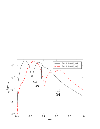
FIG. 1.: Gravitational radiation from a particle scattered by a nonrotating black hole. The particle’s energy per mass is $E=2$ and its angular momentum per mass is $L=10$, so that the orbital turning point (minimum radius) is $r_{t}=10M/3$. (a) The energy spectrum for $l=2$ and $l=3$ radiation. Arrows indicate the oscillation frequency (i.e. , real part of the QN frequency) for the least damped $l=2$ mode ($\omega M=.374$) and the least damped $l=3$ ($\omega M=.599$) modes. (b) The $l=2$ waveform in the equatorial ($\theta=\pi/2$) plane. The real part of the wavefunction $Q_{21}$ is shown; this corresponds to the waveform seen at azimuthal angle $\varphi=\pi/2$.

FIG. 2.: The full waveform as seen by observers in the plane were the particle moves ($\theta=\pi/2$). The background spacetime is a homogeneous star of radius $R=3.125M$ and the energy of the particle is $E=2$ with an angular momentum $L=10M$. The waveform as seen in the same plane in the direction $\varphi=\pi/2$ is shown below in Fig. 5(b). The middle part (spiral part) represents the ringing part of the wave. The inner (center) the tail. The outer part is the initial burst. In the figure, the $\varphi=0$ symmetry axis of the particle orbit is the line $y=r^{*}\sin\varphi=0$.

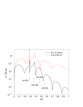
FIG. 3.: Gravitational radiation from a particle scattered by a homogeneous star of radius $R=2.33M$. (a) Absolute value of the imaginary part of $Q_{21}$ in a linear-log scale for a particle with parameters $E=2,L=10M$ and turning point $10M/3$. (b) The energy spectra for the same particle and for a particle with a lower energy ($E=1.2,L=6M$ and turning point $r_{t}=5.163M$). The four lowest damped $l=2$ QN modes, with frequencies $\omega_{I}M=0.281+i0.00014$, $\omega_{II}M=0.372+i0.0048$, $\omega_{III}M=0.458+i0.025$ and $\omega_{IV}M=0.554+i0.049$ are indicated by arrows.

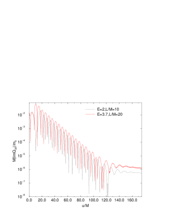
FIG. 4.: In (a) the absolute value of the $l=2$ waveform of figure 1.b is plotted in a linear-log display. The $l=3$ waveform in the plane $\theta=\pi/2$ and direction $\varphi=0$, is shown in (b) along with the $l=3$ waveform for an orbit with $E=3.7$, $L=20M$, and $r_{t}=3.768M$.

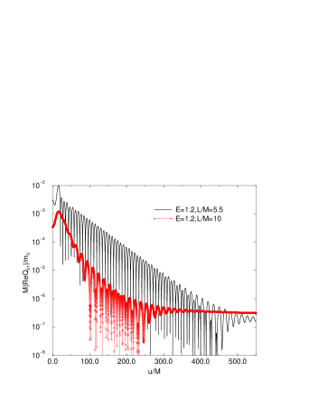
FIG. 5.: The real part of the $l=2,m=1$ odd parity waveform $Q_{21}$, for a constant density star with $R=2.5M$. The waveforms in (a) are for two orbits with $E=1.2$. The low $L$ orbit has $L=5.5M$, $r_{t}=4.047M$, and a particle frequency $d\varphi/dt=0.142M^{-1}$; the high $L$ orbit has $L=10M$, $r_{t}=11.633M$, and a particle frequency $d\varphi/dt=0.051M^{-1}$. The waveforms in (b) are for two orbits with $E=2$. The low $L$ orbit has $L=10M$, $r_{t}=10M/3$, and a particle frequency $d\varphi/dt=0.180M^{-1}$; the high $L$ orbit has $L=30M$, $r_{t}=15.862M$, and a particle frequency $d\varphi/dt=0.052M^{-1}$. The least damped ($l=2$) odd parity QN mode of this star has frequency $\omega M=0.412+i0.0219$.

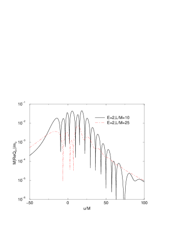
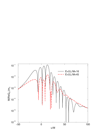
FIG. 6.: The real part of the $l=2,m=1$ odd parity waveform $Q_{21}$, for a constant density star with $R=3.125M$. The waveforms in (a) are for two orbits with $E=2$. The waveform with pronounced QN ringing has $L=10M$, $r_{t}=10M/3$ and a particle frequency $d\varphi/dt=0.180M^{-1}$; the waveform with weak QN ringing has $L=25M$, $r_{t}=12.94M$ and $d\varphi/dt=0.063M^{-1}$. The waveforms in (b) are for particle orbits with $E=3$. The waveform with strong QN ringing corresponds to a particle orbit with $L=16M$, $r_{t}=3.729M$ and $d\varphi/dt=0.178M^{-1}$; the waveform with weak ringing corresponds to a particle orbit with $L=45M$, $r_{t}=14.66M$ and $d\varphi/dt=0.0603M^{-1}$. The strong ringing part can be fitted with precision better than 1% by an oscillating damped function with the frequency of the lowest $l=2$ QN mode which is $\omega M=0.455+i0.1386$.

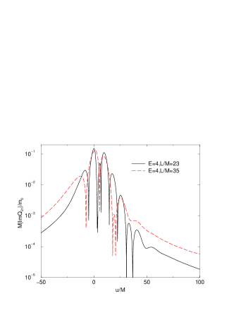
FIG. 7.: The real part of the $l=2,m=1$ odd parity waveform $Q_{21}$, for a constant density star with $R=4M$. The waveforms in (a) are for two orbits with $E=2$. The waveform with pronounced QN ringing has $L=11M$, $r_{t}=4.34M$ and a particle frequency $d\varphi/dt=0.157M^{-1}$; the waveform with no evidence of QN ringing has $L=25M$, $r_{t}=12.94M$ and $d\varphi/dt=0.0631M^{-1}$. The waveforms in (b) are for particle orbits with $E=4$. The waveform with strong QN ringing corresponds to a particle orbit with $L=23M$, $r_{t}=4.259M$ and $d\varphi/dt=0.1682M^{-1}$; the waveform with weak ringing corresponds to a particle orbit with $L=35M$, $r_{t}=7.71M$ and $d\varphi/dt=0.109M^{-1}$. For a constant density star with $R=4$ the least damped odd parity ($l=2$) QN mode has frequency $\omega M=0.401+i0.209$.

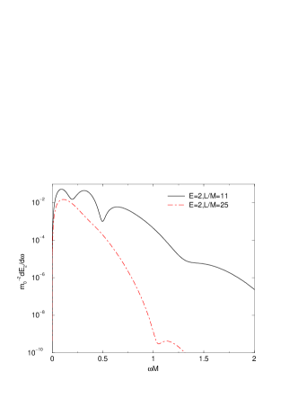
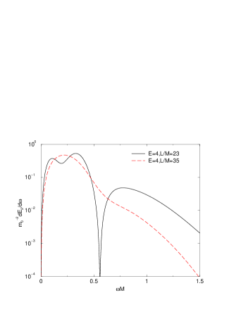
FIG. 8.: The energy spectra for the case depicted in the previous figure. The background spacetime is a homogeneous star of radius $R=4M$.

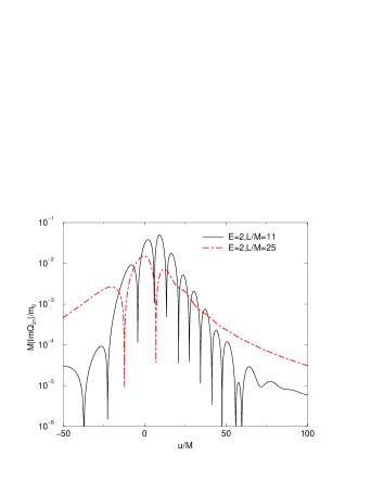
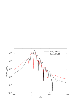
FIG. 9.: The absolute value of the imaginary part of the odd parity quadrupole waveform $Q_{21}$ is shown for a polytropic star of index $n=1$ and $K=100Km^{2}$. The central density of this star, $\rho_{0}=5\times 10^{15}g/cm^{3}$ and the radius is $R=3.91M$. In (a) the scattered particle has energy $E=2$ and two angular momenta, $L=11M$ (turning point 4.344M,$d\varphi/dt=0.157M^{-1}$) and $L=25M$ (turning point $12.943M$,$d\varphi/dt=0.063M^{-1}$) are considered. In (b), a higher energy ($E=4$) is considered and also the waveform for two angular momenta are shown: $L=23M$ (turning point 4.259M,$d\varphi/dt=0.168M^{-1}$) and $L=35M$ (turning point is 7.71M,$d\varphi/dt=0.109M^{-1}$).

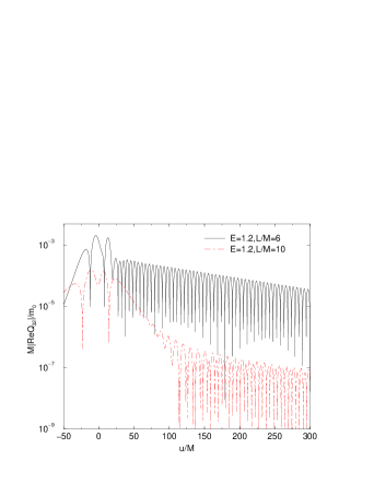
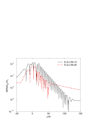
FIG. 10.: The absolute value of the real part of the odd parity octupole waveform $Q_{32}$ is shown for a homogeneous star of radius $R=2.5M$ in (a) and of radius $R=3.125M$ in (b). In (a) we consider a particle with small energy ($E=1.2$) and two angular momenta: $L=6M$ (turning point is 5.163M,$2d\varphi/dt=0.23M^{-1}$) and $L=10M$ (turning point is 11.633M, $2d\varphi/dt=0.102M^{-1}$). The amplitude of the wave for the far orbit is so small that the ringing observed (at about twice the frequency of the QN mode) is probably numerical error. In (b) we consider a particle with energy ($E=2$) and two angular momenta: $L=10M$ (turning point is 10M/3M,$2d\varphi/dt=0.36M^{-1}$) and $L=20M$ (turning point is 10M,$2d\varphi/dt=0.16M^{-1}$) moving outside a star with radius $R=3.125M$. There is, for both angular momenta, excitation of a QN mode of the star, that most likely is the lowest damped $l=3$ odd mode (from the graphic for the smaller angular momentum orbit we get $\omega M=0.691+i0.143$).

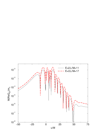
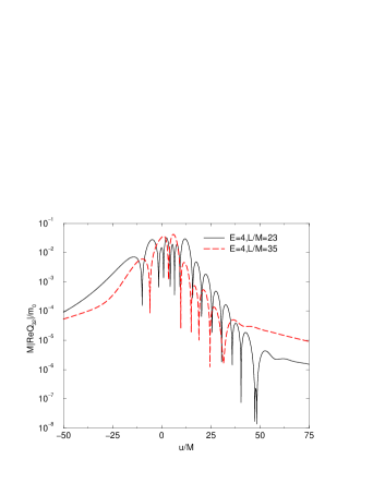
FIG. 11.: The absolute value of the real part of the odd parity octupole waveform $Q_{32}$ is shown for an homogeneous star of radius $R=4M$. In (a) we consider two sets of parameters for the particle: $E=2,L=11M$ (turning point is 4.343M, $2d\varphi/dt=0.315M^{-1}$) and $E=3,L=17M$ (turning point at 4.25M, $2d\varphi/dt=0.333M^{-1}$). In both cases ringing at the same frequency is visible (that frequency is approximately $\omega=0.64+i0.23$. In (b) the particle has energy $E=4$ and we consider two angular momenta: $L=23$ (turning point $r_{t}=4.259M$,$2d\varphi/dt=0.336M^{-1}$) and $L=35M$ (turning point 7.71M, $2d\varphi/dt=0.22M^{-1}$). In both cases there is ringing. The oscillation is clear enough for the smaller turning point to allow us to obtain its complex frequency: $\omega M=0.64+i0.23$.

REFERENCES

- [1] K. Oohara and T. Nakamura, Prog. Theor. Phys. 71, 91 (1984).
- [2] K. Oohara, Prog. Theor. Phys. 71, 738 (1984).
- [3] S. L. Detweiler and E. Szedenits, Ap. J. 231, 211 (1979).
- [4] R. F. Stark and T. Piran, Phys. Rev. Lett. 55,891(1985). Also: Errata, Phys. Rev. Lett. 56,97(1986).
- [5] The Grand Challenge Binary Black hole Alliance, see http://www.npac.syr.edu/projects/bbh, also Phys. Rev. Lett. 80, 3915, 2512 and 1812 (1998); Science, 270, 941 (1995).
- [6] Y. Kojima, Prog. Theor. Phys. 79, 665 (1988).
- [7] K. D. Kokkotas and B. Schutz, Mon. Not. R. Astron. Soc. 255, 119 (1992).
- [8] There is a single exception to this rule. The angular momentum of the fluid is an odd-parity dipole perturbation. This perturbation, however, is not radiatable, and is irrelevant to the considerations of this paper.
- [9] S. Chandrasekhar and V. Ferrari, Proc. R. Soc. Lond. A 434, 449 (1991).
- [10] N. Andersson, Y. Kojima and K. Kokkotas, Ap. J. 462, 855 (1996).
- [11] N. Andersson and K. D. Kokkotas, Mon. Not. R. Astron. Soc. 297, 493 (1998).
- [12] O. Benhar, E. Berti and V. Ferrari, gr-qc/9901037.
- [13] K. D. Kokkotas, T. A. Apostolatos and N. Andersson, gr-qc/9901072.
- [14] N. Andersson and K. D. Kokkotas, Phys. Rev. Lett. 77, 4134 (1996).
- [15] K. Tominaga, M. Saijo and K. Maeda,gr-qc/9901040.
- [16] V. Ferrari, L. Gualtieri and A. Borrelli, gr-qc/9901060.
- [17] R. F. Tooper, Ap. J. 140, 434 (1964).
- [18] F. J. Zerilli, Phys. Rev. D 2, 2141 (1970).
- [19] K. Thorne and A. Campolattaro, Ap. J. 149, 591 (1967).
- [20] T. Regge and J. A. Wheeler, Phys. Rev. 108, 1063 (1957).
- [21] V. Moncrief, Ann. Phys. (NY) 88, 323 (1974).
- [22] C. T. Cunningham, R. H. Price and V. Moncrief, Ap. J 224, 643 (1978).
- [23] C. O. Lousto and R. H. Price, Phys. Rev. D 55, 2124 (1997).
- [24] H.-P. Nollert and R. H. Price, J. Math. Phys. 40, 980 (1999).
- [25] K. Rosquist, Phys. Rev. D 59, 044022 (1999).
- [26] L. Lindblom, Phys. Rev. D 58, 024008 (1998).
- [27] C. W. Misner, K. S. Thorne, and J. A. Wheeler, Gravitation (W. H. Freeman, San Francisco, 1973).
- [28] S. Chandrasekhar,The mathematical theory of black holes , (Oxford Univ. Press, Oxford, 1983).