Lorentz Covariant Theory of Light Propagation in Gravitational Fields of Arbitrary-Moving Bodies

Abstract

The Lorentz covariant theory of propagation of light in the (weak) gravitational fields of N-body systems consisting of arbitrarily moving point-like bodies with constant masses $m_{a}$ ($a=1,2,...,N$) is constructed. The theory is based on the Liénard-Wiechert representation of the metric tensor which describes a retarded type solution of the gravitational field equations. A new approach for integrating the equations of motion of light particles (photons) depending on the retarded time argument is invented. Its application in the first post-Minkowskian approximation, which is linear with respect to the universal gravitational constant, G, makes it evident that the equations of light propagation admit to be integrated straightforwardly by quadratures. Explicit expressions for the trajectory of light ray and its tangent vector are obtained in algebraically closed form in terms of functionals of the retarded time. General expressions for the relativistic time delay, the angle of light deflection, and the gravitational shift of electromagnetic frequency are derived in the form of instantaneous functions of the retarded time. They generalize previously known results for the case of static or uniformly moving bodies. The most important applications of the theory to relativistic astrophysics and astrometry are given. They include a discussion of the velocity dependent terms in the gravitational lens equation, the Shapiro time delay in binary pulsars, gravitational Doppler shift, and a precise theoretical formulation of the general relativistic algorithms of data processing of radio and optical astrometric measurements made in the non-stationary gravitational field of the solar system. Finally, proposals for future theoretical work being important for astrophysical applications are formulated.

Contents

toc

I Introduction and Summary

The exact solution of the problem of propagation of electromagnetic waves in non-stationary gravitational fields is extremely important for modern relativistic astrophysics and fundamental astrometry. Until now it are electromagnetic signals coming from various astronomical objects which deliver the most exhaustive and accurate physical information about numerous intriguing phenomena going on in the surrounding universe. Present day technology has achieved a level at which the extremely high precision of current ground-based radio interferometric astronomical observations approaches 1 $\mu$arcsec. This requires a better theoretical treatment of secondary effects in the propagation of electromagnetic signals in variable gravitational fields of oscillating and precessing stars, stationary and coalescing binary systems, and colliding galaxies [1]. Future space astrometric missions like GAIA [2] or SIM [3] will also have precision of about 1-10 $\mu$arcsec on positions and parallaxes of stars, and about 1-10 $\mu$arcsec per year for their proper motion. At this level of accuracy we are not allowed anymore to treat the gravitational field of the solar system as static and spherically symmetric. Rotation and oblateness of the Sun and large planets as well as time variability of the gravitational field should be seriously taken into account [4].

As far as we know, all approaches developed for integrating equations of propagation of electromagnetic signals in gravitational fields were based on the usage of the post-Newtonian presentation of the metric tensor of the gravitational field. It is well-known (see, for instance, the textbooks [5], [6]) that the post-Newtonian approximation for the metric tensor is valid only within the so-called ”near zone”. Hence, the post-Newtonian metric can be used for the calculation of light propagation only from the sources lying inside the near zone of a gravitating system of bodies. The near zone is restricted by the distance comparable to the wavelength of the gravitational radiation emitted from the system. For example, Jupiter orbiting the Sun emits gravitational waves with wavelength of about 0.3 parsecs, and the binary pulsar PSR B1913+16 radiates gravitational waves with wavelength of around 4.4 astronomical units. It is obvious that the majority of stars, quasars, and other sources of electromagnetic radiation are usually far beyond the boundary of the near zone of the gravitating system of bodies and another method of solving the problem of propagation of light from these sources to the observer at the Earth should be applied. Unfortunately, such an advanced technique has not yet been developed and researches relied upon the post-Newtonian approximation of the metric tensor assuming implicitly that perturbations from the gravitational-wave part of the metric are small and may be neglected in the data processing algorithms [5], [7] - [9]. However, neither this assumption was ever scrutinized nor the magnitude of the neglected residual terms was estimated. An attempt to clarify this question has been undertaken in the paper [4] where the matching of asymptotics of the internal near zone and external Schwarzschild solutions of equations of light propagation in the gravitational field of the solar system has been employed. Nevertheless, a rigorous solution of the equations of light propagation being simultaneously valid both far outside and inside the solar system was not found.

One additional problem to be enlightened relates to how to treat the motion of gravitating bodies during the time of propagation of light from the point of emission to the point of observation. The post-Newtonian metric of a gravitating system of bodies is not static and the bodies move while light is propagating. Usually, it was presupposed that the biggest influence on the light ray the body exerts when the photon passes nearest to it. For this reason, coordinates of gravitating bodies in the post-Newtonian metric were assumed to be fixed at a specific instant of time $t_{a}$ (see, for instance, [8] - [10]) being close to that of the closest approach of the photon to the body. Nonetheless, it was never fully clear how to specify the moment $t_{a}$ precisely and what magnitude of error in the calculation of relativistic time delay and/or the light deflection angle one makes if one choses a slightly different moment of time. Previous researches gave us different conceivable prescriptions for choosing $t_{a}$ which might be used in practice. Perhaps, the most fruitful suggestion was that given by Hellings [10] and discussed later on in a paper [4] in more detail. This was just to accept $t_{a}$ as to be exactly the time of the closest approach of the photon to the gravitating body deflecting the light. Klioner & Kopeikin [4] have shown that such a choice minimizes residual terms in the solution of equation of propagation of light rays obtained by the asymptotic matching technique. We note, however, that neither Hellings [10] nor Klioner & Kopeikin [4] have justified that the choice for $t_{a}$ they made is unique.

Quite recently we have started the reconsideration of the problem of propagation of light rays in variable gravitational fields of gravitating system of bodies. First of all, a profound, systematic approach to integration of light geodesic equations in arbitrary time-dependent gravitational fields possessing a multipole decomposition [1], [11] has been worked out. A special technique of integration of the equation of light propagation with retarded time argument has been developed which allowed to discover a rigorous solution of the equations everywhere outside a localized source emitting gravitational waves. The present paper continues the elaboration of the technique and makes it clear how to construct a Lorentz covariant solution of equations of propagation of light rays both outside and inside of a gravitating system of massive point-like particles moving along arbitrary world lines. In finding the solution we used the Liénard-Wiechert presentation for the metric tensor which accounts for all possible effects in the description of the gravitational field and is valid everywhere outside the world lines of the bodies. The solution, we have found, allows to give an unambiguous theoretical prescription for chosing the time $t_{a}$. In addition, by a straightforward calculation we obtain the complete expressions for the angle of light deflection, relativistic time delay (Shapiro effect), and gravitational shift of observed electromagnetic frequency of the emitted photons. These expressions are exact at the linear approximation with respect to the universal gravitational constant, $G$, and at arbitrary order of magnitude with respect to the parameter $v_{a}/c$ where $v_{a}$ is a characteristic velocity of the $a$-th light-deflecting body, and $c$ is the speed of light [12]. We devote a large part of the paper to the discussion of practical applications of the new solution of the equations of light propagation including moving gravitational lenses, timing of binary pulsars, the consensus model of very long baseline interferometry, and the relativistic reduction of astrometric observations in the solar system.

The formalism of the present paper can be also used in astrometric experiments for testing alternative scalar-tensor theories of gravity after formal replacing in all subsequent formulas the universal gravitational constant $G$ by the product $G(\gamma^{\ast}+1)/2$, where $\gamma^{\ast}$ is the effective light-deflection parameter which is slightly different from its weak-field limiting value $\gamma$ of the standard parameterized post-Newtonian (PPN) formalism [13]. This statement is a direct consequence of a conformal invariance of equations of light rays [16] and can be immediately proved by straightforward calculations. Solar system experiments have not been sensitive enough to detect the difference between the two parameters. However, it may play a role in the binary pulsars analysis [14].

The paper is organized as follows. Section 2 presents a short description of the energy-momentum tensor of the light-deflecting bodies and the metric tensor given in the form of the Liénard-Wiechert potential. Section 3 is devoted to the development of a mathematical technique for integrating equations of propagation of electromagnetic waves in the geometric optics approximation. Solution of these equations and relativistic perturbations of a photon trajectory are given in Section 4. We briefly outline equations of motion for slowly moving observers and sources of light in Section 5. Section 6 deals with a general treatment of observable relativistic effects - the integrated time delay, the deflection angle, and gravitational shift of frequency. Particular cases are presented in Section 7. They include the Shapiro time delay in binary pulsars, moving gravitational lenses, and general relativistic astrometry in the solar system.

II Energy-Momentum and Metric Tensors

The tensor of energy-momentum of a system of massive particles is given in covariant form, for example, by Landau & Lifshitz [17]

$$T^{\alpha\beta}(t,{\bf x}) = \sum_{a=1}^{N}\hat{T}_{a}^{\alpha\beta}(t)\delta\left({\bf x}-{\bf x}_{a}(t)\right)\;,$$ (1)

$$\hat{T}_{a}^{\alpha\beta}(t) = m_{a}\gamma_{a}^{-1}(t)u_{a}^{\alpha}(t)u_{a}^{\beta}(t)\;,$$ (3)

where $t$ is coordinate time, ${\bf x}=x^{i}=(x^{1},x^{2},x^{3})$ denotes spatial coordinates of a current point in space, $m_{a}$ is the constant (relativistic) rest mass of the $a$-th particle, ${\bf x}_{a}(t)$ are spatial coordinates of the $a$-th massive particle which depend on time $t$, ${\bf v}_{a}(t)=d{\bf x}_{a}(t)/dt$ is velocity of the $a$-th particle, $\gamma_{a}(t)=[1-v_{a}^{2}(t)]^{-1/2}$ is the (time-dependent) Lorentz factor, $u_{a}^{\alpha}(t)=\{\gamma_{a}(t),\;\gamma_{a}(t){\bf v}_{a}(t)\}$ is the four-velocity of the $a$-th particle, $\delta({\bf x})$ is the usual 3-dimensional Dirac delta-function. In particular, we have

$$\hat{T}_{a}^{00}(t)=\frac{m_{a}}{\sqrt{1-v_{a}^{2}(t)}}\;,\hskip 42.67912pt\hat{T}_{a}^{0i}(t)=\frac{m_{a}v_{a}^{i}(t)}{\sqrt{1-v_{a}^{2}(t)}}\;,\hskip 42.67912pt\hat{T}_{a}^{ij}(t)=\frac{m_{a}v_{a}^{i}(t)v_{a}^{j}(t)}{\sqrt{1-v_{a}^{2}(t)}}\;.\hskip 42.67912pt$$ (5)

The metric tensor in the linear approximation reads

$$g_{\alpha\beta}(t,{\bf x}) = \eta_{\alpha\beta}+h_{\alpha\beta}(t,{\bf x})\;,$$ (6)

where $\eta_{\alpha\beta}={\rm diag}(-1,+1,+1,+1)$ is the Minkowski metric of flat space-time and the metric perturbation $h_{\alpha\beta}(t,{\bf x})$ is a function of time and spatial coordinates [18]. It can be found by solving the Einstein field equations which read in the first post-Minkowskian approximation and in the harmonic gauge [19] as follows ([20], chapter 10)

$$\mathop{\kern 1.0pt\hbox{${\vbox{\hrule height=0.4pt\hbox{\vrule width=0.4pt,height=8.0pt\kern 8.0pt\vrule width=0.4pt} \hrule height=0.4pt}}$}\kern 1.0pt}h_{\alpha\beta}(t,{\bf x}) = -16\pi S_{\alpha\beta}(t,{\bf x})\;,$$ (8)

where

$$S_{\alpha\beta}(t,{\bf x}) = T_{\alpha\beta}(t,{\bf x})-\frac{1}{2}\eta_{\alpha\beta}\;T_{\;\;\lambda}^{\lambda}(t,{\bf x})\;.$$ (9)

The solution of this equations has the form of the Liénard-Wiechert potential [21]. In order to see how it looks like we represent the tensor of energy-momentum in a form where all time dependence is included in a one-dimensional delta-function

$$T^{\alpha\beta}(t,{\bf x}) = \int_{-\infty}^{+\infty}dt^{\prime}\delta(t^{\prime}-t)\ T^{\alpha\beta}(t^{\prime},{\bf x})\;.$$ (11)

Here $t^{\prime}$ is an independent parameter along the world lines of the particles which does not depend on time $t$. The solution of equation (8) can be found using the retarded Green function [22], and after integration with respect to spatial coordinates, using the 3-dimensional delta-function, it is given in the form of an one-dimensional retarded-time integral

$$h^{\alpha\beta}(t,{\bf x}) = \sum_{a=1}^{N}\int_{-\infty}^{+\infty}\hat{h}^{\alpha\beta}_{a}(t^{\prime},t,{\bf x})dt^{\prime}\;,$$ (12)

$$\hat{h}^{\alpha\beta}_{a}(t^{\prime},t,{\bf x}) = 4\left[\hat{T}_{a}^{\alpha\beta}(t^{\prime})-\frac{1}{2}\eta^{\alpha\beta}\hat{T}_{a\lambda}^{\lambda}(t^{\prime})\right]\frac{\delta\left[t^{\prime}-t+r_{a}(t^{\prime})\right]}{r_{a}(t^{\prime})}\;,$$ (14)

where ${\bf r}_{a}(t^{\prime})={\bf x}-{\bf x}_{a}(t^{\prime})$, and $r_{a}(t^{\prime})=|{\bf r}_{a}(t^{\prime})|$ is the usual Euclidean length of the vector.

The integral (12) can be performed explicitly as described in, e.g., ([21], section 14). The result is the retarded Liénard-Wiechert tensor potential

$$h^{\alpha\beta}(t,{\bf x}) = 4\sum_{a=1}^{N}\;\frac{\hat{T}_{a}^{\alpha\beta}(s)-\frac{1}{2}\eta^{\alpha\beta}\hat{T}_{a\lambda}^{\lambda}(s)}{r_{a}(s)-{\bf v}_{a}(s)\cdot{\bf r}_{a}(s)}\;,$$ (16)

where the retarded time $s=s(t,{\bf x})$ for the $a$-th body is a solution of the light-cone equation [26]

$$s+|{\bf x}-{\bf x}_{a}(s)| = t\;.$$ (17)

Here it is assumed that the field is measured at time $t$ and at the point ${\bf x}$. We shall use this form of the metric perturbation $h_{\alpha\beta}(t,{\bf x})$ for the integration of the equations of light geodesics in the next section. It is worth emphasizing that the expression for the metric tensor (16) is Lorentz-covariant and is valid in any harmonic coordinate system admitting a smooth transition to the asymptotically flat space-time at infinity and relating to each other by the Lorentz transformations of theory of special relativity [6], [27]. A treatment of post-linear corrections to the Liénard-Wiechert potentials (16) is given, for example, in a series of papers by Kip Thorne and collaborators [28], [31] - [33].

III Mathematical Technique for Integrating Equations of Propagation of Photons

We consider the motion of a light particle (photon) in the background gravitational field described by the metric (12). No back action of the photon on the gravitational field is assumed. Hence, we are allowed to use equations of light geodesics directly applying the metric tensor in question. Let the motion of the photon be defined by fixing the mixed initial-boundary conditions (see Fig 1)

$${\bf x}(t_{0})={\bf x}_{0}\;,\hskip 56.9055pt{\displaystyle{d{\bf x}(-\infty)\over dt}}={\bf k}\;,$$ (18)

where ${\bf k}^{2}=1$ and, henceforth, the spatial components of vectors are denoted by bold letters. These conditions define the coordinates ${\bf x}_{0}$ of the photon at the moment of emission of light, $t_{0}$, and its velocity at the infinite past and infinite distance from the origin of the spatial coordinates (that is, at the, so-called, past null infinity).

The original equations of propagation of light rays are rather complicated [1]. They can be simplified and reduced to the form which will be shown later in this section. In order to integrate them we shall have to resort to a special approximation method. In the Minkowskian approximation of the flat space-time the unperturbed trajectory of the light ray is a straight line

$$x^{i}(t) = x^{i}_{N}(t)=x^{i}_{0}+k^{i}\;\left(t-t_{0}\right)\;,$$ (19)

where $t_{0}$, $x^{i}_{0}$, and $k^{i}={\bf k}$ have been defined in equation (18). In this approximation, the coordinate speed of the photon is $\dot{x}^{i}=k^{i}$ and is considered as a constant in the expression for the light-ray-perturbing force.

It is convenient to introduce a new independent parameter $\tau$ along the photon’s trajectory according to the rule [1], [11]

$$\tau = {\bf k}\cdot{\bf x}_{N}(t)=t-t_{0}+{\bf k}\cdot{\bf x}_{0},$$ (21)

where here and in the following the dot symbol $"\cdot"$ between two spatial vectors denotes the Euclidean dot product. The time $t_{0}$ of the light signal’s emission corresponds to the numerical value of the parameter $\tau_{0}={\bf k}\cdot{\bf x}_{0}$, and the numerical value of the parameter $\tau=0$ corresponds to the time

$$t^{\ast} = t_{0}-{\bf k}\cdot{\bf x}_{0}\;,$$ (22)

which is the time of the closest approach of the unperturbed trajectory of the photon to the origin of an asymptotically flat harmonic coordinate system. We emphasize that the numerical value of the moment $t^{\ast}$ is constant for a chosen trajectory of light ray and depends only on the space-time coordinates of the point of emission of the photon and the point of its observation. Thus, we find the relationships

$$\tau \equiv t-t^{\ast},\hskip 56.9055pt\tau_{0}=t_{0}-t^{\ast}\;,$$ (23)

which reveals that the variable $\tau$ is negative from the point of emission up to the point of the closest approach $x^{i}(t^{\ast})=\hat{\xi}^{i}$, and is positive otherwise [34]. The differential identity $dt=d\tau$ is valid and, for this reason, the integration along the light ray’s path with respect to time $t$ can be always replaced by the integration with respect to variable $\tau$.

Making use of the parameter $\tau$, the equation of the unperturbed trajectory of the light ray can be represented as

$$x^{i}(\tau) = x^{i}_{N}(\tau)=k^{i}\tau+\hat{\xi}^{i}\;,$$ (24)

and the distance, $r(\tau)=|{\bf x}_{N}(t)|$, of the photon from the origin of the coordinate system reads

$$r(\tau) = \sqrt{\tau^{2}+d^{2}}\;.$$ (25)

The constant vector $\hat{\xi}^{i}={\hat{\mbox{\boldmath$\xi$}}}={\bf k}\times({\bf x}_{0}\times{\bf k})={\bf k}\times\left({\bf x}_{N}(t)\times{\bf k}\right)$ is called the impact parameter of the unperturbed trajectrory of the light ray, $d=|{\hat{\mbox{\boldmath$\xi$}}}|$ is the length of the impact parameter, and the symbol $"\times"$ between two vectors denotes the usual Euclidean cross product of two vectors. We note that the vector ${\hat{\mbox{\boldmath$\xi$}}}$ is transverse to the vector ${\bf k}$. It is worth emphasizing once again that the vector $\hat{\xi}^{i}$ is directed from the origin of the coordinate system towards the point of the closest approach of the unperturbed path of the light ray to the origin. This vector plays an auxiliary role in our discussion and, in general, has no essential physical meaning as it can be easily changed by the shift of the origin of the coordinates [35].

Implementing the two new parameters $\tau$, ${\hat{\mbox{\boldmath$\xi$}}}$ and introducing the four-dimensional isotropic vector $k^{\alpha}=(1,k^{i})$ one can write the equations of light geodesics as follows (for more details see the paper [1] and reference [36])

$$\ddot{x}^{i}(\tau) = \frac{1}{2}k_{\alpha}k_{\beta}{\hat{\partial}}_{i}h^{\alpha\beta}(\tau,{\hat{\mbox{\boldmath$\xi$}}})-{\hat{\partial}}_{\tau}\left[k_{\alpha}h^{\alpha i}(\tau,{\hat{\mbox{\boldmath$\xi$}}})+\frac{1}{2}k^{i}h^{00}(\tau,{\hat{\mbox{\boldmath$\xi$}}})-\frac{1}{2}k^{i}k_{p}k_{q}h^{pq}(\tau,{\hat{\mbox{\boldmath$\xi$}}})\right]\;,$$ (26)

where dots over the coordinates denote differentiation with respect to time, ${\hat{\partial}}_{\tau}\equiv\partial/\partial\tau$, ${\hat{\partial}}_{i}\equiv P_{ij}\partial/\partial\hat{\xi}^{j}$, and $P_{ij}=\delta_{ij}-k_{i}k_{j}$ is the operator of projection onto the plane being orthogonal to the vector $k^{i}$, and all quantities on the right hand side of equation (26) are taken along the light trajectory at the point corresponding to a numerical value of the running parameter $\tau$ while the parameter $\hat{\mbox{\boldmath$\xi$}}$ is assumed as constant. Hence, the equation (26) should be considered as an ordinary, second order differential equation in variable $\tau$ [37]. The given form of equation (26) already shows that only the first term on the right hand side of it can contribute to the deflection of light if the observer and the source of light are at spatial infinity. Indeed, a first integration of the right hand side of the equation (26) with respect to time from $-\infty$ to $+\infty$ brings all terms showing time derivatives to zero due to the asymptotic flatness of the metric tensor which proves our statement (for more details see the next section).

However, if the observer and the source of light are located at finite distances from the origin of coordinate system, we need to know how to perform the integrals from the metric perturbations (12) with respect to the parameter $\tau$ along the unperturbed trajectory of light ray. Let us denote those integrals as

$$B^{\alpha\beta}(\tau,{\hat{\mbox{\boldmath$\xi$}}}) = \int_{-\infty}^{\tau}h^{\alpha\beta}[\sigma,{\bf x}(\sigma)]d\sigma\;,$$ (28)

$$D^{\alpha\beta}(\tau,{\hat{\mbox{\boldmath$\xi$}}}) = \int_{-\infty}^{\tau}B^{\alpha\beta}(\sigma,{\hat{\mbox{\boldmath$\xi$}}})d\sigma\;,$$ (30)

where the metric perturbation $h^{\alpha\beta}[\sigma,{\bf x}(\sigma)]$ is defined by the Liénard-Wiechert potential (12) and $\sigma$ is a parameter along the light ray having the same meaning as the parameter $\tau$ in equation (21). In order to calculate the integrals (28), (30) it is useful to change in the integrands the time argument, $\sigma$, to the new one, $\zeta$, defined by the light-cone equation (17) which after substitution for ${\bf x}$ the unperturbed light trajectory (24) reads as follows [45]

$$\sigma+t^{\ast}=\zeta+|{\hat{\mbox{\boldmath$\xi$}}}+{\bf k}\sigma-{\bf x}_{a}(\zeta)|\;.\\$$ (32)

The differentiation of this equation yields a relationship between differentials of the time variables $\sigma$ and $\zeta$, and parameters $t^{\ast}$, $\xi^{i}$, $k^{i}$

$$d\zeta\left(r_{a}-{\bf v}_{a}\cdot{\bf r}_{a}\right)=d\sigma\left(r_{a}-{\bf k}\cdot{\bf r}_{a}\right)+r_{a}dt^{\ast}-{\bf r}_{a}\cdot d{\hat{\mbox{\boldmath$\xi$}}}-\sigma{\bf r}_{a}\cdot d{\bf k}\;,\\$$ (33)

where the coordinates, ${\bf x}_{a}$, and the velocity, ${\bf v}_{a}$, of the $a$-th body are taken at the retarded time $\zeta$, and coordinates of the photon, ${\bf x}$, are taken at the time $\sigma(\zeta)$. From equation (33) we immediately obtain the partial derivatives with respect to the parameters

$$\frac{\partial\zeta}{\partial t^{\ast}}=\frac{r_{a}}{r_{a}-{\bf v}_{a}\cdot{\bf r}_{a}}\;,\quad\quad\quad\frac{\partial\zeta}{\partial\hat{\xi}^{i}}=-\frac{P_{ij}r_{a}^{j}}{r_{a}-{\bf v}_{a}\cdot{\bf r}_{a}}\;,\quad\quad\quad\frac{\partial\zeta}{\partial k^{i}}=-\frac{\sigma r_{a}^{i}}{r_{a}-{\bf v}_{a}\cdot{\bf r}_{a}}\;,\\$$ (34)

and have the relationship between the time differentials along the world line of the photon which reads as follows

$$d\sigma=d\zeta\;\frac{r_{a}-{\bf v}_{a}\cdot{\bf r}_{a}}{r_{a}-{\bf k}\cdot{\bf r}_{a}}\;.\\$$ (35)

If the parameter $\sigma$ runs from $-\infty$ to $+\infty$, the new parameter $\zeta$ runs from $\zeta_{-\infty}=-\infty$ to $\zeta_{+\infty}=t^{\ast}+{\bf k}\cdot{\bf x}_{a}(\zeta_{+\infty})$ provided the motion of each body is restricted inside a bounded domain of space, like in the case of a binary system. In case the bodies move along straight lines with constant velocities, the parameter $\sigma$ runs from $-\infty$ to $+\infty$, and the parameter $\zeta$ runs from $-\infty$ to $+\infty$ as well. In addition, we note that when the numerical value of the parameter $\sigma$ is equal to the time of observation $\tau$, the numerical value of the parameter $\zeta$ equals to $s(\tau)$, which is found from the equation of the light cone (17) in which the point ${\bf x}$ denotes spatial coordinates of observer.

After transforming time arguments the integrals (28), (30) take the form

$$B^{\alpha\beta}(s)=\sum_{a=1}^{N}B^{\alpha\beta}_{a}(s)\;,\quad\quad\quad B^{\alpha\beta}_{a}(s)=4\int_{-\infty}^{s}\frac{\hat{T}_{a}^{\alpha\beta}(\zeta)-\frac{1}{2}\eta^{\alpha\beta}\hat{T}_{a\lambda}^{\lambda}(\zeta)}{r_{a}(\sigma,\zeta)-{\bf k}\cdot{\bf r}_{a}(\sigma,\zeta)}d\zeta\;,$$ (36)

$$D^{\alpha\beta}(s) = \sum_{a=1}^{N}\int_{-\infty}^{\tau}B^{\alpha\beta}_{a}[\zeta(\sigma)]d\sigma\;,$$ (37)

where retarded times in the upper limits of integration depend on the index of each body as it has already been mentioned in the previous text. Now we give a remarkable, exact relationship

$$r_{a}(\sigma,\zeta)-{\bf k}\cdot{\bf r}_{a}(\sigma,\zeta)=t^{\ast}+{\bf k}\cdot{\bf x}_{a}(\zeta)-\zeta\;,\\$$ (39)

which can be proved by direct use of the light-cone equation (17) and the expression (24) for the unperturbed trajectory of light ray. It is important to note that in the given relationship $t^{\ast}$ is a constant time corresponding to the moment of the closest approach of the photon to the origin of coordinate system. The equation (39) shows that the integrand on the left hand side of the second of equations (36) does not depend on the parameter $\sigma$ at all, and the integration is performed only with respect to the retarded time variable $\zeta$. Thus, just as the law of motion of the bodies ${\bf x}_{a}(t)$ is known, the integral (36) can be calculated either analytically or numerically without solving the complicated light-cone equation (17) to establish the relationship between the ordinary and retarded time arguments. This statement is not applicable to the integral (37) because transformation to the new variable (35) does not eliminate from the integrand of this integral the explicit dependence on the argument of time $\tau$. Fortunately, as it is evident from the structure of equation (26), we do not need to calculate this integral.

Instead of that, we need to know the first spatial derivative of $D^{\alpha\beta}(s)$ with respect to $\hat{\xi}^{i}$. In order to find it we note that the integrand of $B^{\alpha\beta}(s)$ does not depend on the variable $\hat{\xi}^{i}$. This dependence manifests itself only indirectly through the upper limit $s(\tau,\xi)$ of the integral because of the structure of the light-cone equation which assumes at the point of observation the following form

$$\tau+t^{\ast} = s+|\hat{{\mbox{\boldmath$\xi$}}}+{\bf k}\tau-{\bf x}_{a}(s)|\;.$$ (40)

For this reason, a straightforward differentiation of $B^{\alpha\beta}(s)$ with respect to the retarded time $s$ and the implementation of formula (34) for the calculation of the derivative $\partial s/\partial\hat{\xi}^{i}$ at the point of observation yields [46]

$${\hat{\partial}}_{i}B^{\alpha\beta}(s) = -4\sum_{a=1}^{N}\frac{\hat{T}_{a}^{\alpha\beta}(s)-\frac{1}{2}\eta^{\alpha\beta}\hat{T}_{a\lambda}^{\lambda}(s)}{r_{a}(s)-{\bf k}\cdot{\bf r}_{a}(s)}\;\frac{P^{i}_{\;j}\;r_{a}^{j}(s)}{r_{a}(s)-{\bf v}_{a}(s)\cdot{\bf r}_{a}(s)}\;.$$ (41)

This result elucidates that ${\hat{\partial}}_{i}B^{\alpha\beta}(s)$ is not an integral but instanteneous function of time and, that it can be calculated directly if the motion of the gravitating bodies is given. While calculating ${\hat{\partial}}_{i}D^{\alpha\beta}(s)$ we use, first, the formula (41) and, then, replacement of variables (35). Proceeding in this way we arrive at the result

$${\hat{\partial}}_{i}D^{\alpha\beta}(s) = \sum_{a=1}^{N}\int_{-\infty}^{\tau}{\hat{\partial}}_{i}B^{\alpha\beta}_{a}[\zeta(\sigma)]d\sigma=-4\sum_{a=1}^{N}\int_{-\infty}^{s}\frac{\hat{T}_{a}^{\alpha\beta}(\zeta)-\frac{1}{2}\eta^{\alpha\beta}\hat{T}_{a\lambda}^{\lambda}(\zeta)}{\left[r_{a}(\sigma,\zeta)-{\bf k}\cdot{\bf r}_{a}(\sigma,\zeta)\right]^{2}}P^{i}_{\;j}\;r_{a}^{j}(\sigma,\zeta)d\zeta$$ (42)

$$= -4\sum_{a=1}^{N}\biggl{\{}\hat{\xi}^{i}\int_{-\infty}^{s}\frac{\hat{T}_{a}^{\alpha\beta}(\zeta)-\frac{1}{2}\eta^{\alpha\beta}\hat{T}_{a\lambda}^{\lambda}(\zeta)}{\left[t^{\ast}+{\bf k}\cdot{\bf x}_{a}(\zeta)-\zeta\right]^{2}}d\zeta-P^{i}_{\;j}\int_{-\infty}^{s}\frac{\hat{T}_{a}^{\alpha\beta}(\zeta)-\frac{1}{2}\eta^{\alpha\beta}\hat{T}_{a\lambda}^{\lambda}(\zeta)}{\left[t^{\ast}+{\bf k}\cdot{\bf x}_{a}(\zeta)-\zeta\right]^{2}}\;\;x^{j}_{a}(\zeta)\;d\zeta\biggr{\}}\;,$$ (44)

where the numerical value of the parameter $s$ in the upper limit of the integral is calculated by solving the light-cone equation (17). Going back to the equation (39) we find that the integrand of the integral (42) depends only on the retarded time argument $\zeta$. Hence, again, as it has been proven for $B^{\alpha\beta}(s)$, the integral (42) admits a direct calculation as soon as the motion of the gravitating bodies is prescribed [47].

IV Relativistic Perturbations of a Photon Trajectory

Perturbations of the trajectory of the photon are found by straightforward integration of the equations of light geodesics (26) using the expressions (28), (30). Performing the calculations we find

$$\dot{x}^{i}(\tau) = k^{i}+\dot{\Xi}^{i}(\tau)\;,$$ (45)

$$x^{i}(\tau) = x^{i}_{N}(\tau)+\Xi^{i}(\tau)-\Xi^{i}(\tau_{0})\;,$$ (46)

where $\tau$ and $\tau_{0}$ correspond, respectively, to the moment of observation and emission of the photon. The functions $\dot{\Xi}^{i}(\tau)$ and $\Xi^{i}(\tau)$ are given as follows

$$\dot{\Xi}^{i}(\tau) = \frac{1}{2}k_{\alpha}k_{\beta}{\hat{\partial}}_{i}B^{\alpha\beta}(\tau)-k_{\alpha}h^{\alpha i}(\tau)-\frac{1}{2}k^{i}h^{00}(\tau)+\frac{1}{2}k^{i}k_{p}k_{q}h^{pq}(\tau)\;,$$ (47)

$$\Xi^{i}(\tau) = \frac{1}{2}k_{\alpha}k_{\beta}{\hat{\partial}}_{i}D^{\alpha\beta}(\tau)-k_{\alpha}B^{\alpha i}(\tau)-\frac{1}{2}k^{i}B^{00}(\tau)+\frac{1}{2}k^{i}k_{p}k_{q}B^{pq}(\tau)\;,$$ (49)

where the functions $h^{\alpha\beta}(\tau)$, $B^{\alpha\beta}(\tau)$, ${\hat{\partial}}_{i}B^{\alpha\beta}(\tau)$, and ${\hat{\partial}}_{i}D^{\alpha\beta}(\tau)$ are defined by the relationships (16), (36), (41), and (42) respectively.

The latter equation can be used for the formulation of the boundary value problem for the equation of light geodesics. In this case the initial position, ${\bf x}_{0}={\bf x}(t_{0})$, and final position, ${\bf x}={\bf x}(t)$, of the photon are given instead of the initial position ${\bf x}_{0}$ of the photon and the direction of light propagation ${\bf k}$ given at past null infinity. All what we need for the formulation of the boundary value problem is the relationship between the unit vector ${\bf k}$ and the unit vector

$${\bf K}=-\;\frac{{\bf x}-{\bf x}_{0}}{|{\bf x}-{\bf x}_{0}|}\;,$$ (51)

which defines a geometric direction of the light propagation from observer to the source of light in flat space-time (see Fig 1). The formulas (46) and (49) yield

$$k^{i} = -K^{i}-\beta^{i}(\tau,{\hat{\mbox{\boldmath$\xi$}}})+\beta^{i}(\tau_{0},{\hat{\mbox{\boldmath$\xi$}}})\;,$$ (52)

where relativistic corrections to the vector $K^{i}$ are defined as follows

$$\beta^{i}(\tau,{\hat{\mbox{\boldmath$\xi$}}}) = \frac{\frac{1}{2}k_{\alpha}k_{\beta}{\hat{\partial}}_{i}D^{\alpha\beta}(\tau)-k_{\alpha}P^{i}_{\;j}B^{\alpha j}(\tau)}{|{\bf x}-{\bf x}_{0}|}\;,$$ (53)

$$\beta^{i}(\tau_{0},{\hat{\mbox{\boldmath$\xi$}}}) = \frac{\frac{1}{2}k_{\alpha}k_{\beta}{\hat{\partial}}_{i}D^{\alpha\beta}(\tau_{0})-k_{\alpha}P^{i}_{\;j}B^{\alpha j}(\tau_{0})}{|{\bf x}-{\bf x}_{0}|}\;.$$ (55)

We emphasize that the vectors $\beta^{i}(\tau,{\hat{\mbox{\boldmath$\xi$}}})\equiv{{\mbox{\boldmath$\beta$}}}$ and $\beta^{i}(\tau_{0},{\hat{\mbox{\boldmath$\xi$}}})\equiv{{\mbox{\boldmath$\beta$}}}_{0}$ are orthogonal to the vector ${\bf k}$ and are taken at the points of observation and emission of the photon respectively. The relationships obtained in this section are used for the discussion of observable relativistic effects in the following section.

V Equations of Motion for Moving Observers and Sources of Light

The knowledge of trajectory of motion of photons in the gravitational field formed by a N-body system of arbitrary-moving point masses is necessary but not enough for the unambiguous physical interpretation of observational effects. It also requires to know how observers and sources of light move in the gravitational field of this system. Let us assume that observer and the source of light are point-like massless particles which move along time-like geodesic world lines. Then, in the post-Minkowskian approximation equations of motion of the particles, assuming no restriction on their velocities except for that $v<c$ (see, however, discussion in [30]), read

$$\ddot{x}^{i}(t) = \frac{1}{2}h_{00,i}-h_{0i,t}-\frac{1}{2}h_{00,t}\dot{x}^{i}-h_{ik,t}\dot{x}^{k}-\left(h_{0i,k}-h_{0k,i}\right)\dot{x}^{k}$$ (57)

$$\mbox{}-h_{00,k}\dot{x}^{k}\dot{x}^{i}-\left(h_{ik,j}-\frac{1}{2}h_{kj,i}\right)\dot{x}^{k}\dot{x}^{j}+\left(\frac{1}{2}h_{kj,t}-h_{0k,j}\right)\dot{x}^{k}\dot{x}^{j}\dot{x}^{i}+O(\frac{G^{2}}{c^{4}})\;.$$

In the given coordinate system for velocities much smaller than the speed of light, the equation (57) reduces to

$$\ddot{x}^{i}(t) = \frac{1}{2}h_{00,i}+O(\frac{G}{c^{2}})+O(\frac{G^{2}}{c^{4}})\;.$$ (58)

Regarding specific physical conditions either the post-Minkowskian equation (57) or the post-Newtonian equation (58) should be integrated with respect to time to give the coordinates of an observer, ${\bf x}(t)$, and a source of light, ${\bf x}_{0}(t_{0})$, as a function of time of observation, $t$, and of time of emission of light, $t_{0}$, respectively. We do not treat this problem in the present paper as its solution has been developed with necessary accuracy by a number of previous authors. In particular, the post-Minkowskian approach for solving equations of motion of massive particles is thoroughly treated in [43], [44], [48], and references therein. The post-Newtonian approach is outlined in details, for instance, in [6], [8], [49] - [51], and references therein. In what follows, we assume the motions of observer, ${\bf x}(t)$, and source of light, ${\bf x}_{0}(t_{0})$, to be known with the required precision.

VI Observable Relativistic Effects

A Shapiro Time Delay

The relativistic time delay in propagation of electromagnetic signals passing through the static, spherically-symmetric gravitational field of the Sun was discovered by Irwin Shapiro [52]. We shall give in this paragraph the generalization of his idea for the case of the propagation of light through the non-stationary gravitational field formed by an ensemble of $N$ arbitrary-moving bodies. The result, which we shall obtain, is valid not only when the light ray propagates outside the system of the bodies but also when light goes through the system. In this sense we extend our calculations made in a previous paper [1] which treated relativistic effects in propagation of light rays only outside the gravitating system having a time-dependent quadrupole moment.

The total time of propagation of an electromagnetic signal from the point ${\bf x}_{0}$ to the point ${\bf x}$ is derived from equations (46), (49). First, we use the equation (46) to express the difference ${\bf x}-{\bf x}_{0}$ through the other terms of the equation. Then, we multiply this difference by itself using the properties of the Euclidean dot product. Finally, we find the total time of propagation of light, $t-t_{0}$, extracting the square root from the product, and using the expansion with respect to the relativistic parameter $(Gm_{a})/(c^{2}r_{a})$ which is assumed to be small. It results in

$$t-t_{0} = |{\bf x}-{\bf x}_{0}|-{\bf{k}}\cdot{{\mbox{\boldmath$\Xi$}}}(\tau)+{\bf{k}}\cdot{{\mbox{\boldmath$\Xi$}}}(\tau_{0})\;,$$ (59)

or

$$t-t_{0} = |{\bf x}-{\bf x}_{0}|+\Delta(t,t_{0})\;,$$ (60)

where $|{\bf x}-{\bf x}_{0}|$ is the usual Euclidean distance between the points of emission, ${\bf x}_{0}$, and observation, ${\bf x}$, of the photon, and $\Delta(t,t_{0})$ is the generalized Shapiro time delay produced by the gravitational field of moving bodies

$$\Delta(t,t_{0}) = \frac{1}{2}k_{\alpha}k_{\beta}B^{\alpha\beta}(\tau)-\frac{1}{2}k_{\alpha}k_{\beta}B^{\alpha\beta}(\tau_{0})\;=\;2\sum_{a=1}^{N}m_{a}\;B_{a}(s,s_{0})\;.$$ (61)

In the integral

$$B_{a}(s,s_{0}) = \displaystyle{\int^{s}_{s_{0}}}\frac{[1-{\bf k}\cdot{\bf v}_{a}(\zeta)]^{2}}{\sqrt{1-v^{2}_{a}(\zeta)}}\frac{d\zeta}{t^{\ast}+{\bf k}\cdot{\bf x}_{a}(\zeta)-\zeta}\;,$$ (62)

the retarded time $s$ is obtained by solving the equation (17) for the time of observation of the photon, and $s_{0}$ is found by solving the same equation written down for the time of emission of the photon [53]

$$s_{0}+|{\bf x}_{0}-{\bf x}_{a}(s_{0})| = t_{0}\;.$$ (63)

The relationships (60), (61) for the time delay have been derived with respect to the coordinate time $t$. The transformation from the coordinate time to the proper time ${\cal T}$ of the observer is made by integrating the infinitesimal increment of the proper time along the world line ${\bf x}(t)$ of the observer [17]

$${\cal T} = \int^{t}_{t_{\rm i}}\biggl{\{}1-{\bf v}^{2}(t)-h_{00}[t,{\bf x}(t)]-2h_{0i}[t,{\bf x}(t)]v^{i}(t)-h_{ij}[t,{\bf x}(t)]v^{i}(t)v^{j}(t)\biggr{\}}^{1/2}\;dt\;,$$ (64)

where $t_{\rm i}$ is the initial epoch of observation, and $t$ is a time of observation.

The calculation of the integral (62) is performed by means of using a new variable

$$y=t^{\ast}+{\bf k}\cdot{\bf x}_{a}(\zeta)-\zeta\;,\quad\quad\quad\quad dy=-[1-{\bf k}\cdot{\bf v}_{a}(\zeta)]d\zeta\;,$$ (65)

so that the above integral (62) reads

$$B_{a}(s,s_{0}) = -\int^{s}_{s_{0}}\frac{1-{\bf k}\cdot{\bf v}_{a}(\zeta)}{\sqrt{1-v^{2}_{a}(\zeta)}}\frac{d(\ln y)}{d\zeta}\;d\zeta\;.$$ (66)

Integration by parts results in

$$B_{a}(s,s_{0}) = -\frac{1-{\bf k}\cdot{\bf v}_{a}(s)}{\sqrt{1-v^{2}_{a}(s)}}\;\ln[r_{a}(s)-{\bf k}\cdot{\bf r}_{a}(s)]+\frac{1-{\bf k}\cdot{\bf v}_{a}(s_{0})}{\sqrt{1-v^{2}_{a}(s_{0})}}\;\ln[r_{a}(s_{0})-{\bf k}\cdot{\bf r}_{a}(s_{0})]$$ (69)

$$-\int^{s}_{s_{0}}\frac{\ln(r_{a}-{\bf k}\cdot{\bf r}_{a})}{\left(1-v^{2}_{a}\right)^{3/2}}\left[{\bf k}-{\bf v}_{a}-{\bf v}_{a}\times({\bf k}\times{\bf v}_{a})\right]\cdot\dot{\bf v}_{a}\;d\zeta\;.$$

The first and second terms describe the generalized form of the Shapiro time delay for the case of arbitrary moving (weakly) gravitating bodies. The last term in the right hand side of (69) depends on the body’s acceleration and is a relativistic correction comparable, in general case, to the main terms of the Shapiro time delay. This correction is identically zero if the bodies move along straight lines with constant velocities. Otherwise, we have to know the law of motion of the bodies for its calculation. Neglecting all terms of order $v_{a}^{2}/c^{2}$ for the Shapiro time delay we obtain the simplified expression

$$\Delta(t,t_{0}) = -2\sum_{a=1}^{N}m_{a}\biggl{\{}\ln\frac{r_{a}-{\bf k}\cdot{\bf r}_{a}}{r_{0a}-{\bf k}\cdot{\bf r}_{0a}}-({\bf k}\cdot{\bf v}_{a})\ln(r_{a}-{\bf k}\cdot{\bf r}_{a})$$ (73)

$$+({\bf k}\cdot{\bf v}_{a0})\ln(r_{0a}-{\bf k}\cdot{\bf r}_{0a})+\int^{s}_{s_{0}}\ln\left[t^{\ast}+{\bf k}\cdot{\bf x}_{a}(\zeta)-\zeta\right]\;\left[{\bf k}\cdot\dot{\bf v}_{a}(\zeta)\right]\;d\zeta\biggr{\}}\;,$$

where ${\bf r}_{a}={\bf x}-{\bf x}_{a}(s)$, ${\bf r}_{0a}={\bf x}_{0}-{\bf x}_{a}(s_{0})$, $r_{a}=|{\bf r}_{a}|$, $r_{0a}=|{\bf r}_{0a}|$, ${\bf v}_{a}=\dot{\bf x}_{a}(s)$, ${\bf v}_{a0}=\dot{\bf x}_{a}(s_{0})$, and the retarded times $s$ and $s_{0}$ should be calculated from the light-cone equations (17) and (63) respectively. The first term on the right hand side of the expression (73) for the Shapiro delay was already known long time ago (see. e.g., [7] - [9] and references therein). Our expressions (69), (73) vastly extends previously known results for they are applicable to the case of arbitrary-moving bodies whereas the calculations of all previous authors were severely restricted by the assumption that either the gravitating bodies are fixed in space or move uniformly with constant velocities. In addition, there was no reasonable theoretical prescription for the definition of the body’s positions. The rigorous theoretical derivation of the formulas (69) and (73) has made a significant progress in clarifying this question and proved for the first time that in calculating the Shapiro delay the positions of the gravitating bodies must be taken at the retarded times corresponding to the instants of emission and observation of electromagnetic signal. It is interesting to note that in the right hand side of (73) the terms being linearly dependent on velocities of bodies can be formally obtained in the post-Newtonian approximate analysis as well under the assumption that gravitating bodies move uniformly along straight lines [54] - [56]. We emphasize once again that this assumption works well enough only if the light travel time does not exceed the characteristic Keplerian period of the gravitating system. Previous authors were never able to prove that the assumption of uniform motion of bodies can be applied, e.g., for treatment of the Shapiro time delay in binary pulsars. We discuss this problem more deeply in the next sections of this paper.

B Bending of Light and Deflection Angle

The coordinate direction to the source of light measured at the point of observation ${\bf x}$ is defined by the four-vector $p^{\alpha}=(1,p^{i})$, where $p^{i}=-\dot{x}^{i}$, or

$$p^{i} = -k^{i}-\dot{\Xi}^{i}(\tau,\hat{{\mbox{\boldmath$\xi$}}})\;,$$ (74)

and where we have put the minus sign to make the vector $p^{i}$ directed from the observer to the source of light. However, the coordinate direction $p^{i}$ is not a directly observable quantity. A real observable vector towards the source of light, $s^{\alpha}=(1,s^{i})$, is defined with respect to the local inertial frame of the observer. In this frame $s^{i}=-d{\cal X}^{i}/d{\cal T}$, where ${\cal T}$ is the observer’s proper time and ${\cal X}^{i}$ are spatial coordinates of the local inertial frame. We shall assume for simplicity that the observer is at rest [57] with respect to the (global) harmonic coordinate system $(t,x^{i})$. Then the infinitesimal transformation from $(t,x^{i})$ to $({\cal T},{\cal X}^{i})$ is given by the formula

$$d{\cal T}=\Lambda^{0}_{\;0}\;dt+\Lambda^{0}_{\;j}\;dx^{j}\;\;\; \;\;d{\cal X}^{i}=\Lambda^{i}_{\;0}\;dt+\Lambda^{i}_{\;j}\;dx^{j}\;\;\;,$$ , (75)

where the matrix of transformation $\Lambda^{\alpha}_{\;\beta}$ depends on the space-time coordinates of the point of observation and is defined by the requirement of orthonormality

$$g_{\alpha\beta} = \eta_{\mu\nu}\Lambda^{\mu}_{\alpha}\Lambda^{\nu}_{\beta}\;.$$ (76)

In particular, the orthonormality condition (76) pre-assumes that spatial angles and lengths at the point of observations are measured with the help of the Euclidean metric $\delta_{ij}$. For this reason, as the vector $s^{\alpha}$ is isotropic, we conclude that the Euclidean length $|{\bf s}|$ of the vector $s^{i}$ is equal to 1. Indeed, one has

$$\eta_{\alpha\beta}s^{\alpha}s^{\beta} = -1+{\bf s}^{2}=0\;.$$ (77)

Hence, $|{\bf s}|=1$, and the vector ${\bf s}$ points out the astrometric position of the source of light on the unit celestial sphere attached to the point of observation.

In linear approximation with respect to G the matrix of transformation is as follows [1]

$$\Lambda^{0}_{\;0} = 1-\frac{1}{2}h_{00}(t,{\bf x})\;,$$ (78)

$$\mbox{}\Lambda^{0}_{\;i} = -h_{0i}(t,{\bf x})\;,$$ (79)

$$\mbox{}\Lambda^{i}_{\;0} = 0\;,$$ (80)

$$\mbox{}\Lambda^{i}_{\;j} = \delta_{ij}+\frac{1}{2}h_{ij}(t,{\bf x})\;.$$ (81)

Using the transformation (75) we obtain the relationship between the observable unit vector $s^{i}$ and the coordinate direction $p^{i}$

$$s^{i} = \frac{\Lambda^{i}_{\;j}\;p^{j}-\Lambda^{i}_{\;0}}{\Lambda^{0}_{\;0}-\Lambda^{0}_{\;j}\;p^{j}}\;.$$ (82)

In linear approximation it takes the form

$$s^{i} = \left(1+\frac{1}{2}h_{00}-h_{0j}p^{j}\right)p^{i}+\frac{1}{2}h_{ij}p^{j}\;.$$ (83)

Remembering that $|{\bf s}|=1$, we obtain for the Euclidean norm of the vector $p^{i}$

$$|{\bf p}| = 1-\frac{1}{2}h_{00}+h_{0j}p^{j}-\frac{1}{2}h_{ij}p^{i}p^{j}\;,$$ (84)

which brings equation (83) to the form [58]

$$s^{i} = m^{i}+\frac{1}{2}P^{ij}m^{q}h_{jq}(t,{\bf x})\;,$$ (85)

with the Euclidean unit vector $m^{i}=p^{i}/|{\bf p}|$.

Let now denote by $\alpha^{i}$ the dimensionless vector describing the angle of total deflection of the light ray measured at the point of observation and calculated with respect to vector $k^{i}$ given at past null infinity. It is defined according to the relationship [1]

$$\alpha^{i}(\tau,\hat{{\mbox{\boldmath$\xi$}}}) = k^{i}[{\bf k}\cdot\dot{{\mbox{\boldmath$\Xi$}}}(\tau,\hat{{\mbox{\boldmath$\xi$}}})]-\dot{\Xi}^{i}(\tau,\hat{{\mbox{\boldmath$\xi$}}})\;,$$ (86)

or

$$\alpha^{i}(\tau,\hat{{\mbox{\boldmath$\xi$}}}) = -\;P^{i}_{\;j}\;\dot{\Xi}^{j}(\tau,\hat{{\mbox{\boldmath$\xi$}}})\;.$$ (87)

As a consequence of the definitions (74) and (87) we conclude that

$$m^{i} = -k^{i}+\alpha^{i}(\tau,{{\mbox{\boldmath$\xi$}}})\;.$$ (88)

Taking into account expressions (82), (84), (87), and (52) we obtain for the observed direction to the source of light

$$s^{i}(\tau,\hat{{\mbox{\boldmath$\xi$}}}) = K^{i}+\alpha^{i}(\tau,\hat{{\mbox{\boldmath$\xi$}}})+\beta^{i}(\tau,\hat{{\mbox{\boldmath$\xi$}}})-\beta^{i}(\tau_{0},\hat{{\mbox{\boldmath$\xi$}}})+\gamma^{i}(\tau,\hat{{\mbox{\boldmath$\xi$}}})\;,$$ (89)

where the relativistic corrections $\beta^{i}$ are defined by the equation (53) and where

$$\gamma^{i}(\tau,\hat{{\mbox{\boldmath$\xi$}}}) = -\frac{1}{2}P^{ij}k^{q}h_{jq}(t,{\bf x})\;$$ (90)

describes the light deflection caused by the deformation of space at the point of observations. If two sources of light are observed along the directions $s_{1}^{i}$ and $s_{2}^{i}$, correspondingly, the measured angle $\psi$ between them is defined in the local inertial frame as follows

$$\cos\psi = {\bf s}_{1}\cdot{\bf s}_{2}\;,$$ (91)

where the dot denotes the usual Euclidean scalar product. It is worth emphasizing that the observed direction to the source of light (89) includes the relativistic deflection of the light ray which depends not only on quantities taken at the point of observation but also on those $\beta^{i}(\tau_{0},{{\mbox{\boldmath$\xi$}}})$ taken at the point of emission of light. Usually this term is rather small and can be neglected. However, it becomes important in the problem of propagation of light in the field of gravitational waves [1] or for a proper treatment of high-precision astrometric observations of objects being within the boundary of the solar system.

Without going into further details of the observational procedure we, first of all, give an explicit expression for the angle $\alpha^{i}(\tau)$

$$\alpha^{i}(\tau) = -\frac{1}{2}k_{\alpha}k_{\beta}{\hat{\partial}}_{i}B^{\alpha\beta}(\tau)+k_{\alpha}\;P^{i}_{\;j}\;h^{\alpha j}(\tau)\;.$$ (92)

The relationships (16), (41) along with the definition of the tensor of energy-momentum (5) allow to recast the previous expression into the form

$$\alpha^{i}(\tau) = 2\sum_{a=1}^{N}\frac{m_{a}}{\sqrt{1-v^{2}_{a}}}\;\frac{\left(1-{\bf k}\cdot{\bf v}_{a}\right)^{2}}{r_{a}-{\bf k}\cdot{\bf r}_{a}}\;\frac{P^{i}_{\;j}\;r_{a}^{j}}{r_{a}-{\bf v}_{a}\cdot{\bf r}_{a}}-4\sum_{a=1}^{N}\frac{m_{a}}{\sqrt{1-v^{2}_{a}}}\frac{1-{\bf k}\cdot{\bf v}_{a}}{r_{a}-{\bf v}_{a}\cdot{\bf r}_{a}}\;P^{i}_{\;j}\;v^{j}_{a}\;,$$ (93)

where all the quantities describing the motion of the $a$-th body have to be taken at the retarded time $s$ which relates to $\tau=t-t^{\ast}$ by the light-cone equation (17). Neglecting all terms of the order $v_{a}/c$ we obtain a simplified form of the previous expression

$$\alpha^{i}(\tau) = 2\sum_{a=1}^{N}\frac{m_{a}}{r_{a}}\frac{P^{i}_{\;j}\;r_{a}^{j}}{\left(r_{a}-{\bf k}\cdot{\bf r}_{a}\right)}\;,$$ (94)

which may be compared to the analogous expression for the deflection angle obtained previously by many other authors in the framework of the post-Newtonian approximation (see [8], and references therein). We note that all previous authors fixed the moment of time, at which the coordinates ${\bf x}_{a}$ of the gravitating bodies were to be calculated rather arbitrarily, without having rigorous justification for their choice. Our approach gives a unique answer to this question and makes it obvious that the coordinates ${\bf x}_{a}$ should be fixed at the moment of retarded time $s$ relating to the time of observation $t$ by the light-cone equation (17).

The next step in finding the explicit expression for the observed coordinate direction $s^{i}$ is the computation of the quantity $\beta^{i}(\tau)$ given in (53). We have from formulas (36), (42) the following result for the numerator of $\beta^{i}(\tau)$

$$\frac{1}{2}k_{\alpha}k_{\beta}{\hat{\partial}}_{i}D^{\alpha\beta}(\tau)-k_{\alpha}P^{i}_{\;j}B^{\alpha j}(\tau) = -2\sum_{a=1}^{N}m_{a}\;\left[{\hat{\xi}}^{i}C_{a}(s)-P^{i}_{\;j}D^{j}_{a}(s)\right]+4\sum_{a=1}^{N}m_{a}\;P^{i}_{\;j}E_{a}^{j}(s)\;,$$ (95)

where the integrals $C_{a}(s)$, $D^{j}_{a}(s)$ and $E_{a}^{j}(s)$ read as follows

$$C_{a}(s) = \int^{s}_{-\infty}\left[\frac{1-{\bf k}\cdot{\bf v}_{a}(\zeta)}{t^{\ast}+{\bf k}\cdot{\bf x}_{a}(\zeta)-\zeta}\right]^{2}\frac{d\zeta}{\sqrt{1-v_{a}^{2}(\zeta)}}\;,$$ (96)

$$D^{j}_{a}(s) = \int^{s}_{-\infty}\left[\frac{1-{\bf k}\cdot{\bf v}_{a}(\zeta)}{t^{\ast}+{\bf k}\cdot{\bf x}_{a}(\zeta)-\zeta}\right]^{2}\frac{x_{a}^{j}(\zeta)}{\sqrt{1-v_{a}^{2}(\zeta)}}\;d\zeta\;,$$ (99)

$$E_{a}^{j}(s) = \int^{s}_{-\infty}\frac{1-{\bf k}\cdot{\bf v}_{a}(\zeta)}{t^{\ast}+{\bf k}\cdot{\bf x}_{a}(\zeta)-\zeta}\frac{v_{a}^{j}(\zeta)}{\sqrt{1-v^{2}_{a}(\zeta)}}\;d\zeta\;.$$ (102)

Making use of the new variable $y$ introduced in (65) and integrating by parts yields

$$C_{a}(s) = \frac{1}{\sqrt{1-v^{2}_{a}}}\frac{1-{\bf k}\cdot{\bf v}_{a}}{r_{a}-{\bf k}\cdot{\bf r}_{a}}+\int^{s}_{-\infty}\frac{\left[{\bf k}-{\bf v}_{a}-{\bf v}_{a}\times({\bf k}\times{\bf v}_{a})\right]\cdot\dot{\bf v}_{a}}{r_{a}-{\bf k}\cdot{\bf r}_{a}}\frac{d\zeta}{\left(1-v^{2}_{a}\right)^{3/2}}\;,$$ (104)

$$D_{a}^{j}(s) = \frac{1-{\bf k}\cdot{\bf v}_{a}}{\sqrt{1-v^{2}_{a}}}\frac{x_{a}^{j}}{r_{a}-{\bf k}\cdot{\bf r}_{a}}+\int^{s}_{-\infty}\frac{\left[{\bf k}-{\bf v}_{a}-{\bf v}_{a}\times({\bf k}\times{\bf v}_{a})\right]\cdot\dot{\bf v}_{a}}{r_{a}-{\bf k}\cdot{\bf r}_{a}}\frac{x_{a}^{j}\;d\zeta}{\left(1-v^{2}_{a}\right)^{3/2}}-E_{a}^{j}(s)\;,$$ (106)

$$E_{a}^{j}(s) = -\frac{v_{a}^{j}}{\sqrt{1-v^{2}_{a}}}\ln(r_{a}-{\bf k}\cdot{\bf r}_{a})+\int^{s}_{-\infty}\ln(r_{a}-{\bf k}\cdot{\bf r}_{a})\;\Pi^{j}_{k}\;\dot{v}_{a}^{k}\;\frac{d\zeta}{\left(1-v^{2}_{a}\right)^{1/2}}\;,$$ (108)

where $\Pi^{j}_{k}(\zeta)=\delta^{j}_{k}+u^{i}(\zeta)u_{k}(\zeta)$ is the spatial part of the operator of projection onto the plane being perpendicular to the world line of the $a$-th body, and the bodies’ coordinates and velocities in all terms, being outside the signs of integral, are taken at the moment of the retarded time $s$. The equations (104)-(108) will be used in section 7 for the discussion of the gravitational lens equation with taking into account the velocity of the body deflecting the light rays.

Finally, the quantity $\gamma^{i}(\tau)$ can be explicitly given by the following expression

$$\gamma^{i}(\tau) = -2\sum_{a=1}^{N}\frac{m_{a}}{\sqrt{1-v^{2}_{a}}}\frac{({\bf k}\cdot{\bf v}_{a})\;(P^{i}_{\;j}\;v^{j}_{a})}{r_{a}-{\bf v}_{a}\cdot{\bf r}_{a}}\;,$$ (110)

where coordinates and velocities of the bodies must be taken at the retarded time $s$ according to equation (17). We note that $\gamma^{i}$ is a very small quantity being proportional to the product $(Gm_{a}/c^{2}r_{a})(v_{a}/c)$.

C Gravitational Shift of Frequency

The exact calculation of the gravitational shift of electromagnetic frequency between emitted and observed photons plays a crucial role for the adequate interpretation of measurements of radial velocities of astronomical objects, anisotropy of electromagnetic cosmic background radiation (CMB), and other spectral astronomical investigations. In the last several years, for instance, radial velocity measuring technique has reached unprecedented accuracy and is approaching to the precision of about $10$ cm/sec [59]. In the near future there is a hope to improve the accuracy up to $1$ cm/sec [60] when measurement of the post-Newtonian relativistic effects in optical binary and/or multiple star systems will be possible [61].

Let a source of light move with respect to the harmonic coordinate system $(t,x^{i})$ with velocity ${\bf v}_{0}(t_{0})=d{\bf x}_{0}(t_{0})/dt_{0}$ and emit electromagnetic radiation with frequency $\nu_{0}=1/(\delta{\cal T}_{0})$, where $t_{0}$ and ${\cal T}_{0}$ are coordinate time and proper time of the source of light, respectively. We denote by $\nu=1/(\delta{\cal T})$ the observed frequency of the electromagnetic radiation measured at the point of observation by an observer moving with velocity ${\bf v}(t)=d{\bf x}/dt$ with respect to the harmonic coordinate system $(t,x^{i})$. We can consider the increments $\delta{\cal T}_{0}$ and $\delta{\cal T}$ as infinitesimally small. Therefore, the observed gravitational shift of frequency $1+z=\nu/\nu_{0}$ can be defined through the consecutive differentiation of the proper time of the source of light, ${\cal T}_{0}$, with respect to the proper time of the observer, ${\cal T}$, [62] - [64]

$$1+z = \frac{d{\cal T}_{0}}{d{\cal T}}=\frac{d{\cal T}_{0}}{dt_{0}}\frac{dt_{0}}{dt}\frac{dt}{d{\cal T}}\;,$$ (111)

where the derivative

$$\frac{d{\cal T}_{0}}{dt_{0}} = \left[1-v_{0}^{2}(t_{0})-h_{00}(t_{0},{\bf x}_{0})-2h_{0i}(t_{0},{\bf x}_{0})\;v^{i}_{0}(t_{0})-h_{ij}(t_{0},{\bf x}_{0})\;v^{i}_{0}(t_{0})\;v^{j}_{0}(t_{0})\right]^{1/2}\;,$$ (112)

is taken at the point of emission of light, and the derivative

$$\frac{dt}{d{\cal T}} = \left[1-v^{2}(t)-h_{00}(t,{\bf x})-2h_{0i}(t,{\bf x})\;v^{i}(t)-h_{ij}(t,{\bf x})\;v^{i}(t)\;v^{j}(t)\right]^{-1/2}\;,$$ (113)

is calculated at the point of observation.

The time derivative along the light-ray trajectory is calculated from the equation (60) where we have to take into account that the function $B_{a}(s,s_{0})$ depends on times $t_{0}$ and $t$ not only through the retarded times $s_{0}$ and $s$ in the upper and lower limits of the integral (62) but through the time $t^{\ast}$ and the vector ${\bf k}$ both being considered in its integrand as time-dependent parameters. Indeed, the infinitesimal increment of times $t_{0}$ and/or $t$ causes variations in the positions of the source of light and/or observer and, consequently, to the corresponding change in the trajectory of light ray, that is in $t^{\ast}$ and ${\bf k}$. Hence, the derivative along the light ray reads as follows

$$\frac{dt_{0}}{dt} = \frac{1+{\bf K}\cdot{\bf v}-2\displaystyle{\sum_{a=1}^{N}\;m_{a}\left[\frac{\partial s}{\partial t}\frac{\partial}{\partial s}+\frac{\partial s_{0}}{\partial t}\frac{\partial}{\partial s_{0}}+\frac{\partial t^{\ast}}{\partial t}\frac{\partial}{\partial t^{\ast}}+\frac{\partial k^{i}}{\partial t}\frac{\partial}{\partial k^{i}}\right]B_{a}(s,s_{0},t^{\ast},{\bf k})}}{1+{\bf K}\cdot{\bf v}_{0}+2\displaystyle{\sum_{a=1}^{N}\;m_{a}\left[\frac{\partial s}{\partial t_{0}}\frac{\partial}{\partial s}+\frac{\partial s_{0}}{\partial t_{0}}\frac{\partial}{\partial s_{0}}+\frac{\partial t^{\ast}}{\partial t_{0}}\frac{\partial}{\partial t^{\ast}}+\frac{\partial k^{i}}{\partial t_{0}}\frac{\partial}{\partial k^{i}}\right]B_{a}(s,s_{0},t^{\ast},{\bf k})}}\;,$$ (114)

where the unit vector ${\bf K}$ is defined in (51) and where we explicitly show the dependence of function $B_{a}$ on all parameters which implicitly depend on time [65].

The time derivative of the vector ${\bf k}$ is calculated using the approximation ${\bf k}=-{\bf K}$ and formula (51) where the coordinates of the source of light, ${\bf x}_{0}(t_{0})$, and of the observer, ${\bf x}(t)$, are functions of time. It holds

$$\frac{\partial k^{i}}{\partial t}=\frac{({\bf k}\times({\bf v}\times{\bf k}))^{i}}{R}\;,\quad\quad\quad\frac{\partial k^{i}}{\partial t_{0}}=-\frac{({\bf k}\times({\bf v}_{0}\times{\bf k}))^{i}}{R}\;,$$ (115)

where $R=|{\bf x}-{\bf x}_{0}|$ is the distance between the observer and the source of light. The derivatives of retarded times $s$ and $s_{0}$ with respect to $t$ and $t_{0}$ are calculated from the formulas (17) and (63) where we have to take into account that the spatial position of the point of observation is connected to the point of emission of light by the unperturbed trajectory of light, ${\bf x}(t)={\bf x}_{0}(t_{0})+{\bf k}\;(t-t_{0})$. More explicitly, we use for the calculations the following relationships [66]

$$s+|{\bf x}_{0}(t_{0})+{\bf k}(t,t_{0})\;(t-t_{0})-{\bf x}_{a}(s)|=t\;,\quad\quad\quad\quad\mbox{and}\quad\quad\quad\quad s_{0}+|{\bf x}_{0}(t_{0})-{\bf x}_{a}(s_{0})|=t_{0}\;,$$ (116)

where the unit vector ${\bf k}$ must be considered as a two-point function of times $t$, $t_{0}$ with derivatives being taken from (115). The physical meaning of relationships (116) and (381) is the preservation of the intersection at the point of observation ${\bf x}(t)$ of two of the lines forming light cones which relate to propagation of the gravitational field and electromagnetic signals, and having vertices at points ${\bf x}_{a}(s)$ and ${\bf x}_{0}(t_{0})$, respectively. Calculation of infinitesimal variations of equations (116) immediately gives

$$\frac{\partial s}{\partial t} = \frac{r_{a}-{\bf k}\cdot{\bf r}_{a}}{r_{a}-{\bf v}_{a}\cdot{\bf r}_{a}}-\frac{({\bf k}\times{\bf v})\cdot({\bf k}\times{\bf r}_{a})}{r_{a}-{\bf v}_{a}\cdot{\bf r}_{a}}\;,$$ (117)

$$\frac{\partial s}{\partial t_{0}} = \frac{(1-{\bf k}\cdot{\bf v}_{0})({\bf k}\cdot{\bf r}_{a})}{r_{a}-{\bf v}_{a}\cdot{\bf r}_{a}}\;,$$ (119)

$$\frac{\partial s_{0}}{\partial t_{0}} = \frac{r_{0a}-{\bf v}_{0}\cdot{\bf r}_{0a}}{r_{0a}-{\bf v}_{a0}\cdot{\bf r}_{0a}}\;,$$ (121)

$$\frac{\partial s_{0}}{\partial t} = 0\;.$$ (123)

Time derivatives of the parameter $t^{\ast}$ are calculated from its original definition $t^{\ast}=t_{0}-{\bf k}\cdot{\bf x}_{0}(t_{0})$, which naturally appears in integrands of all integrals, and read

$$\frac{\partial t^{\ast}}{\partial t_{0}}=1-{\bf k}\cdot{\bf v}_{0}+\frac{{\bf v}_{0}\cdot\hat{{{\mbox{\boldmath$\xi$}}}}}{R}\;,\quad\quad\quad\quad\frac{\partial t^{\ast}}{\partial t}=-\frac{{\bf v}\cdot\hat{{{\mbox{\boldmath$\xi$}}}}}{R}\;,$$ (124)

where the terms of order $\hat{\xi}/R$ in both formulas relate to the time derivatives of the vector ${\bf k}$ .

Partial derivatives of the function $B_{a}(s,s_{0},t^{\ast},{\bf k})$ defined by the integral (62) read as follows

$$\frac{\partial B_{a}}{\partial s} = \frac{1}{\sqrt{1-v^{2}_{a}}}\;\frac{(1-{\bf k}\cdot{\bf v}_{a})^{2}}{r_{a}-{\bf k}\cdot{\bf r}_{a}}\;,$$ (125)

$$\frac{\partial B_{a}}{\partial s_{0}} = -\frac{1}{\sqrt{1-v^{2}_{a0}}}\;\frac{(1-{\bf k}\cdot{\bf v}_{a0})^{2}}{r_{0a}-{\bf k}\cdot{\bf r}_{0a}}\;,$$ (127)

$$\frac{\partial B_{a}}{\partial t^{\ast}} = C_{a}(s_{0})-C_{a}(s)\;,$$ (129)

$$\frac{\partial B_{a}}{\partial k^{i}} = D_{a}^{i}(s_{0})-D_{a}^{i}(s)+2\left[E_{a}^{i}(s_{0})-E_{a}^{i}(s)\right]\;.$$ (131)

The partial derivative $\partial B_{a}/\partial t^{\ast}$ is found with the help of relationships (96), (104). Calculation of the partial derivative $\partial B_{a}/\partial k^{i}$ is realized by making use of (99), (102) and (106), (108) respectively. The integrals in (104)-(108) are not calculable analytically in general. If we assume that the accelerations of gravitating bodies are small so that the velocity of each body can be considered as a constant, the derivatives (129), (131) are approximated by simpler expressions

$$\frac{\partial B_{a}}{\partial t^{\ast}} = -\frac{1}{\sqrt{1-v^{2}_{a}}}\frac{1-{\bf k}\cdot{\bf v}_{a}}{r_{a}-{\bf k}\cdot{\bf r}_{a}}+\frac{1}{\sqrt{1-v^{2}_{a0}}}\frac{1-{\bf k}\cdot{\bf v}_{a0}}{r_{0a}-{\bf k}\cdot{\bf r}_{0a}}+...\;,$$ (132)

$$\frac{\partial B_{a}}{\partial k^{i}} = -\frac{1-{\bf k}\cdot{\bf v}_{a}}{\sqrt{1-v^{2}_{a}}}\frac{x_{a}^{j}(s)}{r_{a}-{\bf k}\cdot{\bf r}_{a}}+\frac{1-{\bf k}\cdot{\bf v}_{a0}}{\sqrt{1-v^{2}_{a0}}}\frac{x_{a}^{j}(s_{0})}{r_{0a}-{\bf k}\cdot{\bf r}_{0a}}$$ (135)

$$+\frac{2v_{a}^{j}}{\sqrt{1-v^{2}_{a}}}\ln(r_{a}-{\bf k}\cdot{\bf r}_{a})-\frac{2v_{a0}^{j}}{\sqrt{1-v^{2}_{a0}}}\ln(r_{0a}-{\bf k}\cdot{\bf r}_{0a})+...\;.$$

Residual terms, denoted by ellipses, can be calculated from the integrals in (104)-(108) if one knows the explicit functional dependence of the bodies’ velocities on time. One expects the magnitude of the residual term to be so small that it is unimportant for the following discussion [67]. The expressions (132), (135) will be explicitly used in section VII.B for discussion of the gravitational shift of frequency by a moving gravitational lens.

VII Applications to Relativistic Astrophysics and Astrometry

A Shapiro Time Delay in Binary Pulsars

1 Approximation Scheme for Calculation of the Effect

Timing of binary pulsars is one of the most important methods of testing General Relativity in the strong gravitational field regime ([68] - [72], and references therein). Such an opportunity exists because of the possibility to measure in some binary pulsars the, so-called, post-Keplerian (PK) parameters of the pulsar’s orbital motion. The PK parameters quantify different relativistic effects and can be analyzed using a theory-independent procedure in which the masses of the two stars are the only dynamic unknowns [73]. Each of the PK parameters depends on the masses of orbiting stars in a different functional way. Consequently, if three or more PK parameters can be measured, the overdetermined system of the equations can be used to test the gravitational theory.

Especially important for this test are binary pulsars on relativistic orbits visible nearly edge-on. In such systems observers can easily determine masses of orbiting stars measuring the ”range” and ”shape” of the Shapiro time delay in the propagation of the radio pulses from the pulsar to the observer independently of other relativistic effects. Perhaps, the most famous examples of the nearly edge-on binary pulsars are PSR B1855+09 and PSR B1534+12. The sine of inclination angle, $i$, of the orbit of PSR B1855+09 to the line of sight makes up a value of about 0.9992 and the range parameter of the Shapiro effect reaches 1.27 $\mu$s [74]. The corresponding quantities for PSR B1534+12 are 0.982 and 6.7 $\mu$s [75]. All binary pulsars emit gravitational waves, a fact which was confirmed with the precision of about $0.3\%$ by Joe Taylor and collaborators [76]. New achievements in technological development and continuous upgrading the largest radio telescopes extend our potential to measure with a higher precision the static part of the gravitational field of the binary system as well as the influence of the velocity-dependent terms in the metric tensor, generated by the moving stars, on propagation of radio signals from the pulsar to the observer. These terms produce an additional effect in timing observations which will reveal itself as a small excess to the range and shape of the known Shapiro delay making its representation more intricative. The effect under discussion can not be investigated thoroughly and self-consistently within the post-Newtonian approximation (PNA) scheme even if the velocity-dependent terms in the metric tensor are taken into account [54] - [56]. This is because the PNA scheme does not treat properly all retardation effects in the propagation of the gravitational field.

In this section we present the exact Lorentz covariant theory of the Shapiro effect which includes, besides of the well known logarithm, all corrections for the velocities of the pulsar and its companion. However, later on we shall restrict ourselves to terms which are linear with respect to the velocities. The matter is that due to the validity of the virial theorem in gravitational bound systems the terms being quadratic with respect to velocities are proportional to the gravitational potential of the system. It means that the proper treatment of quadratic with respect to velocity terms can be achieved only within the second post-Minkowskian approximation for the metric tensor which is not considered in the present paper.

The original idea of the derivation of the relativistic time delay in the static and spherically symmetric field of a self-gravitating body belongs to Irwin Shapiro [52]. Regarding binary pulsars the static part of the Shapiro time delay has been computed by Blandford & Teukolsky [77] under the assumption of everywhere weak and static gravitational fields. Nordtvedt [54], Klioner [55], and Wex [56] calculated the Shapiro time delay in the gravitational field of uniformly moving bodies but without accounting for the retardation in the propagation of the gravitational field. The mathematical technique of the present paper allows to treat the relativistic time delay rigorously and account for all effects caused by the non-stationary part of the gravitational field of a binary pulsar, that is to find in the first post-Minkowskian approximation all special-relativistic corrections of order $v_{a}/c,\;v_{a}^{2}/c^{2}$, etc. to the static part of the Shapiro effect where $v_{a}$ denotes characteristic velocity of bodies in the binary pulsar.

Let us assume that the origin of the coordinate system is at the barycenter of the binary pulsar. Radio pulses are emitted rather close to the surface of the pulsar and the coordinates of the point of emission, ${\bf x}_{0}$, can be given by the equation

$${\bf x}_{0} = {\bf x}_{p}(t_{0})+{\bf X}(t_{0})\;,$$ (136)

where ${\bf x}_{p}$ are the barycentric coordinates of the pulsar’s center-of -mass, and ${\bf X}$ are the barycentric coordinates of the point of emission both taken at the moment of emission of the radio pulse, $t_{0}$. At the moment of emission the spatial orientation of the pulsar’s radio beam is almost the same with respect to observer at the Earth. Hence, we are allowed to assume that the vector ${\bf X}$ is constant at every “time” when an emission of a radio pulse takes place [78]. In what follows the formula (73) plays the key role. However, before performing the integral in this formula it is useful to derive the relationship between retarded times $s$ and $s_{0}$ given by the expressions (17) and (63) respectively. Subtracting the equation (63) from (17) and taking into account the relationship (60), we obtain

$$s-s_{0} = R-r_{a}+r_{0a}+\Delta(t,t_{0})\;,$$ (137)

where $R=|{\bf R}|$, ${\bf R}={\bf x}-{\bf x}_{0}$, $r_{a}=|{\bf x}-{\bf x}_{a}(s)|$, and $r_{0a}=|{\bf x}_{0}-{\bf x}_{a}(s_{0})|$. We note that the point of observation, ${\bf x}$, is separated from the binary system by a very large distance approximately equal to $R$. On the other hand, the size of the binary system can not exceed the distance $r_{0a}$. Thus, the Taylor expansion of $r_{a}$ with respect to the small parameter $r_{0a}/R$ is admissible. It yields

$$r_{a} = |{\bf R}+{\bf x}_{0}-{\bf x}_{a}(s)|=R-{\bf K}\cdot[{\bf x}_{0}-{\bf x}_{a}(s)]+O\left(\frac{r_{0a}}{R}\right)\;,$$ (138)

where the unit vector ${\bf K}$ is defined in (51). Using the approximation ${\bf K}=-{\bf k}+O(G)$, formula (137) is reduced to the form

$$s-s_{0} = r_{0a}-{\bf k}\cdot{\bf r}_{0a}+{\bf k}\cdot[{\bf x}_{a}(s)-{\bf x}_{a}(s_{0})]+O\left(\frac{r_{0a}}{R}\right)+O(G)\;,$$ (139)

which explicitly shows that the difference between the retarded times $s$ and $s_{0}$ is of the order of time interval being required for light to cross the binary system. It is this interval which is characteristic in the problem of propagation of light rays from the binary (or any other gravitationally bound) system to the observer at the Earth. Therefore, the retarded time $s$ taken along the light ray trajectory changes only a little during the entire process of propagation of light from the pulsar to the observer while the coordinate time $t$ changes enormously. This remarkable fact was never noted in any of previous works devoted to study of propagation of electromagnetic signals from remote astronomical systems to observer at the Earth.

In addition to the expression (139) , we can show that time differences $s_{0}-t_{0}$ and $s-t_{0}$ are also of the same order of magnitude as $s-s_{0}$. Indeed, assuming that the velocities of pulsar and its companion are small compared to the speed of light, we get from (63) and (139) for these increments

$$s_{0}-t_{0} = -|{\bf x}_{0}-{\bf x}_{a}(s_{0})|=-\rho_{0a}-{{\mbox{\boldmath$\rho$}}}_{0a}\cdot{{\mbox{\boldmath$\upsilon$}}}_{a}+O\left({{\mbox{\boldmath$\upsilon$}}}_{a}^{2}\right)+O(G)\;,$$ (140)

$$s-t_{0} = -({\bf k}\cdot{{\mbox{\boldmath$\rho$}}}_{0a})(1-{\bf k}\cdot{{\mbox{\boldmath$\upsilon$}}}_{a})+O\left({{\mbox{\boldmath$\upsilon$}}}_{a}^{2}\right)+O(G)\;,$$ (141)

where ${{\mbox{\boldmath$\rho$}}}_{0a}={\bf x}_{0}-{\bf x}_{a}(t_{0})$, $\rho_{0a}=|{{\mbox{\boldmath$\rho$}}}_{0a}|$, and ${{\mbox{\boldmath$\upsilon$}}}_{a}\equiv{\bf v}_{a}(t_{0})$. The relationships (140), (141) prove our previous statement and reveal that coordinates of bodies comprising the system and their time derivatives can be expanded in Taylor series around the time of emission of the radio signal $t_{0}$ in powers of $s-t_{0}$ and/or $s_{0}-t_{0}$. Fig. 2 illustrates geometry of the mutual positions of the binary pulsar and the observer and Fig. 3 explains relationships between position of photon on the light trajectory and retarded positions of pulsar and its companion.

In what follows we concentrate our efforts on the derivation of the linear with respect to velocity of moving bodies corrections to the static part of the Shapiro delay. Calculations are realized using the expression (73) where the integral is already proportional to the ratio $v_{a}/c$. Hence, in order to perform the integration we take into account only first terms in the expansion of the integrand with respect to $t_{0}$. Then, the integral reads as

$$\int^{s}_{s_{0}}\ln(r_{a}-{\bf k}\cdot{\bf r}_{a})({\bf k}\cdot\dot{\bf v}_{a})\;d\zeta = {\bf k}\cdot\dot{\bf v}_{a}(t_{0})\;\int^{s}_{s_{0}}\ln\left[t^{\ast}+{\bf k}\cdot{\bf x}_{a}(t_{0})-\zeta\right]d\zeta\;.$$ (142)

After this transformation the integral acquires table form and its calculation is rather trivial. Accounting for (139)-(141), the result of integration yields

$$\int^{s}_{s_{0}}\ln\left[t^{\ast}+{\bf k}\cdot{\bf x}_{a}(t_{0})-\zeta\right]d\zeta = (r_{0a}-{\bf k}\cdot{\bf{r}}_{0a})\left[\ln(r_{0a}-{\bf k}\cdot{\bf{r}}_{0a})-1\right]-(r_{a}-{\bf k}\cdot{\bf{r}}_{a})\ln(r_{a}-{\bf k}\cdot{\bf r}_{a})+O({{\mbox{\boldmath$\upsilon$}}}_{a})\;,$$ (143)

where $r_{a}$ and $r_{0a}$ have the same meaning as in (137). The result (143) is multiplied by the radial acceleration of the gravitating body according to (142). Terms forming such a product can reach in a binary pulsar the maximal magnitude of order $(Gm_{a}/c^{3})(x/P_{b})(\upsilon/c)\ln(1-\sin i)$, where $x$ is the projected semimajor axis of the binary system expressed in light seconds, $P_{b}$ is its orbital period, and $i$ is the angle of inclination of the orbital plane of the binary system to the line of sight. For a binary pulsar like PSR B1534+12 the terms under discussion are about $10^{-5}$ $\mu$s which is too small to be measured. For this reason, all terms depending on the acceleration of the pulsar and its companion will be omitted from the following considerations.

Let us note that coordinates of the $a$-th body taken at the retarded time $s$ can be expanded in Taylor series in the neighborhood of time $s_{0}$

$${\bf x}_{a}(s) = {\bf x}_{a}(s_{0})+{\bf v}_{a}(s_{0})(s-s_{0})+O[(s-s_{0})^{2}]\;,$$ (144)

or, accounting for (139),

$${\bf x}_{a}(s) = {\bf x}_{a}(s_{0})+{{\mbox{\boldmath$\upsilon$}}}_{a}\;(\rho_{0a}-{\bf k}\cdot{{\mbox{\boldmath$\rho$}}}_{0a})+O({{\mbox{\boldmath$\upsilon$}}}_{a}^{2})\;.$$ (145)

Making use of this expansion one can prove that the large distance, $r_{a}$, relates to the small one, $r_{0a}$, by the important relationship

$$r_{a}^{2}-\left({\bf k}\cdot{\bf r}_{a}\right)^{2} = r^{2}_{0a}-\left({\bf k}\cdot{\bf r}_{0a}\right)^{2}-2(\rho_{0a}-{\bf k}\cdot{{\mbox{\boldmath$\rho$}}}_{0a})\left[{{\mbox{\boldmath$\upsilon$}}}_{a}\cdot{{\mbox{\boldmath$\rho$}}}_{0a}-({\bf k}\cdot{{\mbox{\boldmath$\rho$}}}_{0a})({\bf k}\cdot{{\mbox{\boldmath$\upsilon$}}}_{a})\right]+O({{\mbox{\boldmath$\upsilon$}}}_{a}^{2})\;.$$ (146)

Moreover,

$$r_{0a}+{\bf k}\cdot{\bf r}_{0a} = \rho_{0a}+{\bf k}\cdot{{\mbox{\boldmath$\rho$}}}_{0a}+{{\mbox{\boldmath$\upsilon$}}}_{a}\cdot{{\mbox{\boldmath$\rho$}}}_{0a}+({\bf k}\cdot{{\mbox{\boldmath$\upsilon$}}}_{a})\rho_{0a}+O({{\mbox{\boldmath$\upsilon$}}}_{a}^{2})\;.$$ (147)

As a concequence of simple algebra we obtain

$$\frac{r_{a}-{\bf k}\cdot{\bf r}_{a}}{r_{0a}-{\bf k}\cdot{\bf r}_{0a}} =\frac{r_{a}^{2}-\left({\bf k}\cdot{\bf r}_{a}\right)^{2}}{r^{2}_{0a}-\left({\bf k}\cdot{\bf r}_{0a}\right)^{2}}\;\frac{r_{0a}+{\bf k}\cdot{\bf r}_{0a}}{r_{a}+{\bf k}\cdot{\bf r}_{a}}\;,$$ (148)

which gives after making use of (146), (147) the following result

$$\frac{r_{a}-{\bf k}\cdot{\bf r}_{a}}{r_{0a}-{\bf k}\cdot{\bf r}_{0a}} = \frac{1+{\bf k}\cdot{{\mbox{\boldmath$\upsilon$}}}_{a}}{r_{a}+{\bf k}\cdot{\bf r}_{a}}\left[\rho_{0a}+{\bf k}\cdot{{\mbox{\boldmath$\rho$}}}_{0a}-{{\mbox{\boldmath$\upsilon$}}}_{a}\cdot{{\mbox{\boldmath$\rho$}}}_{0a}+({\bf k}\cdot{{\mbox{\boldmath$\rho$}}}_{0a})({\bf k}\cdot{{\mbox{\boldmath$\upsilon$}}}_{a})\right]+O\left({{\mbox{\boldmath$\upsilon$}}}_{a}^{2}\right)\;.$$ (149)

It is straightforward to prove that

$$r_{a}+{\bf k}\cdot{\bf r}_{a} = 2\left(R+{\bf k}\cdot{\bf r}_{0a}\right)+O\left(\frac{r_{0a}^{2}}{R}\right)\;,$$ (150)

where $R=|{\bf R}|$ is the distance from the point of emission to the point of observation. This distance is expanded as

$${\bf R} = {{\mbox{\boldmath$\cal R$}}}+{\bf x}_{E}+{\bf w}-{\bf x}_{p}-{\bf X}\;,$$ (151)

where $\cal R$ is the distance between the barycenters of the binary pulsar and the solar system, ${\bf x}_{E}$ is the distance from the barycenter of the solar system to the center of mass of the Earth, ${\bf w}$ is the geocentric position of the radio telescope, ${\bf x}_{p}$ are coordinates of the center of mass of the pulsar with respect to the barycenter of the binary system, and ${\bf X}$ are coordinates of the point of emission of radio pulses with respect to the pulsar proper reference frame. The distance $\cal R$ is gradually changing because of the proper motion of the binary system in the sky. It is well known that the proper motion of any star is small and, hence, can be neglected in the time delay relativistic corrections. All other distances in formula (151) are of order of either diurnal, or annual, or pulsar’s orbital parallax with respect to the distance $\cal R$. Hence, when considering relativistic corrections in the Shapiro time delay, the distance ${\bf R}$ can be taken as a constant. Such an approximation is more than enough to put

$$\ln(r_{a}+{\bf k}\cdot{\bf r}_{a}) = \ln(2{\cal R})+O\left(\frac{r_{0a}}{R}\right)\simeq{\rm const.}\;,$$ (152)

where ${\cal R}=|{{\mbox{\boldmath$\cal R$}}}|$. Constant terms are not directly observable in pulsar timing because they are absorbed in the initial rotational phase of the pulsar. For this reason, we shall omit for simplicity the term $\ln(r_{a}+{\bf k}\cdot{\bf r}_{a})$ from the final expression for the Shapiro time delay.

Accounting for all approximations having been developed in this section we obtain from (73), (149), and (152)

$$\Delta(t,t_{0}) = -2\sum_{a=1}^{N}m_{a}\biggl{\{}(1-{\bf k}\cdot{{\mbox{\boldmath$\upsilon$}}_{a}})\ln\left[\rho_{0a}+{\bf k}\cdot{{\mbox{\boldmath$\rho$}}}_{0a}-{{\mbox{\boldmath$\upsilon$}}}_{a}\cdot{{\mbox{\boldmath$\rho$}}}_{0a}+({\bf k}\cdot{{\mbox{\boldmath$\rho$}}}_{0a})({\bf k}\cdot{{\mbox{\boldmath$\upsilon$}}}_{a})\right]+{\bf k}\cdot{{\mbox{\boldmath$\upsilon$}}_{a}}\biggr{\}}$$ (155)

$$\hskip 42.67912pt+O\left(\frac{Gm_{a}}{c^{3}}\frac{\upsilon_{a}^{2}}{c^{2}}\right)+O\left(\frac{Gm_{a}}{c^{3}}\frac{\upsilon_{a}}{c}\frac{x}{P_{b}}\right)+O\left(\frac{Gm_{a}}{c^{3}}\frac{x}{\cal R}\right)\;.$$

This formula completes our analytic derivation of the velocity-dependent corrections to the Shapiro time delay in binary systems. It also includes residual terms which have not been deduced by other authors [84].

2 Post-Newtonian versus post-Minkowskian calculations of the Shapiro time delay in binary systems

Our approach clarifies the principal question why the post-Newtonian approximation was efficient for the correct calculation of the main (velocity-independent) term in the formula (155) for the Shapiro time delay in binary systems. We recall that the post-Newtonian theory operates with the instantaneous values of the gravitational potentials in the near zone of the gravitating system. In the post-Newtonian scheme coordinates and velocities of gravitating bodies, being arguments of the metric tensor, depend on the coordinate time $t$. Thus, if we expand these coordinates and velocities around the time of emission of light, $t_{0}$, we get for the components of metric tensor $g_{\alpha\beta}[t,{\bf x}(t),{\bf x}_{a}(t),{\bf v}_{a}(t)]$ a Taylor expansion which reads as follows

$$g_{\alpha\beta}[t,{\bf x}(t),{\bf x}_{a}(t),{\bf v}_{a}(t)] = g_{\alpha\beta}[t,{\bf x}(t),{\bf x}_{a}(t_{0}),{\bf v}_{a}(t_{0})]+$$ (159)

$$\biggl{\{}\frac{\partial g_{\alpha\beta}[t,{\bf x}(t),{\bf x}_{a}(t_{0}),{\bf v}_{a}(t_{0})]}{\partial x^{i}_{a}}\;v^{i}_{a}(t_{0})+\frac{\partial g_{\alpha\beta}[t,{\bf x}(t),{\bf x}_{a}(t_{0}),{\bf v}_{a}(t_{0})]}{\partial v^{i}_{a}}\;\dot{v}^{i}_{a}(t_{0})\biggr{\}}(t-t_{0})+...\;.$$

This expansion is divergent if the time interval $t-t_{0}$ exceeds the orbital period $P_{b}$ of the gravitating system. This is the reason why the post-Newtonian scheme does not work if the time of integration of the equations of light propagation is bigger than the orbital period.

On the other hand, the post-Minkowskian scheme gives components of the metric tensor in terms of the Liénard-Wiechert potentials being functions of retarded time $s$. We have shown that in terms of the retarded time argument the characteristic time for the process of propagation of light rays from the pulsar to observer corresponds to the interval of time being required for light to cross the system. During this time gravitational potentials can not change their numerical values too much because of the slow motion of the gravitating bodies. Hence, if we expand coordinates of the bodies around $t_{0}$ we get for the metric tensor expressed in terms of the Liénard-Wiechert potentials the following expansion

$$g_{\alpha\beta}[t,{\bf x}(t),{\bf x}_{a}(s),{\bf v}_{a}(s)] = g_{\alpha\beta}[t,{\bf x}(t),{\bf x}_{a}(t_{0}),{\bf v}_{a}(t_{0})]+$$ (162)

$$\biggl{\{}\frac{\partial g_{\alpha\beta}[t,{\bf x}(t),{\bf x}_{a}(t_{0}),{\bf v}_{a}(t_{0})]}{\partial x^{i}_{a}}\;v^{i}_{a}(t_{0})+\frac{\partial g_{\alpha\beta}[t,{\bf x}(t),{\bf x}_{a}(t_{0}),{\bf v}_{a}(t_{0})]}{\partial v^{i}_{a}}\;\dot{v}^{i}_{a}(t_{0})\biggr{\}}(s-t_{0})+...\;,$$

which always converges because the time difference $s-t_{0}$ never exceeds the orbital period (see equation (141)).

Nevertheless, as one can easily see, the leading terms in the expansions (159) and (162) coincide exactly which indicates that the terms in the solution of the equations of light propagation depending only on the static part of gravitational field should be identical independently on what kind of approximation scheme is used for finding the metric tensor. Thus, the post-Newtonian approximation works fairly well for finding the leading part of the solution of the equations of light geodesics. However, it can not be used for taking into account perturbations of the light trajectory caused by the motion of massive bodies in the light-deflecting, gravitationally bounded astronomical systems [86].

It is worth emphasizing once again that our approach is based on the post-Minkowskian approximation scheme for the calculation of gravitational potentials which properly accounts for all retardation effects in the motion of bodies by means of the Liénard-Wiechert potentials.

3 Shapiro Effect in the Parametrized Post-Keplerian Formalism

The parametrized post-Keplerian (PPK) formalism was introduced by Damour & Deruelle [85] and partially improved by Damour & Taylor [73]. It parametrizes the timing formula for binary pulsars in a general phenomenological way [87]. In order to update the PPK presentation of the Shapiro delay we use expression (155). A binary pulsar consists of two bodies - the pulsar (subindex ”$p$”) and its companion (subindex ”$c$”). The emission of a radio pulse takes place very near to the surface of the pulsar and, according to (136) and the related discussion, we can approximate ${\bf X}=X{\bf k}$ where $X$ is the distance from the center of mass of the pulsar to the pulse-emitting point. In this approximation we get ${{\mbox{\boldmath$\rho$}}}_{0p}=X{\bf k}$ and, as a consequence,

$$\ln\left[\rho_{0p}+{\bf k}\cdot{{\mbox{\boldmath$\rho$}}}_{0p}-{{\mbox{\boldmath$\upsilon$}}}_{p}\cdot{{\mbox{\boldmath$\rho$}}}_{0p}+({\bf k}\cdot{{\mbox{\boldmath$\rho$}}}_{0p})({\bf k}\cdot{{\mbox{\boldmath$\upsilon$}}}_{p})\right] = \ln(2X)={\rm const.}\;.$$ (163)

Hence, the formula (155) for the Shapiro time delay can be displayed in the form

$$\Delta(t,t_{0}) = -2m_{c}\biggl{\{}(1-{\bf k}\cdot{{\mbox{\boldmath$\upsilon$}}_{c}})\ln\left[\rho_{0c}+{\bf k}\cdot{{\mbox{\boldmath$\rho$}}}_{0c}-{{\mbox{\boldmath$\upsilon$}}}_{c}\cdot{{\mbox{\boldmath$\rho$}}}_{0c}+({\bf k}\cdot{{\mbox{\boldmath$\rho$}}}_{0c})({\bf k}\cdot{{\mbox{\boldmath$\upsilon$}}}_{c})\right]+{\bf k}\cdot{{\mbox{\boldmath$\upsilon$}}_{c}}\biggr{\}}$$ (165)

$$-2m_{p}\left[(1-{\bf k}\cdot{{\mbox{\boldmath$\upsilon$}}_{p}})\ln(2X)+{\bf k}\cdot{{\mbox{\boldmath$\upsilon$}}_{p}}\right]\;,$$

where we have omitted residual terms for simplicity. It was shown in the paper [89] that any constant term multiplied by the dot product ${\bf k}\cdot{{\mbox{\boldmath$\upsilon$}}_{p}}$ or ${\bf k}\cdot{{\mbox{\boldmath$\upsilon$}}_{c}}$ is absorbed into the epoch of the first pulsar’s passage through the periastron. Thus, we conclude that terms relating to the pulsar in the formula (165) and the very last term in the curl brackets are not directly observable. For this reason, we shall omit them in what follows and consider only the logarithmic contribution to the Shapiro effect caused by the pulsar’s companion. According to formula (136) we have

$${{\mbox{\boldmath$\rho$}}_{0c}}={\bf r}+X{\bf k}\quad\quad,\quad\quad\rho_{0c}=r+\frac{X}{r}{\bf k}\cdot{\bf r}+...\;,$$ (166)

where ${\bf r}={\bf x}_{p}(t_{0})-{\bf x}_{c}(t_{0})$ is the vector of relative position of the pulsar with respect to its companion, $r=|{\bf r}|$, and dots denote residual terms of higher order. Taking into account all previous remarks and omitting directly unobservable terms we conclude that the Shapiro delay assumes the form

$$\Delta(t,t_{0}) = -2m_{c}(1-{\bf k}\cdot{{\mbox{\boldmath$\upsilon$}}_{c}})\ln\left[\left((1+\frac{X}{r}\right)\left(r+{\bf k}\cdot{\bf r}\right)-{{\mbox{\boldmath$\upsilon$}}}_{c}\cdot{\bf r}+({\bf k}\cdot{\bf r})({\bf k}\cdot{{\mbox{\boldmath$\upsilon$}}}_{c})\right]\;.$$ (167)

If the pulsar’s orbit is not nearly edgewise and the ratio $X/r$ is negligibly small the time delay can be decomposed into three terms

$$\Delta(t,t_{0}) = -2m_{c}\ln\left(r+{\bf k}\cdot{\bf r}\right)+2m_{c}({\bf k}\cdot{{\mbox{\boldmath$\upsilon$}}_{c}})\ln\left(r+{\bf k}\cdot{\bf r}\right)+2m_{c}\frac{{{\mbox{\boldmath$\upsilon$}}}_{c}\cdot{\bf r}-({\bf k}\cdot{\bf r})({\bf k}\cdot{{\mbox{\boldmath$\upsilon$}}}_{c})}{r+{\bf k}\cdot{\bf r}}\;.$$ (168)

The first term on the right hand side of (168) is the standard expression for the Shapiro time delay. The second and third terms on the right hand side were discovered by Nordtvedt [54] and Wex [56] under the assumption of uniform and rectilinear motion of pulsar and companion in the expression for the post-Newtonian metric tensor of the binary system. One understands now that this assumption was equivalent to taking into account primary terms of retardation effects in propagation of gravitational field of pulsar and its companion. Nevertheless, the approximation used by Nordtvedt and Wex works fairly well only for terms linear with respect to velocities of bodies. Had one tried to take into account quadratic terms with respect to velocities using the post-Newtonian approach an inconsistent result would have been obtained, at least under certain circumstances [90].

In what follows only the case of the elliptic motion of the pulsar with respect to its companion is of importance. Moreover, we do not use the expansion (168) keeping in mind the case of the nearly edgewise orbits for which the magnitude of $r+{\bf k}\cdot{\bf r}$ term can be pretty small near the event of the superior conjunction of pulsar and companion. The size and the shape of an elliptic orbit of the pulsar with respect to its companion are characterized by the semi-major axis $a_{R}$ and the eccentricity $e$ ($0\leq e<1$). The orientation in space of the plane of the pulsar’s motion is defined with respect to the plane of the sky by the inclination angle $i$ and the longitude of the ascending node $\Omega$. For orientation of the pulsar’s position in the plane of motion one uses the argument of the pericenter $\omega$. More precisely, the orientation of the orbit is defined by three unit vectors $({\bf l},{\bf m},{\bf n})$ having coordinates [8], [85]

$${\bf l} = (\cos\Omega,\sin\Omega,0)\;,$$ (169)

$$\ {\bf m} = (-\cos i\sin\Omega,\cos i\cos\Omega,\sin i)\;,$$ (170)

$${\bf n} = (\sin i\sin\Omega,-\sin i\cos\Omega,\cos i)\;.$$ (171)

In this coordinate system we have the unit vector ${\bf k}$ to be ${\bf k}=-{\bf K}=(0,0,-1)$ [91]. The coordinates of the pulsar in the orbital plane are the radius vector ${\bf r}$ and the true anomaly $f$. In terms of ${\bf r}$ and $f$ one has according to [85] (see also [8], chapter 1)

$${\bf r} = r\left({\bf P}\cos f+{\bf Q}\sin f\right)\;,$$ (172)

where the unit vectors ${\bf P}$, ${\bf Q}$ are defined by

$${\bf P}={\bf l}\cos\omega+{\bf m}\sin\omega\quad\quad,\quad\quad{\bf Q}=-{\bf l}\sin\omega+{\bf m}\cos\omega\;.$$ (173)

The coordinate velocity of the pulsar’s companion is given by

$${{\mbox{\boldmath$\upsilon$}}}_{c} = -\frac{m_{p}}{M}\;\dot{\bf r}\;,$$ (174)

$$\dot{\bf r} = \left(\frac{GM}{p}\right)^{1/2}\left[-{\bf P}\sin f+{\bf Q}(\cos f+e)\right]\;,$$ (175)

where $M=m_{p}+m_{c};\;$ $p=a_{R}(1-e^{2})^{1/2}\;$ is the focal parameter of the elliptic orbit, and $m_{p}$ and $m_{c}$ are the masses of the pulsar and its companion. Accounting for relationships

$$r=a_{R}(1-e\cos u)\;,\quad\quad r\cos f=a_{R}(\cos u-e)\;,\quad\quad r\sin f=a_{R}(1-e^{2})^{1/2}\sin u\;,$$ (176)

where $u$ is the eccentric anomaly relating to the time of emission, $t_{0}\equiv T$, and the moment of the first passage of the pulsar through the periastron, $T_{0}$, by the Kepler transcendental equation

$$u-e\sin u = n_{b}(T-T_{0})\;,$$ (177)

we obtain

$${\bf k}\cdot{\bf r} = -a_{R}\sin i\left[(\cos u-e)\sin\omega+(1-e^{2})^{1/2}\cos\omega\sin u\right]\;,$$ (178)

$${\bf r}\cdot{{\mbox{\boldmath$\upsilon$}}}_{c} = -a_{c}\;a_{R}\;n_{b}\;e\sin u\;,$$ (179)

$${\bf k}\cdot{{\mbox{\boldmath$\upsilon$}}}_{c} = a_{c}\;n_{b}\;(1-e^{2})^{-1/2}\sin i\left[e\cos\omega+\frac{(\cos u-e)\cos\omega-(1-e^{2})^{1/2}\sin\omega\sin u}{1-e\cos u}\right]\;.$$ (180)

Here $a_{c}=a_{R}\;m_{p}/M$, and $n_{b}=(GM/a_{R}^{3})^{1/2}$ is the orbital frequency related to the orbital period $P_{b}$ by the equation $n_{b}=2\pi/P_{b}$.

Ignoring all constant factors, the set of equations given in this section allows to write down the Shapiro delay (167) in the form

$$\Delta_{S}(T) = -\frac{2Gm_{c}}{c^{3}}\ln\biggl{\{}1-e\cos u-\sin i\left[\sin\omega(\cos u-e)+(1-e^{2})^{1/2}\cos\omega\sin u\right]$$ (185)

$$+\frac{2\pi}{\sin i}\frac{x}{P_{b}}\frac{m_{p}}{m_{c}}\;e\sin u-\frac{2\pi\sin i}{(1-e^{2})^{1/2}}\frac{x}{P_{b}}\frac{m_{p}}{m_{c}}\left[\sin\omega(\cos u-e)+(1-e^{2})^{1/2}\cos\omega\sin u\right]\times$$

$$\times\left[e\cos\omega+\frac{(\cos u-e)\cos\omega-(1-e^{2})^{1/2}\sin\omega\sin u}{1-e\cos u}\right]\biggr{\}}\;,$$

where in front of the logarithmic function we have omitted the term of order $(Gm/c^{3})(\upsilon_{c}/c)$ which is small and hardly be detectable in future. The term of order $X/r$ in the argument of the logarithm is also too small and is omitted. The magnitude of the velocity-dependent terms in the argument of the logarithm is of order $10^{-3}\div 10^{-4}$. These terms can be comparable with the main terms in the argument of the logarithm when the pulsar is near the superior conjunction with the companion and the orbit is nearly edge-on. The velocity-dependent terms cause a small surplus distortion in the shape of the Shapiro effect which may be measurable in future timing observations when better precision and time resolution will be achieved. Unfortunately, existence of the, so-called, bending time delay [83] may make observation of the velocity-dependent terms in the Shapiro time delay a rather hard problem.

B Moving Gravitational Lenses

The theoretical study of astrophysical phenomena caused by a moving gravitational lens certainly deserves a fixed attention. Though effects produced by the motion of the lens are difficult to measure, they can give us an additional valuable information on the lens parameters. In particular, a lensing object moving across the line of sight should cause a red-shift difference between multiple images of a background object like a quasar lensed by a galaxy, and a brightness anisotropy in the microwave background radiation [92]. Moreover, velocity-dependent terms in the equation of gravitational lens along with proper motion of the deflector can distort the shape and the amplitude of magnification curve observed in a microlensing event. Slowly moving gravitational lenses are ‘conventional’ astrophysical objects and effects caused by their motion are small and hardly detectable. However, a cosmic string, for example, may produce a noticeable observable effect if it has sufficient mass per unit length. Gradually increasing precision of spectral and photometric astronomical observations will make it possible to measure all these and other effects in a foreseeable future.

1 Gravitational Lens Equation

In this section we derive the equation of a moving gravitational lens for the case that the velocity ${\bf v}_{a}$ of the $a$-th light-ray-deflecting mass is constant but without any other restrictions on its magnitude. This assumption simplifies calculations of all required integrals allowing to bring them to a manageable form. In what follows it is convenient to introduce two vectors ${{\mbox{\boldmath$\varsigma$}}}_{a}={\bf x}(s)-{\bf x}_{a}(s)$ and ${{\mbox{\boldmath$\varsigma$}}}_{0a}={\bf x}(2t_{0}-s_{0})-{\bf x}_{a}(s_{0})$ (see Fig. 4 for more details on the geometry of lens). We also shall suppose that the length of vector ${{\mbox{\boldmath$\varsigma$}}}_{a}$ is small compared to any of the distances: $R=|{\bf x}-{\bf x}_{0}|$, $r_{a}=|{\bf x}-{\bf x}_{a}(s)|$, or $r_{0a}=|{\bf x}_{0}-{\bf x}_{a}(s_{0})|$. It is not difficult to prove by straightforward calculations, taking account of the light-cone equation, that

$${{\mbox{\boldmath$\varsigma$}}}_{a}={\bf r}_{a}-{\bf k}r_{a}\;,\quad\quad\quad\quad{{\mbox{\boldmath$\varsigma$}}}_{0a}={\bf r}_{0a}+{\bf k}r_{0a}\;,$$ (186)

where, as in the other parts of the present paper, we have ${\bf r}_{a}={\bf x}-{\bf x}_{a}(s)$ and ${\bf r}_{0a}={\bf x}_{0}-{\bf x}_{a}(s_{0})$. From these equalities it follows that

$${\bf k}\cdot{{\mbox{\boldmath$\varsigma$}}}_{a}=-\frac{d^{2}_{a}}{2r_{a}}\;,\quad\quad\quad\quad{\bf k}\cdot{{\mbox{\boldmath$\varsigma$}}}_{0a}=\frac{d^{2}_{0a}}{2r_{0a}}\;,$$ (187)

and

$$r_{0a}-{\bf k}\cdot{\bf r}_{0a}=2r_{0a}-\frac{d^{2}_{0a}}{2r_{0a}}\;,$$ (188)

where distances $d_{a}=|{{\mbox{\boldmath$\varsigma$}}}_{a}|$ and $d_{0a}=|{{\mbox{\boldmath$\varsigma$}}}_{0a}|$ are Euclidean lengths of corresponding vectors. We can see as well that making use of the relationships (186) yields

$$r_{a}-{\bf v}_{a}\cdot{\bf r}_{a} = r_{a}(1-{\bf k}\cdot{\bf v}_{a})-{{\mbox{\boldmath$\varsigma$}}}_{a}\cdot{\bf v}_{a}=r_{a}(1-{\bf k}\cdot{\bf v}_{a})+O\left(v_{a}d_{a}\right)\;,$$ (189)

and the residual term can be neglected because of its smallness compared to the first one.

It is worth noting that the vector ${{\mbox{\boldmath$\varsigma$}}}_{a}$ is approximately equal to the impact parameter of the light ray trajectory with respect to the position of the deflector at the retarded time $s$. Indeed, let us introduce the vectors ${\hat{\xi}}^{i}=P^{i}_{\;j}x^{j}$ and ${\hat{\xi}}^{i}_{a}=P^{i}_{\;j}x^{j}_{a}(s)$ which are lying in the plane being orthogonal to the unperturbed trajectory of light ray. Then, from the definitions (186), (187) one immediately derives the exact relationship

$${\hat{\mbox{\boldmath$\xi$}}}-{\hat{\mbox{\boldmath$\xi$}}}_{a} = {{\mbox{\boldmath$\varsigma$}}}_{a}+{\bf k}\;\frac{d_{a}^{2}}{2r_{a}}\;,$$ (190)

from which follows

$${{\mbox{\boldmath$\varsigma$}}}_{a} = {\hat{\mbox{\boldmath$\xi$}}}-{\hat{\mbox{\boldmath$\xi$}}}_{a}-{\bf k}\;\frac{d_{a}^{2}}{2r_{a}}\;,$$ (191)

and the similar relationships may be derived for ${{\mbox{\boldmath$\varsigma$}}}_{0a}$. It is worthwhile to note that

$$P_{j}^{i}r_{a}^{j} = P_{j}^{i}{\varsigma}^{j}=\hat{\xi}^{i}-\hat{\xi}^{i}_{a}\;,$$ (192)

and

$$r_{a}-{\bf k}\cdot{\bf r}_{a} = \frac{d_{a}^{2}}{2r_{a}}=\frac{|{\hat{\mbox{\boldmath$\xi$}}}-{\hat{\mbox{\boldmath$\xi$}}}_{a}|^{2}}{2r_{a}}+\frac{d_{a}^{4}}{8r_{a}^{3}}\;.$$ (193)

Let us denote the total angle of light deflection caused by the $a$-th body as

$$\alpha^{i}_{a}(\tau) = 4m_{a}\frac{1-{\bf k}\cdot{\bf v}_{a}}{\sqrt{1-v^{2}_{a}}}\;\frac{{\hat{\xi}}^{i}-{\hat{\xi}}_{a}^{i}}{|{\hat{\mbox{\boldmath$\xi$}}}-{\hat{\mbox{\boldmath$\xi$}}}_{a}|^{2}}\;.$$ (194)

Thus, for the vectors $\alpha^{i}$ and $\beta^{i}$ introduced in (93), (53) and from the formulas (104)-(108) one obtains [93]

$$\alpha^{i}(\tau) = \sum_{a=1}^{N}\alpha^{i}_{a}(\tau)+O\left(\frac{Gm_{a}}{c^{2}r_{a}}\frac{v_{a}}{c}\right)+O\left(\frac{Gm_{a}}{c^{2}r_{a}}\frac{d_{a}}{r_{a}}\right)\;,$$ (195)

$$\beta^{i}(\tau) = -\frac{1}{R}\sum_{a=1}^{N}r_{a}\alpha^{i}_{a}(\tau)-\frac{2}{R}\sum_{a=1}^{N}\frac{m_{a}v^{i}_{aT}}{\sqrt{1-v^{2}_{a}}}\ln\left(\frac{|{\hat{\mbox{\boldmath$\xi$}}}-{\hat{\mbox{\boldmath$\xi$}}}_{a}|^{2}}{2r_{a}}\right)+O\left(\frac{Gm_{a}}{c^{2}r_{a}}\frac{v_{a}}{c}\right)+O\left(\frac{Gm_{a}}{c^{2}r_{a}}\frac{d_{a}}{r_{a}}\right)\;,$$ (197)

$$\beta^{i}(\tau_{0}) = -\frac{2}{R}\sum_{a=1}^{N}\frac{m_{a}v^{i}_{aT}}{\sqrt{1-v^{2}_{a}}}\ln\left(2r_{0a}\right)+O\left(\frac{Gm_{a}}{c^{2}r_{a}}\frac{v_{a}}{c}\right)+O\left(\frac{Gm_{a}}{c^{2}r_{a}}\frac{d_{a}}{r_{a}}\right)\;,$$ (199)

$$\gamma^{i}(\tau) = O\left(\frac{Gm_{a}}{c^{2}r_{a}}\frac{v_{a}^{2}}{c^{2}}\right)\;,$$ (201)

where (by definition) the transverse velocity $v^{i}_{aT}=P^{i}_{\;j}v^{j}_{a}$ is the projection of the velocity of the $a$-th body onto the plane being orthogonal to the unperturbed light trajectory.

Let us introduce the new operator of projection onto the plane which is orthogonal to the vector ${\bf K}$

$${\cal P}^{ij} = \delta^{ij}-K^{i}K^{j}\;.$$ (202)

It is worth emphasizing that the operator ${\cal P}^{ij}$ differs from $P^{ij}=\delta^{ij}-k^{i}k^{j}$ by relativistic corrections because of the relation (52) between the vectors ${\bf k}$ and ${\bf K}$. We define a new impact parameter $\xi^{i}={\cal P}^{i}_{j}x^{j}={\cal P}^{i}_{j}x^{j}_{0}$ of the unperturbed light trajectory with respect to the direction defined by the vector ${\bf K}$. The old impact parameter $\hat{{\mbox{\boldmath$\xi$}}}$ differs from the new one $\xi$ by relativistic corrections. The direction of the perturbed light trajectory at the point of observation is determined by the unit vector ${\bf s}$ according to equation (89). We use that definition to draw a straight line originating from the point of observation and directed along the vector ${\bf s}$ up to the point of its intersection with the lens plane (see Fig 5). The line is parametrized through the parameter $\lambda$ and its equation is given by

$$x^{i}(\lambda) = x^{i}(t)+s^{i}\;(\lambda-t)\;,$$ (203)

where $\lambda$ should be understood as the running parameter, $t$ is the value of the parameter $\lambda$ fixed at the moment of observation, and $x^{i}(t)$ are the spatial coordinates of the point of observation. On the other hand, the coordinates of the point $x^{i}(\lambda)$ at the instant of time $\lambda^{\ast}$ when the line (203) intersects the lens plane, can be defined also as

$$x^{i}(\lambda^{\ast}) = X^{i}(\lambda^{\ast})+\eta^{i}-\xi^{i}_{L}\;,$$ (204)

where $\eta^{i}={\cal P}^{i}_{j}\;x^{i}(\lambda^{\ast})$ is the perturbed value of the impact parameter $\xi^{i}$ caused by the influence of the combined gravitational fields of the (micro) lenses $m_{a}$, $X^{i}(\lambda^{\ast})={\cal M}^{-1}\sum^{N}_{a=1}m_{a}x^{i}_{a}(\lambda^{\ast})$ are coordinates of the center of mass of the lens at the moment $\lambda^{\ast}$. When the line (203) intersects the lens plane the numerical value of $\lambda$ up to corrections of order $O(d/r)$ is equal to that of the retarded time $s$ defined by equation like (17) in which $r_{a}$ is replaced by $r$ - the distance from observer to the lens. It means that at the lens plane ${\lambda^{\ast}}-t\simeq-r$. Accounting for this note, and applying the operator of projection ${\cal P}_{ij}$ to the equation (203), we obtain

$$\eta^{i} = \xi^{i}-\left[\alpha^{i}(\tau)+\beta^{i}(\tau)-\beta^{i}(\tau_{0})+\gamma^{i}(\tau)\right]\;r\;.$$ (205)

Finally, making use of the relationships (195)-(199) and expanding distances $r_{a}$, $r_{0a}$ around the values $r$, $r_{0}$ respectively (see Fig. 5 for explanation of meaning of these distances), the equation of gravitational lens in vectorial notations reads as follows

$$\eta = {{\mbox{\boldmath$\xi$}}}-\frac{r\;r_{0}}{R}\;{{\mbox{\boldmath$\alpha$}}}({{\mbox{\boldmath$\xi$}}})+\frac{r}{R}\;{{\mbox{\boldmath$\kappa$}}}({{\mbox{\boldmath$\xi$}}})\;,$$ (206)

where

$${{\mbox{\boldmath$\alpha$}}}({{\mbox{\boldmath$\xi$}}}) = 4\sum_{a=1}^{N}m_{a}\frac{1-{\bf k}\cdot{\bf v}_{a}}{\sqrt{1-v^{2}_{a}}}\;\frac{{\xi}^{i}-{\xi}_{a}^{i}}{|{{\mbox{\boldmath$\xi$}}}-{{\mbox{\boldmath$\xi$}}}_{a}|^{2}}\;,$$ (207)

$${{\mbox{\boldmath$\kappa$}}}({{\mbox{\boldmath$\xi$}}}) = 2\sum_{a=1}^{N}\frac{m_{a}v^{i}_{aT}}{\sqrt{1-v^{2}_{a}}}\ln\left(\frac{|{{\mbox{\boldmath$\xi$}}}-{{\mbox{\boldmath$\xi$}}}_{a}|^{2}}{2r_{a}\;r_{0a}}\right)\;.$$ (209)

It is not difficult to realize that the third term on the right hand side of the equation (206) is $(d_{a}/r_{0})(v_{a}/c)$ times smaller than the second one. For this reason we are allowed to neglect it and represent the equation of gravitational lensing in its conventional form [94], [95]

$$\eta = {{\mbox{\boldmath$\xi$}}}-\frac{r\;r_{0}}{R}\;{{\mbox{\boldmath$\alpha$}}}({{\mbox{\boldmath$\xi$}}})\;,$$ (210)

where ${{\mbox{\boldmath$\alpha$}}}({{\mbox{\boldmath$\xi$}}})$ is given by (207). It is worthwhile emphasizing that although the assumption of constant velocities of particles ${\bf v}_{a}$ was made, the equation (210) is actually valid for arbitrary velocities under the condition that the accelerations of the bodies are small and can be neglected.

It is useful to compare the expression for the angle of deflection $\alpha^{i}$ given in equation (207) with that derived one in our previous work [1]. In that paper we have considered different aspects of astrometric and timing effects of gravitational waves from localized sources. The gravitational field of the source was described in terms of static monopole, spin dipole, and time-dependent quadrupole moments. Time delay and the angle of light deflection $\alpha^{i}$ in case of gravitational lensing were obtained in the following form [1]

$$t-t_{0}=|{\bf x}-{\bf x}_{0}|-4\psi+2{\cal M}\ln(4rr_{0})\;,\quad\quad\quad\quad\alpha_{i}=4\;{\hat{\partial}}_{i}\psi\;,$$ (211)

where the partial (‘projective’) derivative reads ${\hat{\partial}}_{i}\equiv P_{\;i}^{j}{\partial}/\partial\xi^{j}$, and $r$ and $r_{0}$ are distances from the lens to observer and the source of light respectively. The quantity $\psi$ is the, so-called, gravitational lens potential [94], [95] having the form [1]

$$\psi = \left[{\cal M}+\epsilon_{jpq}k^{p}{\cal S}^{q}{\hat{\partial}}_{j}+\frac{1}{2}\;{\cal I}^{pq}(t^{\ast})\;{\hat{\partial}}_{pq}\right]\ln|{{\mbox{\boldmath$\xi$}}}|\;,$$ (212)

and $\epsilon_{jpq}$ is the fully antisymmetric Levi-Civita symbol. The expression (212) includes the explicit dependence on the static mass ${\cal M}$, spin ${\cal S}^{i}$, and time-dependent quadrupole moment ${\cal I}^{ij}$ of the deflector taken at the moment $t^{\ast}$ of the closest approach of the light ray to the origin of the coordinate system which was chosen at the center of mass of the deflector emitting gravitational waves so that the dipole moment ${\cal I}^{i}$ of the system equals to zero identically. It generalizes the result obtained independently in [11] for the case of a stationary gravitational field of the deflector for the gravitational lens potential which is a function of time. In case of the isolated astronomical system of $N$ bodies the multipole moments are defined in the Newtonian approximation as follows

$${\cal M}=\sum_{a=1}^{N}m_{a}\;,\quad\quad{\cal I}^{i}=\sum_{a=1}^{N}m_{a}x_{a}^{i}\;,\quad\quad{\cal S}^{i}=\sum_{a=1}^{N}m_{a}({\bf x}_{a}\times{\bf v}_{a})^{i}\;,\quad\quad{\cal I}_{ij}=\sum_{a=1}^{N}m_{a}\left(x_{a}^{i}x_{a}^{j}-\frac{1}{3}{\bf x}_{a}^{2}\;\delta^{ij}\right)\;,$$ (213)

where the symbol ‘$\times$’ denotes the usual Euclidean cross product and, what is more important, coordinates and velocities of all bodies are taken at one and the same instant of time. In the rest of this section we assume that velocity of light-ray-deflecting bodies are small and the origin of coordinate frame is chosen at the barycenter of the gravitational lens system. It means that

$${\cal I}^{i}(t)=\sum_{a=1}^{N}m_{a}x_{a}^{i}(t)=0\;,\quad\quad\mbox{and}\quad\quad\dot{\cal I}^{i}(t)=\sum_{a=1}^{N}m_{a}v_{a}^{i}(t)=0\;.$$ (214)

Now it is worthwhile to note that coordinates of gravitating bodies in (207) are taken at different instants of retarded time defined for each body by the equation (17). In the case of gravitational lensing all these retarded times are close to the moment of the closest approach $t^{\ast}$ and we are allowed to use the Taylor expansion of the quantity

$$\sum_{a=1}^{N}m_{a}x_{a}^{i}(s) = \sum_{a=1}^{N}m_{a}x_{a}^{i}(t^{\ast})+\sum_{a=1}^{N}m_{a}v_{a}^{i}(t^{\ast})(s-t^{\ast})+O(s-t^{\ast})^{2}\;.$$ (215)

Remembering that retarded time $s$ is defined by equation (17) and the moment of the closest approach is given by the relationship

$$t^{\ast} = t-{\bf k}\cdot{\bf x}=t-{\bf k}\cdot{\bf r}_{a}-{\bf k}\cdot{\bf x}_{a}(s)\;,$$ (216)

we obtain, accounting for (193),

$$s-t^{\ast} = {\bf k}\cdot{\bf x}_{a}(s)-\frac{d_{a}^{2}}{2r_{a}}\simeq{\bf k}\cdot{\bf x}_{a}(t^{\ast})+O\left(\frac{d_{a}^{2}}{r_{a}}\right)+O\left(\frac{v_{a}}{c}\;x_{a}\right)\;.$$ (217)

Finally, we conclude that

$$\sum_{a=1}^{N}m_{a}x_{a}^{i}(s) = \sum_{a=1}^{N}m_{a}v_{a}^{i}(t^{\ast})[{\bf k}\cdot{\bf x}_{a}(t^{\ast})]+...\;,$$ (218)

where ellipses denote terms of higher order of magnitude, and where the equation (214) has been used.

Let us assume that the impact parameter $\xi^{i}$ is always larger than the distance $\xi_{a}^{i}$. Then making use of the Taylor expansion of the right hand side of equation (207) with respect to $\xi_{a}^{i}$ and $v_{a}/c$ one can prove that the deflection angle $\alpha^{i}$ is represented in the form

$$\alpha_{i} = 4\hat{\partial}_{i}\Psi\;,$$ (219)

where the potential $\Psi$ is given as follows

$$\Psi = \biggl{\{}\sum_{a=1}^{N}m_{a}-{\bf k}\cdot\sum_{a=1}^{N}m_{a}{\bf v}_{a}(s)-\sum_{a=1}^{N}m_{a}x_{a}^{j}(s)\hat{\partial}_{j}+$$ (222)

$${\bf k}\cdot\sum_{a=1}^{N}m_{a}{\bf v}_{a}(s)\;x_{a}^{j}(s)\;\hat{\partial}_{j}+\frac{1}{2}\sum_{a=1}^{N}m_{a}x_{a}^{p}(s)\;x_{a}^{q}(s)\;\hat{\partial}_{pq}\biggr{\}}\ln|{{\mbox{\boldmath$\xi$}}}|+...\;,$$

and ellipses again denote residual terms of higher order of magnitude. Expanding all terms depending on retarded time in this formula with respect to the time $t^{\ast}$, noting that the second ‘projective’ derivative $\hat{\partial}_{pq}$ is traceless, and taking into account the relationship (218), the center-of-mass conditions (214), the definitions of multipole moments (213), and the vector equality

$$x_{a}^{j}({\bf k}\cdot{\bf v}_{a})-v_{a}^{j}({\bf k}\cdot{\bf x}_{a}) = ({\bf k}\times({\bf x}_{a}\times{\bf v}_{a}))^{j}\;,$$ (223)

we find out that with necessary accuracy the gravitational lens potential is given by $\Psi=\psi$ [96]. Hence, the gravitational lens formalism elaborated in this paper gives the same result for the angle of deflection of light as it is shown in formulas (211), (212).

2 Gravitational Shift of Frequency by a Moving Gravitational Lens

We assume that the velocity ${\bf v}_{a}$ of each body comprising the lens is almost constant so that we can neglect the bodies’ acceleration as it was assumed in the previous section. The calculation of the gravitational shift of frequency by a moving gravitational lens is performed by making use of a general equation (111). As we are primarily interested in gravitational lensing, derivatives of proper times of the source of light, ${\cal T}_{0}$, and observer, ${\cal T}$, with respect to coordinate time, $t$, can be calculated neglecting contributions from the metric tensor. It yields

$$\frac{d{\cal T}_{0}}{dt_{0}} = \sqrt{1-v_{0}^{2}}\;,$$ (224)

$$\frac{dt}{d{\cal T}} = \frac{1}{\sqrt{1-v^{2}}}\;.$$ (225)

Accounting for the identity (123), we obtain from (114)

$$\frac{dt_{0}}{dt} = \frac{1+{\bf K}\cdot{\bf v}-2\displaystyle{\sum_{a=1}^{N}\;m_{a}\left[\frac{\partial s}{\partial t}\frac{\partial}{\partial s}+\frac{\partial t^{\ast}}{\partial t}\frac{\partial}{\partial t^{\ast}}+\frac{\partial k^{i}}{\partial t}\frac{\partial}{\partial k^{i}}\right]B_{a}(s,s_{0},t^{\ast},{\bf k})}}{1+{\bf K}\cdot{\bf v}_{0}+2\displaystyle{\sum_{a=1}^{N}\;m_{a}\left[\frac{\partial s}{\partial t_{0}}\frac{\partial}{\partial s}+\frac{\partial s_{0}}{\partial t_{0}}\frac{\partial}{\partial s_{0}}+\frac{\partial t^{\ast}}{\partial t_{0}}\frac{\partial}{\partial t^{\ast}}+\frac{\partial k^{i}}{\partial t_{0}}\frac{\partial}{\partial k^{i}}\right]B_{a}(s,s_{0},t^{\ast},{\bf k})}}\;.$$ (226)

After taking partial derivatives with the help of relationships (117)-(132), using the expansions (188), (189), (193), neglecting terms of order $d_{a}/r_{a}$, $m_{a}/r_{a}$, $m_{a}/r_{0a}$, and reducing similar terms, one gets

$$1+z = \left(\frac{1-v^{2}_{0}}{1-v^{2}}\right)^{1/2}\frac{1+\left({\bf K}+{{\mbox{\boldmath$\beta$}}}-{{\mbox{\boldmath$\beta$}}}_{0}\right)\cdot{\bf v}+4\displaystyle{\sum_{a=1}^{N}\;m_{a}\frac{1-{\bf k}\cdot{\bf v}_{a}}{\sqrt{1-v_{a}^{2}}}\frac{({\bf k}\times{\bf v})\cdot({\bf k}\times{\bf r}_{a})}{|{{\mbox{\boldmath$\xi$}}}-{{\mbox{\boldmath$\xi$}}}_{a}|^{2}}}}{1+\left({\bf K}+{{\mbox{\boldmath$\beta$}}}-{{\mbox{\boldmath$\beta$}}}_{0}\right)\cdot{\bf v}_{0}+4\displaystyle{\sum_{a=1}^{N}\;m_{a}\frac{1-{\bf k}\cdot{\bf v}_{0}}{\sqrt{1-v_{a}^{2}}}\frac{({\bf k}\times{\bf v}_{a})\cdot({\bf k}\times{\bf r}_{a})}{|{{\mbox{\boldmath$\xi$}}}-{{\mbox{\boldmath$\xi$}}}_{a}|^{2}}}}\;,$$ (227)

where the relativistic corrections ${{\mbox{\boldmath$\beta$}}}={{\mbox{\boldmath$\beta$}}}(\tau,\hat{{\mbox{\boldmath$\xi$}}})$, ${{\mbox{\boldmath$\beta$}}}_{0}={{\mbox{\boldmath$\beta$}}}(\tau_{0},\hat{{\mbox{\boldmath$\xi$}}})$ are given by means of expressions (53), (55), (95) - (102). Making use of relationship (52) between the unit vectors ${\bf K}$ and ${\bf k}$, the previous formula can be displayed as follows

$$1+z = \left(\frac{1-v^{2}_{0}}{1-v^{2}}\right)^{1/2}\frac{1-{\bf k}\cdot{\bf v}+4\displaystyle{\sum_{a=1}^{N}\;m_{a}\frac{1-{\bf k}\cdot{\bf v}_{a}}{\sqrt{1-v_{a}^{2}}}\frac{({\bf k}\times{\bf v})\cdot({\bf k}\times{\bf r}_{a})}{|{{\mbox{\boldmath$\xi$}}}-{{\mbox{\boldmath$\xi$}}}_{a}|^{2}}}}{1-{\bf k}\cdot{\bf v}_{0}+4\displaystyle{\sum_{a=1}^{N}\;m_{a}\frac{1-{\bf k}\cdot{\bf v}_{0}}{\sqrt{1-v_{a}^{2}}}\frac{({\bf k}\times{\bf v}_{a})\cdot({\bf k}\times{\bf r}_{a})}{|{{\mbox{\boldmath$\xi$}}}-{{\mbox{\boldmath$\xi$}}}_{a}|^{2}}}}\;.$$ (228)

This formula is gauge-invariant with respect to small coordinate transformations in the first post-Minkowskian approximation which leave the coordinates asymptotically Minkowskian. Moreover, the formula (228) is invariant with respect to Lorentz transformations and can be applied for arbitrary large velocities of observer, source of light, and gravitational lens. In case of slow motion of the source of light, the equation (227) can be further simplifed by expansion with respect to powers of $v_{0}/c$, $v/c$, and $v_{a}/c$. Neglecting terms of order $v^{4}/c^{4}$, $v^{4}_{0}/c^{4}$, $(m_{a}/d_{a})(v^{2}/c^{2})$, etc., this yields for the frequency shift

$$\frac{\delta\nu}{\nu_{0}} = {\bf k}\cdot({\bf v}_{0}-{\bf v})\left[1+{\bf k}\cdot{\bf v}_{0}+({\bf k}\cdot{\bf v}_{0})^{2}-\frac{v_{0}^{2}}{2}+\frac{v^{2}}{2}\right]-\frac{v_{0}^{2}}{2}+\frac{v^{2}}{2}$$ (231)

$$+\;4\displaystyle{\sum_{a=1}^{N}\;m_{a}\frac{1-{\bf k}\cdot{\bf v}_{a}}{\sqrt{1-v_{a}^{2}}}\frac{\left[{\bf k}\times({\bf v}-{\bf v}_{a})\right]\cdot({\bf k}\times{\bf r}_{a})}{|{{\mbox{\boldmath$\xi$}}}-{{\mbox{\boldmath$\xi$}}}_{a}|^{2}}}\;,$$

where $\delta\nu=\nu-\nu_{0}$. The terms on the right hand side of this formula depending only on the velocities of the source of light and observer are the part of the special relativistic Doppler shift of frequency caused by the motion of the observer and the source of light. The last term on the right hand side of (231) describes the gravitational shift of frequency caused by the time-dependent gravitational deflection of light rays due to relative motion of lens with respect to observer [100]. It shows that the static gravitational lens being at rest with respect to observer does not lead to the gravitational shift of frequency which appears only if there is a relative transverse velocity of the lens with respect to the observer which brings in the dependence of the impact parameter for the $a$-th body, ${{\mbox{\boldmath$\xi$}}}-{{\mbox{\boldmath$\xi$}}}_{a}$, on time [101]. By expanding the last term in the expression (231) with respect to powers $\xi/\xi_{a}$ the gravitational shift of frequency reads

$$\left(\frac{\delta\nu}{\nu_{0}}\right)_{gr} = 4\;\frac{\partial\psi}{\partial t^{\ast}}+{\bf v}\cdot{{\mbox{\boldmath$\alpha$}}}({{\mbox{\boldmath$\xi$}}})\;,$$ (232)

where the deflection angle $\alpha$ is displayed in (211). It is remarkable that the formula (232) is a direct consequence of the equation (211) for the time delay in gravitational lensing.

Indeed, let us assume that the lens is comprised of an ensemble of $N$ point-like bodies each moving with (time-dependent) velocity ${\bf v}_{a}$ with respect to the origin of the coordinate system chosen near the (moving) barycenter of the lensing object. The velocity ${\bf V}$ of the center-of-mass of the gravitational lens is defined as the first time derivative of the dipole moment ${\cal I}^{i}$ of the lens shown in (213), that is

$$V^{i} = \frac{dX^{i}}{dt}=\frac{1}{\cal M}\sum_{a=1}^{N}m_{a}v_{a}^{i}=\frac{\dot{\cal I}^{i}}{\cal M}\;.$$ (233)

Using this definition and assuming that at the initial epoch the barycenter of the lens is at the origin of the coordinate system, we find out that the time derivatives of the lens gravitational potential (384) reads as follows (see the remarks in [101], [102] which clarify calculation of the derivatives)

$$\frac{\partial\psi}{\partial t^{\ast}}=\left(-{\cal M}V^{i}\;\hat{\partial}_{i}+\frac{1}{2}\dot{\cal I}^{ij}\hat{\partial}_{ij}\right)\ln|{{\mbox{\boldmath$\xi$}}}|\;,\quad\quad\quad\quad\frac{\partial\psi}{\partial t}=0\;,\quad\quad\quad\quad\frac{\partial\psi}{\partial t_{0}}=v_{0}^{i}\;\hat{\partial}_{i}\psi=\frac{1}{4}({\bf v}_{0}\cdot{{\mbox{\boldmath$\alpha$}}})\;.$$ (234)

Formulas given in (234) allow to find out the total differential of equation (211) in terms of the increments of time $dt$ and $dt_{0}$. While finding the total differential of the gravitational lens equation, it should be also kept in mind that asymptotically in the limit $r_{0}\rightarrow+\infty$, $r=const.$, the following relationship (see formulas (52), (197),(199))

$${\bf K} = -{\bf k}+{{\mbox{\boldmath$\alpha$}}}\;,$$ (235)

between vectors ${\bf K}$ and ${\bf k}$ holds. Taking differential of equation (211) using results of (234) and (235) one confirms the validity of the presentation (232) for the gravitational shift of frequency in gravitational lensing. Formula (232) reflects the fact that the gravitational shift of frequency can be induced if and only if the gravitational lens potential is a function of time.

One sees that, in general, not only the translational motion of the lens with respect to observer generates the gravitational shift of frequency but also the time-dependent part of the quadrupole moment of the lens. Besides this, we emphasize that the motion of observer with respect to the solar system barycenter should produce periodic annual changes in the observed spectra of images of background sources in cosmological gravitational lenses. This is because of the presence of the solar system time-periodic part of velocity ${\bf v}$ of observer in equation (232). The effect of the frequency shift may reveal the small scale variations of the temperature of the CMB radiation in the sky caused by the time-dependent gravitational lens effect on clusters of galaxies having peculiar motion with respect to the cosmological expansion. However, it will be technically challenging to observe this effect because of its smallness.

The simple relationship (232) can be compared to the result of the calculations by Birkinshaw & Gull ([103], equation 9). We have checked that the derivation of the corresponding formula for the gravitational shift of frequency given by Birkinshaw & Gull [103] on the ground of a pure phenomenological approach and cited in [92] is consistent, at least, in the first order approximation with respect to the velocity of lens [104]. Preliminary numerical simulations of the CMB anisotropies by moving gravitational lenses carried out in the paper [106] on the premise of formula (232) under assumption ${\bf v}=0$, confirm a significance of the effect for future space experiments being designed for detection of the small scale temperature fluctuations of the CMB.

However, we would like to make it clear that in practice the gravitational shift of frequency caused by moving gravitational lens must be calculated on the basis of a different-from-equation (232) formulation. The matter is that the gravitational lens is not at infinity but at a finite distance. For this reason, calculation and subtraction of special relativistic Doppler shift of frequency in equation (231) should be done using the unit vector ${\bf K}$ related to ${\bf k}$ by the transformation (52). Using the given transformation for replacement of ${\bf k}$ by ${\bf K}$ in (232), remembering (see equations (197), (199)) that ${{\mbox{\boldmath$\beta$}}}(\tau)=-r/R\;{{\mbox{\boldmath$\alpha$}}}$, and the angle ${{\mbox{\boldmath$\beta$}}}(\tau_{0})$ is negligibly small, we obtain for the observable shift of frequency in gravitational lensing

$$\left(\frac{\delta\nu}{\nu_{0}}\right)_{gr}^{obs} = 4\;\frac{\partial\psi}{\partial t^{\ast}}+\frac{r_{0}}{R}\left({\bf v}\cdot{{\mbox{\boldmath$\alpha$}}}\right)+\frac{r}{R}\left({\bf v}_{0}\cdot{{\mbox{\boldmath$\alpha$}}}\right)\;,$$ (236)

where $r$ and $r_{0}$ are distances from observer to the lens and from the lens to the source of light respectively, $R=|{\bf x}-{\bf x}_{0}|\simeq r+r_{0}$. In the limit $r_{0}\rightarrow+\infty$, $r=const.$, the equation (236) goes over to equation (232).

The last two terms in the right hand side of equation (236) have been derived by Bertotti & Giampieri [107] who used a different mathematical technique assuming that the lens is static. Hence, they missed the first term in the right hand side of (236) discovered by Birkinshaw & Gull [103] who, in their own turn, neglected the contributions due to the motion of source of light and observer. It is also useful to note that equation (22) in the paper [107] for Doppler shift in gravitational lensing contains a misprint of algebraic sign in front of the term depending on the velocity of observer. The error has been corrected in the paper [108] by Iess et al. (see equation (8) in [108]) so that their result coincides precisely with the last two terms in the right hand side of our equation (236).

C General Relativistic Astrometry in the Solar System

1 Theoretical Background

For a long time the basic theoretical principles of general relativistic astrometry in the solar system were based on using the post-Newtoninan approximate solution of the Einstein field equations [7] - [9], [63], [109]. The metric tensor of the post-Newtonian solution is an instantaneous function of coordinate time $t$. It depends on the field point, ${\bf x}$, the coordinates, ${\bf x}_{a}(t)$, and velocities, ${\bf v}_{a}(t)$, of the gravitating bodies and is valid only inside the near zone of the solar system because of the expansion of retarded integrals with respect to the small parameter $v_{a}/c$ [6]. This expansion restricts the domain of validity for which the propagation of light rays can be considered from the mathematical point of view in a self-consistent manner by the boundary of the near zone. Finding a solution of the equations of light propagation (26) in the near zone of the, for instance, solar system can be achieved by means of expanding positions and velocities of the solar system bodies in Taylor series around some fixed instant of time, their substitution into the equations of motion of photons (26), and their subsequent integration with respect to time. Such an approach is theoretically well justified for a proper description of radar [110] and lunar laser [111] ranging experiments, and the interpretation of the Doppler tracking of satellites [107], [108], [112] - [114]. The only problem which arises in the approach under discussion is how to determine that fiducial instant of time to which coordinates and velocities of gravitating bodies should be anchored. Actually, the answer on this question is dimmed if one works in the framework of the post-Newtonian approximation scheme which disguises the hyperbolic character of the Einstein equations for the gravitational field and does not admit us to distinguish between advanced and retarded solutions of the field equations [80]. For this reason, propagation of light rays, which always takes place along the isotropic characteristics of a light cone, is different in the post-Newtonian scheme from the gravitational-field propagation because the latter propagates in that framework instanteneously and with infinite speed. Thus, the true causal relationship between the position of the light particle and location of the light-ray-deflecting bodies in the system is violated which leads to a necessity to use some artificial assumptions about the initial values of positions and velocities of the bodies for integration of equations of light propagation (see Fig. 3 for more details). One of the reasonable choices is to fix coordinates and velocities of the body at the moment of the closest approach of light ray to it. Such an assumption was used by Hellings [10] and put on more firm ground by Klioner & Kopeikin [4] revealing that it minimizes the magnitude of residual terms of the post-Newtonian solution of the equations of light propagation.

As it has been explained above, the post-Newtonian approach has stringent limitations when applied to the integration of equations of light propagation in the case when the light-ray-perturbing gravitating system is not in a steady state and the points of emission, ${\bf x}_{0}$, and observation, ${\bf x}$, of light are separated by the distance which is much larger than the characteristic (Keplerian) time of the system. The first limitation comes from the fact that the general post-Newtonian expansion of the metric tensor diverges as the distance $r$ from the system increases (see, for instance, [115] - [117]). Usually this fact has been ignored by previous researches who used for the integration of the equations of light rays the following trancated form of the metric tensor

$$g_{00}(t,{\bf x}) = -1+\frac{2U(t,{\bf x})}{c^{2}}+O(c^{-4})\;,$$ (237)

$$g_{0i}(t,{\bf x}) = -\frac{4U^{i}(t,{\bf x})}{c^{3}}+O(c^{-5})\;,$$ (239)

$$g_{ij}(t,{\bf x}) = \delta_{ij}\left[1+\frac{2U(t,{\bf x})}{c^{2}}\right]+O(c^{-4})\;,$$ (241)

where the instantaneous, Newtonian-like potentials are given by the expressions

$$U(t,{\bf x}) = \sum_{a=1}^{N}\frac{m_{a}}{|{\bf x}-{\bf x}_{a}(t)|}\;,$$ (242)

$$U^{i}(t,{\bf x}) = \sum_{a=1}^{N}\frac{m_{a}v^{i}_{a}(t)}{|{\bf x}-{\bf x}_{a}(t)|}\;,$$ (244)

and all terms describing high-order multipoles have been omitted [118]. From a purely formal point of view the expressions (237)-(241) are not divergent when the distance $r$ approaches infinity but residual terms in the metric tensor are. It means that the post-Newtonian metric can not be used for finding solutions of equations of light propagation if the distance $r$ is larger some specific value $r_{0}$. This spatial divergency of the metric tensor relates to the fact that the expressions (237)-(241) represent only the first terms in the near-zone expansion of the metric and say nothing about the behavior of the metric in the far-zone [6], [117], [119]. The distance $r_{0}$ bounding the near-zone is about the characteristic wavelength $\lambda_{gr}$ of the gravitational radiation emitted by the system ($\lambda_{gr}\simeq(cP_{b})/(4\pi)$, where $P_{b}$ is the characteristic Keplerian time of the system). If we assume, for example, that the main bulk of the gravitational radiation emitted by the solar system is produced by the orbital motion of Jupiter, the distance $r_{0}$ does not exceed 0.3 pc. Almost all extra-solar luminous objects visible in the sky lie far beyond this distance. From this point of view, the results of integration of the equations of light propagation from stars of our galaxy and extra-galactic objects having been performed previously by different authors on the premise of the implementation of metric tensor (237)-(241) can not be considered as rigorous and conclusive for residual terms of such an integration were never discussed.

The second limitation for the application of the near-zone expansion of the metric tensor relates to the retarded character of the propagation of the gravitational interaction. The expressions (237)-(241) are instantaneous functions of time and do not show this property of retardation at all. At the same time the post-Newtonian metric (237)-(241) can be still used for integration of equations of light rays, at least from the formal point of view, because the integration will give a convergent result. However, we may expect that the trajectory of light ray obtained by solving the equations of propagation of light using the instantaneous potentials will deviate from that obtained using the metric perturbations expressed as the Liénard-Wiechert potentials. Such a deviation can be, in principle, so large that the error might be comparable with the main term of relativistic deflection of light and/or time delay. None of the methods of integration attempted so far contains error estimates in a precise mathematical sense; at best, errors have been roughly estimated using matched asymptotic technique [4]. None of other previous authors have ever tried to develop a self-consistent approach for calculation of the errors.

One more problem relates to the method of performing time integration of the instantaneous potentials along the unperturbed trajectory of the light ray. This is because coordinates and velocities of bodies are functions of time. Even in the case of circular orbits we have a problem of solving integrals of the type

$$\int^{t}_{t_{0}}U(t,{\bf x})dt = \sum^{N}_{a=1}m_{a}\int^{t}_{t_{0}}\frac{dt}{|{\bf x}_{0}+{\bf k}\;(t-t_{0})-A_{a}\left[{\bf e}_{1}\sin(\omega_{a}t+\varphi_{a})+{\bf e}_{2}\cos(\omega_{a}t+\varphi_{a})\right]|}\;,$$ (245)

where $A_{a}$, $\omega_{a}$, and $\varphi_{a}$ are the radius, the angular frequency, and the initial phase of the orbit of the $a$-th body respectively, and ${\bf e}_{1}$, ${\bf e}_{2}$ are the unit orthogonal vectors lying in the orbital plane. The given integral can not be performed analytically and requires the application of numerical methods. In case of elliptical motion calculations will be even more complicated. Implicitly, it was usually assumed that the main contribution to the integral (245) comes from that part of the trajectory of light ray which passes nearby the body deflecting light rays so that one is allowed to fix the position of the body at some instant of time which is close to the moment of the closest approach of the light ray to the body. However, errors of such an approximation usually were never disclosed except for the attempt made by Klioner & Kopeikin [4]. Nevertheless, it is not obvious so far that the error analysis fullfiled in [4] is complete and that the use of the Taylor expansion of coordinates and velocities of the solar system bodies with respect to time, made in the neighborhood of the instant of the closest approach of photon to the light-deflecting body in order to perform the integration in (245), minimizes errors of calculations and allows to solve light ray equations with better precision. Moreover, such an expansion is allowed only if photon moves near or inside of the gravitating system. Far outside the system the other method of solving the integral (245) is required [120].

Regarding this difficulty Klioner & Kopeikin [4] have used a matched asymptotic technique for finding the perturbed trajectory of the light ray going to the solar system from a very remote source of light like a pulsar or a quasar. The whole space-time was separated in two domains - the near and far zones lying correspondingly inside and outside of the distance $r_{0}$ being approximately equal to the characteristic length of gravitational waves emitted by the solar system. The internal solution of the equations of light rays within the near zone have been obtained by expanding coordinates and velocities of the bodies in the Taylor time series and then integrating the equations. The external solution of the equations has been found by decomposing the metric tensor in gravitational multipoles and accounting only for the first monopole term which corresponds mainly to the static, spherically symmetric field of the Sun. A global solution was obtained by matching of the internal and external solutions at the buffer region in order to reach the required astrometric accuracy of 1 $\mu$arcsec. The approach we have used sounds reasonable and may be used in theoretical calculations. However, it does not help very much to give a final answer to the question at which moment of time one has to fix positions and velocities of bodies when integrating equations of light propagation inside the near zone. In addition, the approach under consideration does not give any recipe how to integrate equations of light propagation in the external domain of space (beyond $r_{0}$) if the higher, time-dependent gravitational multipoles should be taken into account and what magnitude of the perturbative effects one might expect. In any case, the global solution obtained by the matched asymptotic technique consists of two pieces making the visualization of the light ray trajectory obscure and the astrometric implementation of the method impractical.

For these reasons we do not rely in this section upon the technique developed in [4] but resort to the method of integration of light ray equations based on the usage of the Liénard-Wiechert potentials. This method allows to construct a smooth and unique global solution of the light propagation equations from arbitrary distant source of light to observer located in the solar system. We are able to handle the integration of the equations more easily and can easily estimate the magnitude of all residual terms. Proceeding in this way we also get a unique prediction for that moment of time at which coordinates and positions of gravitating bodies should be fixed just as the location of observer is known. We shall consider three kinds of observations - pulsar timing, very long baseline interferometry (VLBI) of quasars, and optical astrometric observations of stars.

2 Pulsar Timing

The description of the timing formula is based on the usage of equations (60) and (61). Taking in the equation (61), which should be compared with its post-Newtonian analogue (245), terms up to the order $v_{a}/c$ inclusively, we obtain

$$B_{a}(s,s_{0}) = -\ln\left[\frac{r_{a}(s)-{\bf k}\cdot{\bf r}_{a}(s)}{r_{a}(s_{0})-{\bf k}\cdot{\bf r}_{a}(s_{0})}\right]-\int^{s}_{s_{0}}\frac{{\bf k}\cdot{\bf v}_{a}(\zeta)\;d\zeta}{t^{\ast}+{\bf k}\cdot{\bf x}_{a}(\zeta)-\zeta}+O\left(\frac{v_{a}^{2}}{c^{2}}\right)\;,$$ (246)

where the retarded times $s$ and $s_{0}$ should be calculated from equations (17) and (63) respectively, ${\bf r}_{a}(s)={\bf x}-{\bf x}_{a}(s)$, ${\bf r}_{a}(s_{0})={\bf x}_{0}-{\bf x}_{a}(s_{0})$, and we assume that the observation is made at the point with spatial barycentric coordinates x at the instant of time $t$, and the pulsar’s pulse is emitted at the moment $t_{0}$ from the point ${\bf x}_{0}$ which is at the distance of the pulsar from the solar system, typically more than 100 pc.

In principle, the first term in this formula is enough to treat the timing data for any pulsar with accuracy required for practical purposes. The denominator in the argument of the logarithmic function is $r_{a}(s_{0})-{\bf k}\cdot{\bf r}_{a}(s_{0})\simeq 2R$, where $R$ is the distance between the barycenter of the solar system and the pulsar. The logarithm of $2R$ is a function which is nearly constant but may have a secular change because of the slow relative motion of the pulsar with respect to the solar system. All such terms are absorbed in the pulsar’s rotational phase and can not be observed directly. For this reason, in what follows, we shall omit the denominator in the logarithmic term of equation (246). We emphasize that positions of the solar system bodies in the numerator of the logarithmic term are taken at the moment of retarded time which is found by iterations of the equation $s=t-|{\bf x}-{\bf x}_{a}(s)|$. It makes calculation of the Shapiro time delay in the solar system theoretically consistent and practically more precise.

There is a difference between the logarithmic term in (246) and the corresponding logarithmic terms in timing formulas suggested by Hellings [10] and Doroshenko & Kopeikin [121] where the position of the $a$-th body is fixed at the moment of the closest approach of the pulse to the body. It is, however, be not so important in practice as timing observations are not yet precise enough to distinguish the Shapiro delay when positions of bodies are taken at the retarded time or at any other one, being close to it. Indeed, the maximal difference is expected to be of order of $(4GM_{\odot}/c^{3})(v_{\odot}/c)(1+\cos\theta)^{-1}$, where $M_{\odot}$ and $v_{\odot}$ are mass of the Sun and its barycentric velocity respectively, and $\theta$ is the angle between directions towards the Sun and the pulsar. For $v_{\odot}$ is less than 20 m/s and $\theta$ can not exceed $0.25$ degrees the error in timing formula relating to various definitions of the Sun’s barycentric coordinates in the expression for the Shapiro time delay is less than 200 nanoseconds. Although this value is yet beoynd of observational limit it would be desirable to update existing timing data processing programs like TEMPO [122] and TIMAPR [83], [121] to make their functional structure be in agreement with the latest theoretical developments.

The integral in equation (246) can not be calculated analytically if the trajectory of motion of the bodies is not simple. The matter is that in the case when light propagates from the remote source to the gravitating system the time interval between $s$ and $s_{0}$ is not small as it was in the case of the derivation of timing formula for binary pulsars in section 7A (see equation (137) and related discussion as well as caption to Fig. 3). This was because light propagates from the binary system in the same direction as gravitational waves emitted by it, so that the gravitational field of the binary system is almost ”frozen” as seen by the outgoing photon. When we consider propagation of light towards the solar system the infalling photon moves in the direction being opposite to that of propagation of gravitational field generated by the moving solar system bodies. For this reason, the difference $s-s_{0}\simeq 2R$, and is very large. Thus, we are not allowed, as it was in the case of derivation of timing formula for binary pulsars, to use the expansion of coordinates and velocities of the solar system bodies in Taylor series with respect to time. Moreover, integrals, like that in (246), should be also calculated without any expansion using the known law of motion of gravitating bodies, that is the solar system ephemerides like DE200, DE245, or an equivalent one. Let us give an idea what kind of result we can get proceeding in this way.

First of all, we note that the orbital plane of any of the solar system bodies lies very close to the ecliptic and can be approximated fairly good by circular motion up to the first order correction with respect to the orbital eccentricity which is usually small. The motion of the Sun with respect to the barycenter of the solar system may be described as a sum of harmonics corresponding to gravitational perturbations from Jupiter, Saturn, and other smaller bodies. Thus, we assume that ${\bf x}_{a}$ is given in the ecliptic plane as follows

$${\bf x}_{a}(t) = A\left[\cos(nt)\;{\bf e}_{1}+\sin(nt)\;{\bf e}_{2}\right]\;,$$ (247)

where $A$ and $n$ are the amplitude and frequency of the corresponding harmonic in the Fourier decomposition of the orbital motion of the $a$-th body, ${\bf e}_{1}$ is directed to the point of the vernal equinox, ${\bf e}_{2}$ is orthogonal to ${\bf e}_{1}$ and lies in the ecliptic plane. The vector ${\bf k}$ is defined in ecliptic coordinates as

$${\bf k} = -\cos b\cos l\;{\bf e}_{1}-\cos b\sin l\;{\bf e}_{2}-\sin b\;{\bf e}_{3}\;,$$ (248)

where $b$ and $l$ are ecliptic spherical coordinates of the pulsar. Substituting these definitions into the integral of equation (246) and performing calculations using approximate relationship $\zeta=t^{\ast}-y+{\bf k}\cdot{\bf x}_{a}(y)$, where $y$ is the new variable defined in (65), we get

$$\int^{s}_{s_{0}}\frac{{\bf k}\cdot{\bf v}_{a}(\zeta)\;d\zeta}{t^{\ast}+{\bf k}\cdot{\bf x}_{a}(\zeta)-\zeta} = -{\bf k}\cdot{\bf v}_{a}(t^{\ast})\biggl{\{}{\bf Ci}\left[n\left(r_{a}-{\bf k}\cdot{\bf r}_{a}\right)\right]-{\bf Ci}\left[n\left(r_{0a}-{\bf k}\cdot{\bf r}_{0a}\right)\right]\biggr{\}}$$ (251)

$$-{\bf k}\cdot{\bf x}_{a}(t^{\ast})\biggl{\{}{\bf Si}\left[n\left(r_{a}-{\bf k}\cdot{\bf r}_{a}\right)\right]-{\bf Si}\left[n\left(r_{0a}-{\bf k}\cdot{\bf r}_{0a}\right)\right]\biggr{\}}\;,$$

where $t^{\ast}=t-{\bf k}\cdot{\bf x}$ is the time of the closest approach of the light ray to the barycenter of the solar system. Taking into account the asymptotic behaviour of sine and cosine integrals for large and small values of their arguments in relationship (251) we arrive at the approximate formula for the Shapiro delay

$$\Delta(t) = -\sum_{a=1}^{N}m_{a}\left[1-{\bf k}\cdot{\bf v}_{a}(t^{\ast})\right]\ln\left[r_{a}(s)-{\bf k}\cdot{\bf r}_{a}(s)\right]+O\left(\frac{Gm_{a}}{c^{3}}\frac{v_{a}}{c}\right)\;,$$ (252)

where the residual term denotes all contributions which are simple products of the gravitational radius $Gm_{a}/c^{3}$ of the $a$-th body, expressed in time units, by the ratio $v_{a}/c$ up to a constant factor. If one takes numerical values of masses and velocities of the solar system bodies one finds that such residual terms are extremely much smaller than the level of errors in timing measurements. We conclude that these residual terms can not be detected by the present day pulsar timing techniques.

3 Very Long Baseline Interferometry

VLBI measures the time differences in the arrival of microwave signals from extragalactic radio sources received at two or more radio observatories [123]. Generally, geodetic observing sessions run for 24 hours and observe a number of different radio sources distributed across the sky. The observatories can be widely separated; the sensitivity of the observations to variations in the orientation of the Earth increases with the size of the VLBI network. VLBI is the only technique capable of measuring all components of the Earth’s orientation accurately and simultaneously. Currently, VLBI determinations of Earth-rotation variations, and of the coordinates of terrestrial sites and celestial objects are made routinely and regularly with estimated accuracies of about +/-0.2 milliarcsecond or better [123], [124]. Such a high precision of observations requires an extremely accurate accounting for different physical effects in propagation of light from radio sources to observer including relativistic gravitational time delay.

There have been many papers dealing with relativistic effects which must be accounted for in VLBI data processing (see, e.g., [109], [125], [126], and references therein). The common efforts of many researches in this area have resulted in the creation of what is commonly believed now to be as a ‘standard’ model of VLBI data processing which is called a consensus model [126] emerged from a workshop held in 1990 [125]. The accuracy limit chosen for the consensus VLBI relativistic time delay model is $10^{-12}$ seconds (one picosecond) of differential VLBI delay for baselines less than two Earth radii in length. As it was stated, in the model all terms of order $10^{-13}$ seconds or larger were included to ensure that the final result was accurate at the picosecond level. By definition, extragalactic source coordinates derived from the consensus model should have no apparent motions due to solar system relativistic effects at the picosecond level. Our purpose in this section is to analyze critically this statement and to show that the consensus model is not enough elaborated, at least theoretically, in accounting for relativistic effects in propagation of light at the picosecond level. For this reason, we propose necessary modification of the consensus model to make it applicable at the level of accuracy approaching to $10^{-13}$ seconds without any restrictions.

In what follows we work for simplicity with the barycentric coordinate time of the solar system only. Precise definition of the measuring procedure applied in VLBI requires, however, derivation of relativistic relationship between the proper time of observer and the barycentric coordinate time. It is given, e.g. in [127], and can be added to the formalism of the present section for adapting it to practical applications. A complete description of such an extended formalism will be given elsewhere.

The VLBI time delay (see Fig. 6) to be calculated is the time of arrival of electromagnetic signal, $t_{2}$, at station 2 minus the time of arrival of the same signal, $t_{1}$, at station 1. The time of arrival at station 1 serves as the time reference for the measurement. In what follows, unless explicitly stated otherwise, all vectors and scalar quantities are assumed to be calculated at $t_{1}$ except for position of the source of light ${\bf x}_{0}$ which is always calculated at the of time of light emission $t_{0}$. We use for calculation of the VLBI time delay equations (60), (61) referred to the barycentric coordinate frame of the solar system. The equations give us

$$t_{2}-t_{1} = |{\bf x}_{2}(t_{2})-{\bf x}_{0}|-|{\bf x}_{1}-{\bf x}_{0}|+\Delta(t_{2},t_{0})-\Delta(t_{1},t_{0})\;,$$ (253)

where ${\bf x}_{0}$ are coordinates of the source of light, ${\bf x}_{2}(t_{2})$ are coordinates of the station 2 at the moment $t_{2}$, ${\bf x}_{1}$ are coordinates of the station 1 at the moment $t_{1}$. The differential relativistic time delay is given in the form

$$\Delta(t_{2},t_{0})-\Delta(t_{1},t_{0}) = 2\sum_{a=1}^{N}\left[B_{a}(s_{2},s_{0})-B_{a}(s_{1},s_{0})\right]\;,$$ (254)

where the difference of the $B_{a}$’s up to the linear with respect to velocities of the solar system bodies reads (see equation (73))

$$B_{a}(s_{2},s_{0})-B_{a}(s_{1},s_{0}) = \ln\frac{r_{1a}-{\bf k}_{1}\cdot{\bf r}_{1a}}{r_{2a}-{\bf k}_{2}\cdot{\bf r}_{2a}}-\ln\frac{r_{0a}-{\bf k}_{1}\cdot{\bf r}_{0a}}{r_{0a}-{\bf k}_{2}\cdot{\bf r}_{0a}}$$ (259)

$$+{\bf k}_{2}\cdot{\bf v}_{a}(s_{2})\ln\left(r_{2a}-{\bf k}_{2}\cdot{\bf r}_{2a}\right)-{\bf k}_{1}\cdot{\bf v}_{a}(s_{1})\ln\left(r_{1a}-{\bf k}_{1}\cdot{\bf r}_{1a}\right)$$

$$+\int^{s_{1}}_{s_{0}}\ln\left[t^{\ast}_{1}+{\bf k}_{1}\cdot{\bf x}_{a}(\zeta)-\zeta\right]\;{\bf k}_{1}\cdot{\dot{\bf v}}_{a}(\zeta)\;d\zeta-\int^{s_{2}}_{s_{0}}\ln\left[t^{\ast}_{2}+{\bf k}_{2}\cdot{\bf x}_{a}(\zeta)-\zeta\right]\;{\bf k}_{2}\cdot{\dot{\bf v}}_{a}(\zeta)\;d\zeta\;.$$

Herein $s_{1}$ and $s_{2}$ are retarded times determined iteratively from the equations

$$s_{1} = t_{1}-|{\bf x}_{1}-{\bf x}_{a}(s_{1})|\;,$$ (260)

$$s_{2} = t_{2}-|{\bf x}_{2}(t_{2})-{\bf x}_{a}(s_{2})|\;,$$ (261)

the quantity ${\bf r}_{1a}={\bf x}_{1}-{\bf x}_{a}(s_{1})$ is the vector from the $a$-th body to the station 1, ${\bf r}_{2a}={\bf x}_{2}(t_{2})-{\bf x}_{a}(s_{2})$ is the vector from the $a$-th body to the station 2, $r_{1a}=|{\bf r}_{1a}|$, $r_{2a}=|{\bf r}_{2a}|$ and

$$t^{\ast}_{1} = t_{1}-{\bf k}_{1}\cdot{\bf x}_{1}\;,$$ (262)

$$t^{\ast}_{2} = t_{2}-{\bf k}_{2}\cdot{\bf x}_{2}(t_{2})\;,$$ (263)

are the moments of the closest approach of the light rays 1 and 2 to the barycenter of the solar system. It will be also helpful in comparing our approach with the consensus model to use the moments of the closest approach of the light rays 1 and 2 to the $a$-th body which we will define according to the rule

$${t^{\ast}_{1}}_{a} = t_{1}-{\bf k}_{1}\cdot{\bf r}_{1a}\;,$$ (264)

$${t^{\ast}_{2}}_{a} = t_{2}-{\bf k}_{2}\cdot{\bf r}_{2a}\;.$$ (265)

It is worth emphasizing that our definitions of times ${t^{\ast}_{1}}_{a}$ and ${t^{\ast}_{2}}_{a}$ are slightly different from the definitions of similar quantities given in the ‘standard’ consensus model. It relates to the definition of positions of bodies in the vectors ${\bf r}_{1a}$ and ${\bf r}_{2a}$. In our case we refer the coordinates of the bodies to the retarded times $s_{1}$ and $s_{2}$ respectively while in the consensus model they are taken at the times $t_{1}$ and $t_{2}$. It introduces some uncertainty into the notion of the instant of the closest approach of light ray to to the body or barycenter of the solar system which appears due to not covariant formulation of the relativistic time delay in the consensus model. There is no such an uncertainty in our approach which is fully covariant in the first post-Minkowskian approximation.

The unit vectors ${\bf k}_{1}$ and ${\bf k}_{2}$ are defined as

$${\bf k}_{1}=\frac{{\bf x}_{1}-{\bf x}_{0}}{|{\bf x}_{1}-{\bf x}_{0}|}\;,\quad\quad\quad\quad\quad{\bf k}_{2}=\frac{{\bf x}_{2}(t_{2})-{\bf x}_{0}}{|{\bf x}_{2}(t_{2})-{\bf x}_{0}|}\;,$$ (266)

which shows that they have slightly different orientations in space. Let us introduce the barycentric baseline vector at the time of arrival $t_{1}$ through the definition ${\bf B}={\bf x}_{2}(t_{1})-{\bf x}_{1}(t_{1})$. Let us stress that the baseline vector lies on the hypersurface of constant time $t_{1}$. The original version of the relativistic relationship of the barycentric baseline vector to the geocentric one, ${\bf b}$, can be found in [127] or later publications [109], [126]. We shall neglect this relativistic difference in the expression for the Shapiro time delay because it is inessential in our present discussion. Thus, we assume ${\bf B}={\bf b}$. The difference between the vectors ${\bf k}_{1}$ and ${\bf k}_{2}$ may be found using the expansion with respect to powers of the small parameter $b/R$ where $R$ is the distance between the barycenter of the solar system and source of light. We have

$${\bf x}_{2}-{\bf x}_{0} = {\bf x}_{1}-{\bf x}_{0}+{\bf b}+{\bf v}_{2}\;(t_{2}-t_{1})+O\left(\frac{v^{2}}{c^{2}}\;b\right)\;,$$ (267)

$$|{\bf x}_{2}-{\bf x}_{0}| = |{\bf x}_{1}-{\bf x}_{0}|+{\bf b}\cdot{\bf k}_{1}+{\bf v}_{2}\cdot{\bf k}_{1}\;(t_{2}-t_{1})+O\left(\frac{v^{2}}{c^{2}}\;b\right)+O\left(\frac{b^{2}}{R}\right)\;,$$ (269)

where ${\bf v}_{2}$ is the velocity of station 2 with respect to the barycenter of the solar system. These expansions yield

$${\bf k}_{2} = {\bf k}_{1}+\frac{{\bf k}_{1}\times({\bf b}\times{\bf k}_{1})}{R}+O\left(\frac{v}{c}\frac{b}{R}\right)+O\left(\frac{b^{2}}{R^{2}}\right)\;,$$ (270)

and for the time delay (253)

$$t_{2}-t_{1} = {\bf k}_{1}\cdot{\bf b}\left[1+{\bf v}_{2}\cdot{\bf k}_{1}+O\left(\frac{v^{2}}{c^{2}}\right)+O\left(\frac{b}{R}\right)\right]+\Delta(t_{2},t_{0})-\Delta(t_{1},t_{0})\;.$$ (271)

As a consequence of the previous expansions we also have the following equalities

$$t^{\ast}_{2}-t^{\ast}_{1} = \frac{({\bf b}\times{\bf k}_{1})({\bf k}_{1}\times{\bf x}_{2})}{R}+O\left(\frac{b\;v^{2}}{c^{2}}\right)+O\left(\frac{b^{2}}{R}\right)\;,$$ (272)

$${t^{\ast}_{2}}_{a}-{t^{\ast}_{1}}_{a} = ({\bf k}_{1}\cdot{\bf b})({\bf k}_{1}\cdot{\bf v}_{a})-(r_{2a}-r_{1a})({\bf k}_{1}\cdot{\bf v}_{a})+\frac{({\bf b}\times{\bf k}_{1})({\bf k}_{1}\times{\bf r}_{2a})}{R}+O\left(\frac{b\;v^{2}}{c^{2}}\right)+O\left(\frac{b^{2}}{R}\right)\;,$$ (273)

which evidently shows that, e.g. for the Jupiter and for the source of light at infinity, the time difference ${t^{\ast}_{2}}_{\odot}-{t^{\ast}_{1}}_{\odot}$ is of the order $(R_{\oplus}/c)(v_{J}/c)\simeq 75$ nanoseconds, that is, rather small but still may be important in the analysis of observational errors. For VLBI observations of the solar system objects the time difference ${t^{\ast}_{2}}_{\odot}-{t^{\ast}_{1}}_{\odot}$ can approach the value $R_{\oplus}/c\simeq 30$ ms which can not be ignored at all. The time difference $t^{\ast}_{2}-t^{\ast}_{1}$ can be considered for extra-solar objects as negligibly small since it is of the order $(R_{\oplus}/c)$ by the annual parallax of the source of light which makes it much less than $1$ picosecond. In case of VLBI observations of the solar system objects the time difference $t^{\ast}_{2}-t^{\ast}_{1}$ can not be ignored anymore but we do not elaborate it here. Now we can simplify formula (259).

First of all, taking into account the relationship (270), we obtain

$$\ln\frac{r_{0a}-{\bf k}_{1}\cdot{\bf r}_{0a}}{r_{0a}-{\bf k}_{2}\cdot{\bf r}_{0a}} = -\frac{({\bf b}\times{\bf k}_{1})({\bf k}_{1}\times{\bf r}_{0a})}{R(r_{0a}-{\bf k}_{1}\cdot{\bf r}_{0a})}\simeq O\left(\frac{b}{R}\right)\;,$$ (274)

which is of the order of the annual parallax of the source of light. This term can be neglected in the delay formula (259) since it gives a contribution to the delay for extra-solar system objects much less than 1 picosecond [128]. After noting that in the expression for the difference of the two integrals in (259) one can equate ${\bf k}_{2}={\bf k}_{1}$ and $t^{\ast}_{2}=t^{\ast}_{1}$, we state that the difference reads

$${}\int^{s_{1}}_{s_{2}}\ln\left[t^{\ast}_{1}+{\bf k}_{1}\cdot{\bf x}_{a}(\zeta)-\zeta\right]{\bf k}_{1}\cdot\dot{\bf v}_{a}(\zeta)d\zeta = {\bf k}_{1}\cdot\dot{\bf v}_{a}(s_{1})\biggl{\{}(r_{2a}-{\bf k}_{1}\cdot{\bf r}_{2a})\ln(r_{2a}-{\bf k}_{1}\cdot{\bf r}_{2a})$$ (276)

$${}-(r_{1a}-{\bf k}_{1}\cdot{\bf r}_{1a})\ln(r_{1a}-{\bf k}_{1}\cdot{\bf r}_{1a})+r_{1a}-r_{2a}-{\bf k}_{1}\cdot{\bf r}_{1a}+{\bf k}_{1}\cdot{\bf r}_{2a}\biggr{\}}\;,$$

and after multiplication by the factor $2Gm_{a}/c^{3}$ is much less than 1 picoarcsecond. Hence, we neglect those two integrals from the expression for the VLBI delay $\Delta(t_{1},t_{2})=\Delta(t_{2},t_{0})-\Delta(t_{1},t_{0})$.

Finally, taking into account that ${\bf k}_{1}=-{\bf K}$, up to the corrections of order of the annual parallax, we get for the time delay

$$\Delta(t_{1},t_{2}) = 2\sum_{a=1}^{N}m_{a}\left(1+{\bf K}\cdot{\bf v}_{a}\right)\;\ln\frac{r_{1a}+{\bf K}\cdot{\bf r}_{1a}}{r_{2a}+{\bf K}\cdot{\bf r}_{2a}}\;,$$ (277)

where ${\bf v}_{a}={\bf v}_{a}(s_{1})$, $r_{1a}=|{\bf r}_{1a}|$, $r_{2a}=|{\bf r}_{2a}|$, and

$${\bf r}_{1a}={\bf x}_{1}(t_{1})-{\bf x}_{a}(s_{1})\;,\quad\quad\quad\quad{\bf r}_{2a}={\bf x}_{2}(t_{2})-{\bf x}_{a}(s_{2})\;.$$ (278)

We emphasize that our formula (277) includes the first correction for the velocity of the bodies deflecting light rays. Moreover, there is a difference between the definitions of the vectors ${\bf r}_{1a}$, ${\bf r}_{2a}$ in our model (277) and the consensus model (see [126], chapter 12, formula (1)). In our case the coordinates of stations ${\bf x}_{1}$, ${\bf x}_{2}$ are taken at the instants $t_{1}$, $t_{2}$ respectively, and the coordinates of the light-deflecting bodies are calculated at the retarded times $s_{1}$, $s_{2}$ defined in (260), (261) which is a direct consequence of our rigorous approach of the integration of equations of light propagation. On the other hand, in the consensus model coordinates of stations are taken also at the instants $t_{1}$, $t_{2}$ but coordinates of the $a$-th body are calculated only at the time $t^{\ast}_{1a}$ defined in (264). Strictly speaking, this prescription can be justified only for VLBI observations of the distant, extra-solar objects and is only marginally correct for VLBI observations of the solar sytem objects. The prescription to obtain the position of the gravitating body at the time of closest approach of the ray path to the body was based on an intuitive guess (see, for instance, [10]). Such a guess gives a rather good approximation but can not be adopted as a self-consistent theoretical recommendation in doing practically important numerical processing of VLBI observations and, especially, in the dedicated experiments specifically designed to test gravitational deflection of light in the solar system [129].

If we denote by $\Delta t_{grav}$ the VLBI delay in the consensus model, as it is described in the IERS Conventions (see [126], formulas (1), (2) of chapter 12, or formula (5) from [109]), and put the PPN parameter $\gamma=1$, we get in the framework of General Relativity the following relationship between the Lorentz-covariant expression for the time delay in our model and $\Delta t_{grav}$:

$$\Delta(t_{1},t_{2}) = \Delta t_{grav}+2\sum_{a=1}^{N}\frac{Gm_{a}}{c^{4}}\left({\bf K}\cdot{\bf v}_{a}\right)\ln\frac{r_{1a}+{\bf K}\cdot{\bf r}_{1a}}{r_{2a}+{\bf K}\cdot{\bf r}_{2a}}-2\sum_{a=1}^{N}\frac{Gm_{a}}{c^{4}}\frac{({\bf v}_{a}\times{\bf r}_{1a})({\bf b}\times{\bf r}_{1a})}{r^{3}_{1a}}+...\;,$$ (279)

where ellipses denote residual terms, and we have restored the universal gravitational constant $G$ and speed of light $c$ for convenience. One can see that the Shapiro time delay in the consensus model was not properly defined although it had no consequences for practical observations in the recent past. Indeed, the third term in the right hand side of (279) is so small that can be neglected for any observational configuration of the source of light and the deflecting body including the Earth. Expansion of the second term in the right hand side of equation (279) with respect to powers $b/d_{a}$, where $d_{a}$ is the impact parameter of the light ray with respect to the $a$-th light-deflecting body, gives

$$2\frac{Gm_{a}}{c^{4}}\left({\bf K}\cdot{\bf v}_{a}\right)\ln\frac{r_{1a}+{\bf K}\cdot{\bf r}_{1a}}{r_{2a}+{\bf K}\cdot{\bf r}_{2a}} = -\;2\;\frac{Gm_{a}}{c^{4}}\left({\bf K}\cdot{\bf v}_{a}\right)\frac{{\bf b}\cdot({\bf n}_{1a}+{\bf K})}{r_{1a}+{\bf K}\cdot{\bf r}_{1a}}=-\;4\;\frac{Gm_{a}}{c^{4}}\left({\bf K}\cdot{\bf v}_{a}\right)\frac{{\bf b}\cdot({\bf n}_{1a}+{\bf K})}{d_{a}}\frac{r_{1a}}{d_{a}}\;,$$ (280)

where the unit vector ${\bf n}_{1a}={\bf r}_{1a}/r_{1a}$. For the light ray grazing, for example, the limb of the Sun the term under consideration can reach a few picoseconds. The effect amounts 1 picosecond for radio source being at the angular distance 10 arcminutes from the Jupiter if Jupiter is at the distance 5 AU from the Earth. This may will have real impact in near future on the treatment of the gravitational deflection of light by massive solar system plantes in the specialized high-precision VLBI experiments.

We would like to note that relativistic perturbations of light propagation caused by velocities of moving gravitating bodies were considered by Klioner [130] in order to find corresponding corrections to the consensus model of VLBI data processing. That author approached the problem doing calculations on the base of the post-Newtonian metric tensor. As we have shown in the present paper, such an approximation is not exact enough to take properly into account all effects of retardation in the metric which contribute to velocity dependent terms in the propagation of light. Nevertheless, at least formally, the result published in [130], equation (4.9), coincides with our equation (277) but the coordinates and velocities of the light-ray-deflecting bodies are taken at the time of the closest approach of photon to the $a$-th body. This produces errors of the order comparable with the last term shown in the right hand side of (279) which are negligibly small. Hence, we conclude that the relativistic model of VLBI data processing proposed in [130] is although theoretically incomplete but practically good enough for applications at the level of accuracy about one picosecond for astronomical objects with negligibly small parallaxes.

4 Relativistic Space Astrometry

Space astrometry is a new branch of fundamental astrometry. Ground-based telescopes may reach the angular resolution not better than $0.01$ arcseconds. This limits our ability to create a fundamental inertial system on the sky [131] with the accuracy required for a much better understanding the laws of translational and rotational motions of celestial bodies both inside and outside of the solar system. The epoch of the space astrometry began in 1989 when the HIPPARCOS satellite was successfully launched by Ariane 4 of the European Space Agency on 8 August 1989. Despite the failure to put the satellite on the intended geostationary orbit at 36,000 Km from Earth the astrometric program has been completely fulfilled [132]. As a result the new astrometric catalogue of all stars up to 13-th stellar magnitude was obtained. It includes about 120,000 stars and has a precision of around $0.002$ arcseconds. Unfortunately, such high precision can not be retained longer than 10 years because of errors in determination of proper motions of stars. For this reason the second analogous mission having the same or better astrometric accuracy should be launched in near future.

Rapid industrial development of space technologies allows us to hope that in the next several years the precision of astrometric satellites will reach a few microarcseconds or even better in the determination of positions, proper motions, and parallaxes of celestial objects. All together, the photometric sensitivity of measuring devices will be substantially improved. As an example, we refer to a new space project of the European Space Agency named GAIA (Galactic Astrometric Interferometer for Astrophysics). In the framework of this project [2] positions, proper motion, and parallaxes of about $1000$ million stars up to $20$ stellar magnitude are to be measured with accuracy better than $10$ microarcsecond. It means that practically almost all stars in our Galaxy will be observed and registered.

Such extremely difficult observations can not be processed adequately if numerous relativistic corrections are not taken into account in a proper way [109]. Indeed, the relativistic deflection of light caused by the Sun is not less than $1$ milliarcsecond throughout all of the sky. Major planets produce a relativistic deflection of light about 1 microarcsecond at the angular distances from $1$ to $90$ degrees outside the planet [133]. It is worth emphasizing that the relativistic deflection of light produced by the Earth reaches a maximal value of about $550$ microarcseconds and should be accounted for any position of a star with respect to the Earth. In addition, the reduction of astrometric observations made on the moving platform will require an extremely careful consideration of relativistic aberration [134] and classic parallax terms in order to reduce the measurements to the solar system barycenter - the point to which the origin of the fundamental inertial system is attached. Perhaps, it would be more properly to say that data processing of observations from modern space astrometric satellites should be fully based on general relativistic conceptions rather than on a classical approach in which the relativistic corrections are considered as additive and are taken into account at the very last stage of the reduction of observations.

As far as we know, the first attempt to construct such a self-consistent theory of astrometric observations was proposed by Brumberg & Kopeikin [135] and further explored in [127] and [4]. The main idea of the formalism is to exploit to a full extent a relativistic theory of reference frames in the solar system developed in papers ([136] - [139], [79], and references therein). An independent, but similar approach with more emphasis on mathematical details was presented in papers [80], [140], [141]. One global and several local reference frames have been constructed by solving in a specific way the Einstein equations for gravitational field. The global frame is the barycentric reference frame of the solar system with origin at the barycenter. Among the local frames the most important for us is the geocentric frame with origin at the geocenter and the proper reference frame of an observer (or the satellite in case of a space mission like HIPPARCOS or GAIA). All reference frames are harmonic [142] and were constructed in such a way to reduce to minimum all fictitious coordinate perturbations which may be caused by unsophisticated technique in using coordinate transformations from one frame to another. We have discovered and outlined corresponding relativistic transformations between the frames which generalize the well-known Lorentz transformation in the special theory of relativity and minimize the magnitude of unphysical coordinate dependent terms. Proceeding in this way we have achieved a significant progress in describing relativistic aberration, classic parallax, and proper motion corrections [4]. However, the problem of propagation of light rays from distant sources of light to an observer in the non-stationary gravitational field of the solar system was not treated thoroughly enough. This section refines the problem and gives its final solution.

The quantity which we are specifically interested in is the direction towards the source of light (star, quasar) measured by a fictitious observer being at rest at the point with the solar system barycentric coordinates $(t,{\bf x})$. This direction is given, actually, by the equation (89) and can explicitly be written as follows

$$s^{i}(\tau,\hat{{\mbox{\boldmath$\xi$}}}) = K^{i}+2\sum_{a=1}^{N}\frac{m_{a}}{\sqrt{1-v^{2}_{a}}}\;\frac{\left(1-{\bf k}\cdot{\bf v}_{a}\right)^{2}}{r_{a}-{\bf k}\cdot{\bf r}_{a}}\;\frac{P^{i}_{\;j}\;r_{a}^{j}}{r_{a}-{\bf v}_{a}\cdot{\bf r}_{a}}-2\sum_{a=1}^{N}\frac{m_{a}}{\sqrt{1-v^{2}_{a}}}\frac{2-{\bf k}\cdot{\bf v}_{a}}{r_{a}-{\bf v}_{a}\cdot{\bf r}_{a}}\;P^{i}_{\;j}\;v^{j}_{a}$$ (283)

$$-\frac{2}{R}\sum_{a=1}^{N}\frac{m_{a}}{\sqrt{1-v_{a}^{2}}}\frac{1-{\bf k}\cdot{\bf v}_{a}}{r_{a}-{\bf k}\cdot{\bf r}_{a}}\;P^{i}_{\;j}r_{a}^{j}-\frac{4}{R}\sum_{a=1}^{N}\frac{m_{a}}{\sqrt{1-v_{a}^{2}}}\ln\left(\frac{r_{a}-{\bf k}\cdot{\bf r}_{a}}{2R}\right)\;P^{i}_{\;j}v_{a}^{j}+...\;,\vspace{0.3cm}$$

where positions and velocities of the solar system light-deflecting bodies are calculated at the retarded time $s=t-|{\bf x}-{\bf x}_{a}|$, $R=|{\bf x}-{\bf x}_{a}|$ is the distance from the source of light to observer, and ellipses denote residual terms depending on accelerations of the bodies given by the retarded integrals (104)-(108). We have neglected all terms depending on accelerations of the bodies because of their insignificant numerical value. Further simplification of equation (283) is possible if we remember that the velocities of bodies, ${\bf v}_{a}$, comprising the solar system are small in comparison with the speed of light, and distances, $R$, to stars are very large compared to the size of the solar system. This makes it possible to omit all terms being quadratic with respect to ${\bf v}_{a}$ as well as fifth term in the right hand side of (283) being inversely proportional to $R$. It yields

$$s^{i}(\tau,\hat{{\mbox{\boldmath$\xi$}}}) = K^{i}+2\sum_{a=1}^{N}\frac{Gm_{a}}{c^{2}}\left(1-\frac{2}{c}{\bf k}\cdot{\bf v}_{a}+\frac{1}{c}{\bf v}_{a}\cdot{\bf n}_{a}-\frac{r_{a}}{R}\right)\frac{{\bf k}\times({\bf n}_{a}\times{\bf k})}{r_{a}-{\bf k}\cdot{\bf r}_{a}}-4\sum_{a=1}^{N}\frac{Gm_{a}}{c^{3}}\frac{{\bf k}\times({\bf v}_{a}\times{\bf k})}{r_{a}}\;,$$ (284)

where ${\bf n}_{a}={\bf r}_{a}/r_{a}$, the sign “$\times$” denotes the usual Euclidean vector product, and we restored the fundamental constants $G$ and $c$ for convenience. The equation (284) eliminates incompleteness in the derivation of the similar formula given by Klioner [55] which was obtained using the post-Newtonian expression for the metric tensor and under the assumption of rectilinear and uniform motion of the light-deflecting bodies. As we have already noted many times in the present paper, the post-Newtonian approximation for the metric tensor does not take into account all necessary effects of retardation [143] which are essential in the derivation of the equation (284). Klioner & Kopeikin [4] have simply copied the result of [55] due to the absence at that time of a better theoretical treatment of influence of body’s velocities on the propagation of light rays. With the mathematical technique invented in the present paper the equation (284) gives the correct answer to this question and closes the problem.

The leading order term in (284) gives the well-known expression for the angle of deflection of light rays in the gravitational field of a static, spherically symmetric body. The velocity dependent terms in (284) describe small corrections which may be important in data analysis of future space missions. The very last term in the large round brackets in (284) may slightly change magnitude of the angle of gravitational deflection for some nearby stars or objects within the solar system if the impact parameter of the light ray is small and the deflection angle is expected to be rather large. Parallactic corrections to the direction $s^{i}$ are extracted from the unit vector ${\bf K}$ by its expansion in powers of the ratio (the barycentric distance to observer)/(the barycentric distance to a star). Account for aberrational corrections is made by means of relating the direction to the star, $s^{i}$, observed by a fixed fictitious observer, to the direction observed by a moving real observer, with the help of the matrix of relativistic transformation displayed in section VII of the paper [4]. It is worth emphasizing that the correction for aberration must be done first before account for parallax. Complete analysis of the relativistic algorithm of processing observations of celestial objects made from a board of a space observatory will be given elsewhere.

D Doppler Tracking of Interplanetary Spacecrafts

1 Approximation Scheme for Calculation of the Doppler shift

The Doppler tracking of interplanetary spacecrafts [144], [145], [112] is the only method presently available to search for gravitational waves in the low frequency regime ($10^{-5}$ - $1$ Hz). Several experiments have been carried out so far, for instance, VOYAGER, PIONEER, ULYSSES, GALILEO and MARS-OBSERVER. The space-probe CASSINI represents the next step in such gravitational wave Doppler experiments [113]. Its primary target is to study the Saturn system. However, the spacecraft carries on board much improved instrumentation and will perform three long (40 days each) dedicated data acquisition runs in 2002, 2003 and 2004 to search for gravitational waves with expected sensitivity about twenty times better than that achieved so far. The detection of gravitational waves requires the precise knowledge of the Doppler frequency shift caused by the solar system’s bodies lying near the line of sight of observer to spacecraft (see Fig. 7).

Another important implementation of the Doppler tracking is the Global Positioning System (GPS) which uses accurate, stable atomic clocks in satellites and on Earth to provide world-wide position and time determination. These clocks have relativistic frequency shifts which are so large that, without accounting for numerous relativistic effects, the system would not function ([146], and references therein). Quite recently, the Europeian Space Agency (ESA) has adopted a new program aimed at achieving an even better precision in measuring time and frequency in space-time observations. The program is called the Atomic Clock Ensemble in Space (ACES) and will be carried out on board of the International Space Station (ISS). The principal idea is to use a cold atom clock in absence of gravity which will outperform the fountains clock on the ground with the potential accuracy of $5\times 10^{-17}$ [147].

An adequate treatment of such gravitational wave and time-metrology high-precision experiments require advanced theoretical development of the corresponding analytic algorithm which properly accounts for all terms of order $10^{-16}$ and higher in the classic Doppler and gravitational shifts between transmitted and received electromagentic frequencies caused by the relative motion of the spacecraft with respect to observer and time-dependent gravitational field of the solar system bodies. In this paragraph we discuss basic principles of the Doppler tracking observations and give the most important relationships for calculation of the relevant effects. However, the complete theory involves so many specific details that it would be unreasonable to give all of them in the present paper. Therefore, only basic elements of the Doppler tracking theory are given here and particular details will be published somewhere else.

Let us assume (see Fig. 7) that an electromagnetic signal is being transmitted from the point with barycentric coordinates ${\bf x}_{0}$ located on the Earth with frequency $\nu_{0}$ at the barycentric time $t_{0}$. It travels to the interplanetary spacecraft, is received on its board at the point with barycentric coordinates ${\bf x}_{1}$ with frequency $\nu_{1}$ at the barycentric time $t_{1}$, and is transponded back to the Earth (on exactly the same frequency $\nu_{1}$) where one observes this signal at the point with barycentric coordinates ${\bf x}_{2}$ with frequency $\nu_{2}$ at the barycentric time $t_{2}$. It is worthwhile to emphasize that because of the motion of the receiver with respect to the transmitter during the light travel time of the signal the observed frequency $\nu_{2}$ is different from the emitted frequency $\nu_{0}$ even if the signal is transponded from the spacecraft being momentarily at rest with respect to the barycentric coordinates of the solar system.

Proper time of the transmitter at the instant of signal’s emission is denoted by ${\cal T}_{0}$ and at the instant of the signal’s reception by ${\cal T}_{2}$. Proper time of the spacecraft’s transponder is denoted as $T_{1}$. Barycentric time at the emission point is $t_{0}$, at the point of reception, $t_{2}$, and at the specacraft’s position, $t_{1}$. We follow arguments similar to those used in section VI.C. The spectral shift of electromagnetic frequency $\nu_{0}$ with respect to $\nu_{1}$ is given by the equation

$$1+z_{1} = \frac{\nu_{0}}{\nu_{1}}=\frac{dT_{1}}{dt_{1}}\frac{dt_{1}}{dt_{0}}\frac{dt_{0}}{d{\cal T}_{0}}\;,$$ (285)

and the shift of the frequency $\nu_{1}$ with respect to $\nu_{2}$ is described by the similar relationship

$$1+z_{1} = \frac{\nu_{1}}{\nu_{2}}=\frac{dt_{1}}{dT_{1}}\frac{dt_{2}}{dt_{1}}\frac{d{\cal T}_{2}}{dt_{2}}\;.$$ (286)

Here the time derivatives $dT_{1}/dt_{1}$ and $dt_{1}/dT_{1}$ are calculated at the spacecraft’s position, $dt_{0}/d{\cal T}_{0}$ is calculated at the point of emission, and $d{\cal T}_{2}/t_{2}d$ at the point of reception. Time derivatives $dt_{1}/dt_{0}$ and $dt_{2}/dt_{1}$ are obtained from the solution of equation of propagation of electromagnetic signal in time-dependent gravitational field of the solar system (60) establishing theoretical description of the transmitter-spacecraft (up-) and spacecraft-receiver (down-) radio links.

In practice, when Doppler tracking observations are made, the frequency $\nu_{2}$ of the receiver is kept fixed. It relates to the fact that the frequency band of the receiver must be rather narrow to decrease the level of stochastic noise fluctuations and to increase the sensitivity of the receiver to detect a very weak radio signal transponded to the Earth from the spacecraft. On the other hand, technical limitations on the range of the transmitted frequency are not so restrictive and it can be changed smoothly in a very broad band according to a prescribed frequency modulation law. This law of modulation is chosen in such a way to ensure the receiving of the transponded signal from the spececraft exactly at the frequency $\nu_{2}$. It requires to know precisely the ephemerides of transmitter, observer, and spacecraft as well as the law of propagation of electromagnetic signal on its round-trip journey. Hence, one needs to know the Doppler shift $\delta\nu/\nu_{2}$ where $\delta\nu=\nu_{0}-\nu_{2}$. From equations (285), (286) we have

$$\frac{\delta\nu}{\nu_{2}} = \frac{\nu_{0}}{\nu_{2}}-1=\frac{dt_{0}}{d{\cal T}_{0}}\frac{dt_{1}}{dt_{0}}\frac{dt_{2}}{dt_{1}}\frac{d{\cal T}_{2}}{dt_{2}}-1\;.$$ (287)

As one can see from (287) there is no need to know explicitly the transformation between the proper time of the spacecarft, $T_{1}$, and the barycentric time of the solar system, $t_{1}$. This remark simplifies calculations.

Accounting for relationship (113) and expression (16) for the metric tensor yields at the point of emission

$$\frac{dt_{0}}{d{\cal T}_{0}} = \left[\left(1-v_{0}^{2}\right)\left(1+2\sum^{N}_{a=1}\frac{m_{a}\sqrt{1-v_{a0}^{2}}}{r_{0a}-{\bf v}_{a0}\cdot{\bf r}_{0a}}\right)-4\sum^{N}_{a=1}\frac{m_{a}}{\sqrt{1-v_{a0}^{2}}}\frac{(1-{\bf v}_{0}\cdot{\bf v}_{a0})^{2}}{r_{0a}-{\bf v}_{a0}\cdot{\bf r}_{0a}}\right]^{-1/2}\;,$$ (288)

where ${\bf v}_{0}(t_{0})$ is the barycentric velocity of emitter, ${\bf v}_{a0}={\bf v}_{a}(s_{0})$ is the barycentric velocity of the $a$-th gravitating body, $r_{0a}=|{\bf r}_{0a}|$, ${\bf r}_{0a}={\bf x}_{0}(t_{0})-{\bf x}_{a}(s_{0})$, and $s_{0}=t_{0}-r_{0a}$ is the retarded time corresponding to the time of emission, $t_{0}$, of radio signal.

Similar arguments give

$$\frac{d{\cal T}_{2}}{dt_{2}} = \left[\left(1-v_{2}^{2}\right)\left(1+2\sum^{N}_{a=1}\frac{m_{a}\sqrt{1-v_{a2}^{2}}}{r_{2a}-{\bf v}_{a2}\cdot{\bf r}_{2a}}\right)-4\sum^{N}_{a=1}\frac{m_{a}}{\sqrt{1-v_{a2}^{2}}}\frac{(1-{\bf v}_{2}\cdot{\bf v}_{a2})^{2}}{r_{2a}-{\bf v}_{a2}\cdot{\bf r}_{2a}}\right]^{1/2}\;,$$ (289)

where ${\bf v}_{2}(t_{2})$ is the barycentric velocity of emitter, ${\bf v}_{a2}={\bf v}_{a}(s_{2})$ is the barycentric velocity of the $a$-th gravitating body, $r_{2a}=|{\bf r}_{2a}|$, ${\bf r}_{2a}={\bf x}_{2}(t_{2})-{\bf x}_{a}(s_{2})$, and $s_{2}=t_{2}-r_{2a}$ is retarded time corresponding to the time, $t_{2}$, of signal’s reception.

For up- and down- radio links the relationship (114) yields respectively

$$\frac{dt_{1}}{dt_{0}} = \frac{1+{\bf K}_{1}\cdot{\bf v}_{0}+2\displaystyle{\sum_{a=1}^{N}\;m_{a}\left[\frac{\partial s_{1}}{\partial t_{0}}\frac{\partial}{\partial s_{1}}+\frac{\partial s_{0}}{\partial t_{0}}\frac{\partial}{\partial s_{0}}+\frac{\partial t_{1}^{\ast}}{\partial t_{0}}\frac{\partial}{\partial t_{1}^{\ast}}+\frac{\partial k_{1}^{i}}{\partial t_{0}}\frac{\partial}{\partial k_{1}^{i}}\right]B_{a}(s_{1},s_{0},t_{1}^{\ast},{\bf k}_{1})}}{1+{\bf K}_{1}\cdot{\bf v}_{1}-2\displaystyle{\sum_{a=1}^{N}\;m_{a}\left[\frac{\partial s_{1}}{\partial t_{1}}\frac{\partial}{\partial s_{1}}+\frac{\partial s_{0}}{\partial t_{1}}\frac{\partial}{\partial s_{0}}+\frac{\partial t_{1}^{\ast}}{\partial t_{1}}\frac{\partial}{\partial t_{1}^{\ast}}+\frac{\partial k_{1}^{i}}{\partial t_{1}}\frac{\partial}{\partial k_{1}^{i}}\right]B_{a}(s_{1},s_{0},t_{1}^{\ast},{\bf k}_{1})}}\;,$$ (290)

and

$$\frac{dt_{2}}{dt_{1}} = \frac{1+{\bf K}_{2}\cdot{\bf v}_{1}+2\displaystyle{\sum_{a=1}^{N}\;m_{a}\left[\frac{\partial s_{2}}{\partial t_{1}}\frac{\partial}{\partial s_{2}}+\frac{\partial s_{1}}{\partial t_{1}}\frac{\partial}{\partial s_{1}}+\frac{\partial t_{2}^{\ast}}{\partial t_{1}}\frac{\partial}{\partial t_{2}^{\ast}}+\frac{\partial k_{2}^{i}}{\partial t_{1}}\frac{\partial}{\partial k_{2}^{i}}\right]B_{a}(s_{2},s_{1},t_{2}^{\ast},{\bf k}_{2})}}{1+{\bf K}_{2}\cdot{\bf v}_{2}-2\displaystyle{\sum_{a=1}^{N}\;m_{a}\left[\frac{\partial s_{2}}{\partial t_{2}}\frac{\partial}{\partial s_{2}}+\frac{\partial s_{1}}{\partial t_{2}}\frac{\partial}{\partial s_{1}}+\frac{\partial t_{2}^{\ast}}{\partial t_{2}}\frac{\partial}{\partial t_{2}^{\ast}}+\frac{\partial k_{2}^{i}}{\partial t_{2}}\frac{\partial}{\partial k_{2}^{i}}\right]B_{a}(s_{2},s_{1},t_{2}^{\ast},{\bf k}_{2})}}\;.$$ (291)

Here the retarded time $s_{1}$ comes out from the relation $s_{1}=t_{1}-|{\bf x}_{1}-{\bf x}_{a}(s_{1})|$, and

$${\bf k}_{1}=-{\bf K}_{1}=\frac{{\bf x}_{1}(t_{1})-{\bf x}_{0}(t_{0})}{|{\bf x}_{1}(t_{1})-{\bf x}_{0}(t_{0})|}\;,\quad\quad\quad\quad{\bf k}_{2}=-{\bf K}_{2}=\frac{{\bf x}_{2}(t_{2})-{\bf x}_{1}(t_{1})}{|{\bf x}_{2}(t_{2})-{\bf x}_{1}(t_{1})|}\;,$$ (292)

are the unit vectors which define direction of propagation of transmitted and transponded radio signals respectively, and

$$t_{1}^{\ast}=t_{0}-{\bf k}_{1}\cdot{\bf x}_{0}\;,\quad\quad\quad\quad t_{2}^{\ast}=t_{1}-{\bf k}_{2}\cdot{\bf x}_{1}\;.$$ (293)

2 Auxilary Partial Derivatives

The relationships (117)-(123) allow to write down corresponding expressions for the retarded times $s_{0}$, $s_{1}$, and $s_{2}$. One has to carefully dinstinguish between derivatives for the up- and down-radio links. For the transmitter-spacecraft up-radio link we have

$$\frac{\partial s_{1}}{\partial t_{1}} = \frac{r_{1a}-{\bf k}_{1}\cdot{\bf r}_{1a}}{r_{1a}-{\bf v}_{a1}\cdot{\bf r}_{1a}}-\frac{({\bf k}_{1}\times{\bf v}_{1})\cdot({\bf k}_{1}\times{\bf r}_{1a})}{r_{1a}-{\bf v}_{a1}\cdot{\bf r}_{1a}}\;,$$ (294)

$$\frac{\partial s_{1}}{\partial t_{0}} = \frac{(1-{\bf k}_{1}\cdot{\bf v}_{0})({\bf k}_{1}\cdot{\bf r}_{1a})}{r_{1a}-{\bf v}_{a1}\cdot{\bf r}_{1a}}\;,$$ (296)

$$\frac{\partial s_{0}}{\partial t_{0}} = \frac{r_{0a}-{\bf v}_{0}\cdot{\bf r}_{0a}}{r_{0a}-{\bf v}_{a0}\cdot{\bf r}_{0a}}\;,$$ (298)

$$\frac{\partial s_{0}}{\partial t_{1}} = 0\;.$$ (300)

These formulas must be used in equation (290). For the spacecraft-receiver down-radio link we obtain

$$\frac{\partial s_{2}}{\partial t_{2}} = \frac{r_{2a}-{\bf k}_{2}\cdot{\bf r}_{2a}}{r_{2a}-{\bf v}_{a2}\cdot{\bf r}_{2a}}-\frac{({\bf k}_{2}\times{\bf v}_{2})\cdot({\bf k}_{2}\times{\bf r}_{2a})}{r_{2a}-{\bf v}_{a2}\cdot{\bf r}_{2a}}\;,$$ (301)

$$\frac{\partial s_{2}}{\partial t_{0}} = \frac{(1-{\bf k}_{2}\cdot{\bf v}_{1})({\bf k}_{2}\cdot{\bf r}_{2a})}{r_{2a}-{\bf v}_{a2}\cdot{\bf r}_{2a}}\;,$$ (303)

$$\frac{\partial s_{1}}{\partial t_{1}} = \frac{r_{1a}-{\bf v}_{1}\cdot{\bf r}_{1a}}{r_{1a}-{\bf v}_{a1}\cdot{\bf r}_{1a}}\;,$$ (305)

$$\frac{\partial s_{1}}{\partial t_{2}} = 0\;.$$ (307)

These formulas must be used in equation (291). We point out that the meaning of the time derivative (294) is completely different from that of the time derivative (305) although they are calculated at one and the same point of transponding of the radio signal. At the first sight it may look surprising. However, if one remembers that the derivative (294) is calculated along the transmitter-spacecraft light path and that (305) along the spacecraft-receiver light path, which have opposite directions and different parameterizations, the difference becomes evident.

The other set of time derivatives required in subsequent calculations reads as follows,

$$\frac{\partial k_{1}^{i}}{\partial t_{1}}=\frac{({\bf k}_{1}\times({\bf v}_{1}\times{\bf k}_{1}))^{i}}{R_{01}}\;,\quad\quad\quad\quad\frac{\partial k_{1}^{i}}{\partial t_{0}}=-\frac{({\bf k}_{1}\times({\bf v}_{0}\times{\bf k}_{1}))^{i}}{R_{01}}\;,$$ (308)

$$\frac{\partial k_{2}^{i}}{\partial t_{2}}=\frac{({\bf k}_{2}\times({\bf v}_{2}\times{\bf k}_{2}))^{i}}{R_{21}}\;,\quad\quad\quad\quad\frac{\partial k_{2}^{i}}{\partial t_{1}}=-\frac{({\bf k}_{2}\times({\bf v}_{1}\times{\bf k}_{2}))^{i}}{R_{21}}\;,$$ (309)

$$\frac{\partial t_{1}^{\ast}}{\partial t_{0}}=1-{\bf k}_{1}\cdot{\bf v}_{0}+\frac{{\bf v}_{0}\cdot{{\mbox{\boldmath$\xi$}}}_{1}}{R_{01}}\;,\quad\quad\quad\quad\frac{\partial t_{1}^{\ast}}{\partial t_{1}}=-\frac{{\bf v}_{1}\cdot{{\mbox{\boldmath$\xi$}}}_{1}}{R_{01}}\;,$$ (310)

$$\frac{\partial t_{2}^{\ast}}{\partial t_{1}}=1-{\bf k}_{2}\cdot{\bf v}_{1}+\frac{{\bf v}_{1}\cdot{{\mbox{\boldmath$\xi$}}}_{2}}{R_{21}}\;,\quad\quad\quad\quad\frac{\partial t_{2}^{\ast}}{\partial t_{2}}=-\frac{{\bf v}_{2}\cdot{{\mbox{\boldmath$\xi$}}}_{2}}{R_{21}}\;,$$ (311)

where $R_{01}=|{\bf x}_{0}-{\bf x}_{1}|$ is the radial distance between emitter on the Earth and spacecraft, $R_{21}=|{\bf x}_{2}-{\bf x}_{1}|$ is the radial distance between receiver on the Earth and spacecraft, and for the impact parameters hold ${{\mbox{\boldmath$\xi$}}}_{1}={\bf k}_{1}\times({\bf x}_{1}\times{\bf k}_{1})$, and ${{\mbox{\boldmath$\xi$}}}_{2}={\bf k}_{2}\times({\bf x}_{1}\times{\bf k}_{2})$.

Partial derivatives of functions $B_{a}(s_{1},s_{0},t_{1}^{\ast},k_{1}^{i})$ and $B_{a}(s_{2},s_{1},t_{2}^{\ast},k_{2}^{i})$ can be found by making use of relationships (125)-(135). This yields

$$\frac{\partial B_{a}(s_{1},s_{0},t_{1}^{\ast},k_{1}^{i})}{\partial s_{1}} = \frac{1}{\sqrt{1-v^{2}_{a1}}}\;\frac{(1-{\bf k}_{1}\cdot{\bf v}_{a1})^{2}}{r_{1a}-{\bf k}_{1}\cdot{\bf r}_{1a}}\;,$$ (312)

$$\frac{\partial B_{a}(s_{1},s_{0},t_{1}^{\ast},k_{1}^{i})}{\partial s_{0}} = -\frac{1}{\sqrt{1-v^{2}_{a0}}}\;\frac{(1-{\bf k}_{1}\cdot{\bf v}_{a0})^{2}}{r_{0a}-{\bf k}_{1}\cdot{\bf r}_{0a}}\;,$$ (314)

$$\frac{\partial B_{a}(s_{1},s_{0},t_{1}^{\ast},k_{1}^{i})}{\partial t_{1}^{\ast}} = -\frac{1}{\sqrt{1-v^{2}_{a1}}}\frac{1-{\bf k}_{1}\cdot{\bf v}_{a1}}{r_{1a}-{\bf k}_{1}\cdot{\bf r}_{1a}}+\frac{1}{\sqrt{1-v^{2}_{a0}}}\frac{1-{\bf k}_{1}\cdot{\bf v}_{a0}}{r_{0a}-{\bf k}_{1}\cdot{\bf r}_{0a}}\;,$$ (316)

$$\frac{\partial B_{a}(s_{1},s_{0},t_{1}^{\ast},k_{1}^{i})}{\partial k_{1}^{i}} = -\frac{1-{\bf k}_{1}\cdot{\bf v}_{a1}}{\sqrt{1-v^{2}_{a1}}}\frac{x_{a}^{j}(s_{1})}{r_{1a}-{\bf k}_{1}\cdot{\bf r}_{1a}}+\frac{1-{\bf k}_{1}\cdot{\bf v}_{a0}}{\sqrt{1-v^{2}_{a0}}}\frac{x_{a}^{j}(s_{0})}{r_{0a}-{\bf k}_{1}\cdot{\bf r}_{0a}}$$ (320)

$$+\frac{2v_{a1}^{j}}{\sqrt{1-v_{a1}^{2}}}\ln(r_{1a}-{\bf k}_{1}\cdot{\bf r}_{1a})-\frac{2v_{a0}^{j}}{\sqrt{1-v_{a0}^{2}}}\ln(r_{0a}-{\bf k}_{1}\cdot{\bf r}_{0a})\;,$$

and

$$\frac{\partial B_{a}(s_{2},s_{1},t_{2}^{\ast},k_{2}^{i})}{\partial s_{2}} = \frac{1}{\sqrt{1-v^{2}_{a2}}}\;\frac{(1-{\bf k}_{2}\cdot{\bf v}_{a2})^{2}}{r_{2a}-{\bf k}_{2}\cdot{\bf r}_{2a}}\;,$$ (321)

$$\frac{\partial B_{a}(s_{2},s_{1},t_{2}^{\ast},k_{2}^{i})}{\partial s_{1}} = -\frac{1}{\sqrt{1-v^{2}_{a1}}}\;\frac{(1-{\bf k}_{2}\cdot{\bf v}_{a1})^{2}}{r_{1a}-{\bf k}_{2}\cdot{\bf r}_{1a}}\;,$$ (323)

$$\frac{\partial B_{a}(s_{2},s_{1},t_{2}^{\ast},k_{2}^{i})}{\partial t_{2}^{\ast}} = -\frac{1}{\sqrt{1-v^{2}_{a2}}}\frac{1-{\bf k}_{2}\cdot{\bf v}_{a2}}{r_{2a}-{\bf k}_{2}\cdot{\bf r}_{2a}}+\frac{1}{\sqrt{1-v^{2}_{a1}}}\frac{1-{\bf k}_{2}\cdot{\bf v}_{a1}}{r_{1a}-{\bf k}_{2}\cdot{\bf r}_{1a}}\;,$$ (325)

$$\frac{\partial B_{a}(s_{2},s_{1},t_{2}^{\ast},k_{2}^{i})}{\partial k_{2}^{i}} = -\frac{1-{\bf k}_{2}\cdot{\bf v}_{a2}}{\sqrt{1-v^{2}_{a2}}}\frac{x_{a}^{j}(s_{2})}{r_{2a}-{\bf k}_{2}\cdot{\bf r}_{2a}}+\frac{1-{\bf k}_{2}\cdot{\bf v}_{a1}}{\sqrt{1-v^{2}_{a1}}}\frac{x_{a}^{j}(s_{1})}{r_{1a}-{\bf k}_{2}\cdot{\bf r}_{1a}}$$ (329)

$$+\frac{2v_{a2}^{j}}{\sqrt{1-v_{a2}^{2}}}\ln(r_{2a}-{\bf k}_{2}\cdot{\bf r}_{2a})-\frac{2v_{a1}^{j}}{\sqrt{1-v_{a1}^{2}}}\ln(r_{1a}-{\bf k}_{2}\cdot{\bf r}_{1a})\;.$$

We have neglected in formulas (316),(320) and (325), (329) all terms depending on accelerations of the solar system bodies.

3 Relativistic Effect for Doppler Measurement near Solar and Planetary Conjunctions

The relationships (287) - (329) constitute the basic elements of the post-Minkowskian (Lorentz-covariant) Doppler tracking theory. They are sufficient to calculate the Doppler response for any conceivable relative configuartion of transmitter, spacecraft, and the solar system bodies. We shall consider in this section only the case when the spacecraft is beyond a massive solar system body like Sun, Jupiter or Saturn when the impact parameters of up- and down-radio links are small compared with distances from the body to transmitter, receiver, and spacecraft. We shall also rectrict ourselves to the consideration of gravitational shift of frequency only. Actually, this case is similar to gravitational lens. Thus, we neglect all terms of order $m_{a}/r_{0a}$, $m_{a}/r_{1a}$, $m_{a}/r_{2a}$, $m_{a}/R_{01}$, $m_{a}/R_{21}$ as well as terms being quadratic with respect to the velocity $v_{a}$. It is worthwhile to point out that the round trip travel time of the transmitted radio signal is much shorter than orbital period of any of the solar system body. For this reason, all functions with the retarded time argument entering the equations can be expanded around the time of transmission of the signal which is precisely determined by atomic clocks. Taking into account these remarks and making use of relationship (232) we obtain

$$\left(\frac{\delta\nu}{\nu_{2}}\right)_{gr}^{obs}=\frac{2}{c}({\bf v}_{a}-\frac{r_{1}}{R}{\bf v}_{0}-\frac{r_{0}}{R}{\bf v}_{1})\cdot{{\mbox{\boldmath$\alpha$}}}({{\mbox{\boldmath$\xi$}}}_{a})\;,\quad\quad\quad\quad\quad\alpha^{i}({{\mbox{\boldmath$\xi$}}}_{a})=\frac{4Gm_{a}}{c^{2}d_{a}^{2}}\;\xi_{a}^{i}\;,$$ (330)

where ${\bf v}_{0}$ is velocity of transmitter, ${\bf v}_{1}$ is velocity of spacecraft, ${\bf v}_{a}$ is velocity of the $a$-th gravitating body deflecting trajectory of the emitted radio signal at the angle $\alpha^{i}$, $d_{a}=|{{\mbox{\boldmath$\xi$}}}_{a}|$ is the length of the impact parameter of the light ray with respect to the $a$-th body, $r_{1}$ is the distance between the transmitter and the light-deflecting body, $r_{0}$ is the distance between the spacecraft and light-deflecting body, and $R=|{\bf x}_{0}-{\bf x}-1|\simeq r_{0}+r_{1}$. Formula (330) for Doppler shift by gravitational lensing depends on velocities of transmitter, spacecraft, and the ligh-deflecting body and generalizes that obtained independently by Bertotti & Giampieri [107] who considered only static gravitational lens. In case, of Doppler tracking observations of spacecraft in the field of Sun the difference between the two formulas is negligible, but the motion of the lensing body may be important in the case of Doppler observations of spacecrafts in the field of giant planets like Jupiter or Saturn.

Approximate value of the Doppler shift is determined by the expression $\delta\nu/\nu_{2}=2\alpha(v_{\oplus}/c)\cos\varphi$, where $\alpha$ is the deflection angle of the light ray, $v_{\oplus}$ is velocity of the Earth, and $\varphi$ is the angle between $v_{\oplus}$ and the impact parameter. For the Sun the deflection angle over the whole sky is not less than 1 milliarcsecond or $\simeq 4.85\cdot 10^{-9}$ radians. The relative velocity of the Earth with respect to speed of light is about $10^{-4}$. These simple estimates applied to the Doppler shift’s formula elucidate that the gravitational shift of frequency in Doppler tracking of interplanetary spacecraft caused by the Sun is not less than $\simeq 4.85\cdot 10^{-13}$ for any location of the spacecraft in the sky. If the path of the radio link grazes the Sun’s surface the Doppler shift will be about $8.47\cdot 10^{-10}$ - a quantity which can be measured rather easily. The same kind of estimates gives for radio signals grazing the Jupiter and Saturn the Doppler shifts about $7.76\cdot 10^{-12}$ and $2.91\cdot 10^{-12}$, respectively, which can be also measured in practice.

Our formalism for derivation of corresponding relationships for the description of high-precise Doppler tracking of interplanetary spacecrafts can be compared with approaches based on the post-Newtonian approximation scheme (see, e.g., [107], [127]). The advantage of the post-Minkowskian approach used in this paper is that it automatically accounts for all effects related to velocities of gravitating bodies through the expressions of the Liénard-Wiechert potentials. The post-Newtonian scheme makes calculations much longer and not so evident.

4 Comparision of Two Mathematical Techniques for Calculation of the Doppler effect

It is worthy from the methodological point of view to compare calculation of the Doppler effect in terms of frequency, used throughout the present paper, with that in terms of energy (see [64] for definition) used, e.g. by Bertotti & Giampieri [107]. Let us introduce definitions of the 4-velocity of observer $u^{\alpha}=u^{0}(1,v^{i})$, the 4-velocity of source of light $u_{0}^{\alpha}=u_{0}^{0}(1,v_{0}^{i})$, the 4-momenta of photon at the point of emission ${\cal K}_{0}^{\alpha}={\cal K}_{0}^{0}(1,\dot{x}^{i}(t_{0}))$ and the point of observation ${\cal K}^{\alpha}={\cal K}^{0}(1,\dot{x}^{i}(t))$, where $u^{0}=dt/d{\cal T}$, $u_{0}^{0}=dt_{0}/d{\cal T}_{0}$, ${\cal K}_{0}^{0}=dt_{0}/d\lambda_{0}$ and ${\cal K}^{0}=dt/d\lambda$ with $\lambda$ and $\lambda_{0}$ being values of the affine parameter along the light geodesic at the points of emission and observation. Then, using the definition of the Dopppler effect in terms of energy (379) it is not difficult to show that equation (379) can be recast into the form

$$\frac{\nu}{\nu_{0}} = \frac{u^{0}{\cal K}^{0}\biggl{\{}g_{00}(t,{\bf x})+g_{0i}(t,{\bf x})\left[\dot{x}^{i}(t)+v^{i}\right]+g_{ij}(t,{\bf x})\dot{x}^{i}(t)v^{i}\biggr{\}}}{u_{0}^{0}{\cal K}_{0}^{0}\biggl{\{}g_{00}(t_{0},{\bf x}_{0})+g_{0i}(t_{0},{\bf x}_{0})\left[\dot{x}^{i}(t_{0})+v_{0}^{i}\right]+g_{ij}(t_{0},{\bf x}_{0})\dot{x}^{i}(t_{0})v_{0}^{i}\biggr{\}}}\;.$$ (331)

Calculation of time component ${\cal K}^{0}$ of the 4-momentum of photon in (331) can be done if one knows the relationship of the affine parameter $\lambda$ along the light geodesic and coordinate time $t$. This is found by solution of the time component of the equation for the light geodesic ($G=c=1$)

$$\frac{d^{2}t}{d\lambda^{2}} = -\left(\Gamma^{0}_{00}+2\Gamma^{0}_{0i}\dot{x}^{i}+\Gamma^{0}_{ij}\dot{x}^{i}\dot{x}^{j}\right)\left(\frac{dt}{d\lambda}\right)^{2}\;.$$ (332)

Using decomposition (6) of the metric tensor and parametrization (24) along the unperturbed light ray, equation (332) may be written

$$\frac{d^{2}t}{d\lambda^{2}} = -\left[\frac{1}{2}k^{\alpha}k^{\beta}{\partial}_{t}h_{\alpha\beta}-k^{\alpha}\hat{\partial}_{\tau}h_{0\alpha}\right]\left(\frac{dt}{d\lambda}\right)^{2}\;,$$ (333)

where the constant vector $k^{\alpha}=(1,k^{i})=(1,{\bf k})$, and the substitution for the unperturbed trajectory of light ray in $h_{\alpha\beta}$ is done after taking a partial derivative with respect to coordinate time $t$. Solution of equation (333 can be found by iterations using expansion

$$\lambda = E^{-1}\left[t+{\cal F}(t)\right]\;,$$ (334)

where $E$ is the constant photon’s energy at past null infinity measured by a fictitious observer being at rest, and the function ${\cal F}(t)$ is of the order $O(h_{\alpha\beta})$. It is obtained by solution of the equation

$$\frac{d^{2}{\cal F}}{d\tau^{2}}=\frac{1}{2}k^{\alpha}k^{\beta}{\partial}_{t}h_{\alpha\beta}-k^{\alpha}\hat{\partial}_{\tau}h_{0\alpha}\;.$$ (335)

Solving the differential equation (335) one finds

$${\cal K}^{0}(\tau)=E^{-1}\left[1-\dot{\cal F}(\tau)\right]\;,\quad\quad\quad\quad{\cal K}_{0}^{0}\equiv{\cal K}^{0}(\tau_{0})=E^{-1}\left[1-\dot{\cal F}(\tau_{0})\right]\;,$$ (336)

and

$$\dot{\cal F}(\tau) = \frac{1}{2}k^{\alpha}k^{\beta}\displaystyle{\int_{-\infty}^{\tau}}\left[\frac{\partial h_{\alpha\beta}(t,{\bf x})}{\partial t}\right]_{t=\sigma+t^{\ast};\;{\bf x}={\bf k}\sigma+\hat{{\mbox{\boldmath$\xi$}}}}\;d\sigma-k^{\alpha}h_{0\alpha}(\tau)\;,$$ (337)

$$\dot{\cal F}(\tau_{0}) = \frac{1}{2}k^{\alpha}k^{\beta}\displaystyle{\int_{-\infty}^{\tau_{0}}}\left[\frac{\partial h_{\alpha\beta}(t,{\bf x})}{\partial t}\right]_{t=\sigma+t^{\ast};\;{\bf x}={\bf k}\sigma+\hat{{\mbox{\boldmath$\xi$}}}}\;d\sigma-k^{\alpha}h_{0\alpha}(\tau_{0})\;.$$ (338)

After examination of structure of integrands in the integrals of the expressions (337), (338) one notes that

$$\left[\frac{\partial h_{\alpha\beta}(t,{\bf x})}{\partial t}\right]_{t=\sigma+t^{\ast};\;{\bf x}={\bf k}\sigma+\hat{{\mbox{\boldmath$\xi$}}}} = \frac{\partial h_{\alpha\beta}(\sigma+t^{\ast},{\bf k}\sigma+\hat{{\mbox{\boldmath$\xi$}}})}{\partial t^{\ast}}\;.$$ (339)

A remarkable property of equality (339) is that the parameter $t^{\ast}$ is independent from the argument $\sigma$ of the integrand in (337), (338) and, for this reason, the derivative with respect to $t^{\ast}$ can be taken out of the sign of the integrals. It allows to transform, e.g., the integral (337) into the form

$$\displaystyle{\int_{-\infty}^{\tau}}\left[\frac{\partial h_{\alpha\beta}(t,{\bf x})}{\partial t}\right]_{t=\sigma+t^{\ast};\;{\bf x}={\bf k}\sigma+\hat{{\mbox{\boldmath$\xi$}}}}\;d\sigma = \frac{\partial}{\partial t^{\ast}}\displaystyle{\int_{-\infty}^{\tau}}h_{\alpha\beta}(\sigma+t^{\ast},{\bf k}\sigma+\hat{{\mbox{\boldmath$\xi$}}})d\sigma\;.$$ (340)

Using solution (16) for $h_{\alpha\beta}$ and relationship (35) relating total differentials of coordinate time $\sigma$ and retarded time $\zeta$ one obtains

$$\frac{\partial}{\partial t^{\ast}}\displaystyle{\int_{-\infty}^{\tau}}h_{\alpha\beta}(\sigma+t^{\ast},{\bf k}\sigma+\hat{{\mbox{\boldmath$\xi$}}})d\sigma = 4\sum_{a=1}^{N}\left[\frac{\partial}{\partial t^{\ast}}\displaystyle{\int_{-\infty}^{s(\tau,t^{\ast})}}\frac{\hat{T}_{\alpha\beta}^{a}(\zeta)-\frac{1}{2}\eta_{\alpha\beta}\hat{T}^{\lambda}_{a\lambda}(\zeta)}{t^{\ast}+{\bf k}\cdot{\bf x}_{a}(\zeta)-\zeta}d\zeta\right]\;,$$ (341)

where the upper limit $s(\tau,t^{\ast})$ of integral in the right hand side is calculated by means of solution of equation, $s+|{\bf k}\sigma+\hat{{\mbox{\boldmath$\xi$}}}-{\bf x}_{a}(s)|=\tau+t^{\ast}$, and depends on time $\tau$ and instant of the closest approach $t^{\ast}$ considered as a parameter [148]. For the upper limit depends on $t^{\ast}$ the derivative $\partial/\partial t^{\ast}$ of the integral in square brackets is taken both from the integrand of the integral and its upper limit. It is possible to eliminate dependence of the upper limit of the integral on the parameter $t^{\ast}$. It will be achieved if one takes time $t$ as independent variable instead of $\tau$ and finds the upper limit of the integral from the equation (116) as we have done previously while calculating the Doppler effect in terms of frequency. Such a procedure gives us

$$4\sum_{a=1}^{N}\left[\frac{\partial}{\partial t^{\ast}}\displaystyle{\int_{-\infty}^{s(\tau,t^{\ast})}}\frac{\hat{T}_{\alpha\beta}^{a}(\zeta)-\frac{1}{2}\eta_{\alpha\beta}\hat{T}^{\lambda}_{a\lambda}(\zeta)}{t^{\ast}+{\bf k}\cdot{\bf x}_{a}(\zeta)-\zeta}d\zeta\right] = 4\sum_{a=1}^{N}\left[\frac{\partial}{\partial t^{\ast}}\displaystyle{\int_{-\infty}^{s(t)}}\frac{\hat{T}_{\alpha\beta}^{a}(\zeta)-\frac{1}{2}\eta_{\alpha\beta}\hat{T}^{\lambda}_{a\lambda}(\zeta)}{t^{\ast}+{\bf k}\cdot{\bf x}_{a}(\zeta)-\zeta}d\zeta\right]\;$$ (342)

$$+ 4\;\sum_{a=1}^{N}\frac{\hat{T}_{\alpha\beta}^{a}(s)-\frac{1}{2}\eta_{\alpha\beta}\hat{T}^{\lambda}_{a\lambda}(s)}{r_{a}(s)-{\bf k}\cdot{\bf r}_{a}(s)}\frac{r_{a}}{r_{a}(s)-{\bf v}_{a}(s)\cdot{\bf r}_{a}(s)}\;,$$ (344)

where the second term in the right hand side is a partial derivative of the upper limit of integral in (341) with respect to $t^{\ast}$ [149] and the upper limit $s(t)$ of the last integral is treated as independent from $t^{\ast}$ [150]. Finally, one has

$$\frac{1}{2}k^{\alpha}k^{\beta}\displaystyle{\int_{-\infty}^{\tau}}\left[\frac{\partial h_{\alpha\beta}(t,{\bf x})}{\partial t}\right]_{t=\sigma+t^{\ast};\;{\bf x}={\bf k}\sigma+\hat{{\mbox{\boldmath$\xi$}}}}\;d\sigma = \frac{1}{2}k^{\alpha}k^{\beta}h_{\alpha\beta}(\tau)$$ (345)

$$- 2\sum_{a=1}^{N}\left[m_{a}C_{a}(s)-\frac{m_{a}}{\sqrt{1-v^{2}_{a}}}\frac{(1-{\bf k}\cdot{\bf v}_{a})^{2}}{r_{a}-{\bf k}\cdot{\bf r}_{a}}\frac{{\bf k}\cdot{\bf r}_{a}}{r_{a}-{\bf v}_{a}\cdot{\bf r}_{a}}\right]\;,$$ (347)

where the function $C_{a}(s)$ is displayed in (96). Similar arguments give

$$\frac{1}{2}k^{\alpha}k^{\beta}\displaystyle{\int_{-\infty}^{\tau_{0}}}\left[\frac{\partial h_{\alpha\beta}(t,{\bf x})}{\partial t}\right]_{t=\sigma+t^{\ast};\;{\bf x}={\bf k}\sigma+\hat{{\mbox{\boldmath$\xi$}}}}\;d\sigma = \frac{1}{2}k^{\alpha}k^{\beta}h_{\alpha\beta}(\tau_{0})$$ (348)

$$- 2\sum_{a=1}^{N}\left[m_{a}C_{a}(s_{0})-\frac{m_{a}}{\sqrt{1-v^{2}_{a0}}}\frac{(1-{\bf k}\cdot{\bf v}_{a0})^{2}}{r_{0a}-{\bf k}\cdot{\bf r}_{0a}}\frac{{\bf k}\cdot{\bf r}_{0a}}{r_{0a}-{\bf v}_{a0}\cdot{\bf r}_{0a}}\right]\;.$$ (350)

Going back to the formula (331) of the Doppler effect in terms of energy one can see that it can be factorized in three terms

$$\frac{\nu}{\nu_{0}} = {\cal S}_{1}\cdot{\cal S}_{2}\cdot{\cal S}_{3}\;,$$ (351)

where

$${\cal S}_{1} \equiv \frac{u^{0}}{u^{0}_{0}}=\frac{1-v_{0}^{2}-h_{00}(t,{\bf x}_{0})-2h_{0i}(t_{0},{\bf x}_{0})v_{0}^{i}-h_{ij}(t_{0},{\bf x}_{0})v_{0}^{i}v_{0}^{j}}{1-v^{2}-h_{00}(t,{\bf x})-2h_{0i}(t,{\bf x})v^{i}-h_{ij}(t,{\bf x})v^{i}v^{j}}\;,$$ (352)

$${\cal S}_{2} \equiv \frac{{\cal K}^{0}}{{\cal K}^{0}_{0}}=\frac{1-\dot{\cal F}(\tau)}{1-\dot{\cal F}(\tau_{0})}\;,$$ (354)

$${\cal S}_{3} = \frac{1-{\bf k}\cdot{\bf v}-{\bf v}\cdot\dot{{\mbox{\boldmath$\Xi$}}}(\tau)-k^{\alpha}h_{0\alpha}(t,{\bf x})-k^{\alpha}v^{j}h_{\alpha j}(t,{\bf x})}{1-{\bf k}\cdot{\bf v}_{0}-{\bf v}_{0}\cdot\dot{{\mbox{\boldmath$\Xi$}}}(\tau_{0})-k^{\alpha}h_{0\alpha}(t_{0},{\bf x}_{0})-k^{\alpha}v_{0}^{j}h_{\alpha j}(t_{0},{\bf x}_{0})}\;.$$ (355)

Here ${{\mbox{\boldmath$\Xi$}}}(\tau)$ is given in (47) and ${{\mbox{\boldmath$\Xi$}}}(\tau_{0})$ is obtained from (47) by means of calculation of all functions involved at the instant $\tau_{0}$.

On the other hand, our previous result for calculation of the Doppler shift in terms of frequency obtained in section VI.C had the following form

$$\frac{\nu}{\nu_{0}} = {\cal S}_{1}\frac{dt}{dt_{0}}\;.$$ (356)

Thus, in order to have an agreement with calcualtion of the Doppler shift in terms of energy one must prove that

$$\frac{dt}{dt_{0}} = {\cal S}_{2}\cdot{\cal S}_{3}\;.$$ (357)

One can recast the product on the right hand side of (357) accounting for equations (337), (338), (345), (348) into the form

$${\cal S}_{2}\cdot{\cal S}_{3} = \frac{{\cal A}(\tau)}{{\cal A}(\tau_{0})}\frac{{\cal B}(\tau)}{{\cal B}(\tau_{0})}\;,$$ (358)

where

$${\cal A}(\tau) = 1-{\bf k}\cdot{\bf v}-\frac{1}{2}v^{i}k^{\alpha}k^{\beta}\hat{\partial}_{i}B_{\alpha\beta}(\tau)-\frac{1}{2}k^{\alpha}k^{\beta}h_{\alpha\beta}(\tau)\;,$$ (359)

$${\cal A}(\tau_{0}) = 1-{\bf k}\cdot{\bf v}_{0}-\frac{1}{2}v^{i}_{0}k^{\alpha}k^{\beta}\hat{\partial}_{i}B_{\alpha\beta}(\tau_{0})-\frac{1}{2}k^{\alpha}k^{\beta}h_{\alpha\beta}(\tau_{0})\;,$$ (361)

$${\cal B}(\tau) = 1+2\sum_{a=1}^{N}\left[m_{a}C_{a}(s)-\frac{m_{a}}{\sqrt{1-v^{2}_{a}}}\frac{(1-{\bf k}\cdot{\bf v}_{a})^{2}}{r_{a}-{\bf k}\cdot{\bf r}_{a}}\frac{{\bf k}\cdot{\bf r}_{a}}{r_{a}-{\bf v}_{a}\cdot{\bf r}_{a}}\right]\;,$$ (363)

$${\cal B}(\tau_{0}) = 1+2\sum_{a=1}^{N}\left[m_{a}C_{a}(s_{0})-\frac{m_{a}}{\sqrt{1-v^{2}_{a0}}}\frac{(1-{\bf k}\cdot{\bf v}_{a0})^{2}}{r_{0a}-{\bf k}\cdot{\bf r}_{0a}}\frac{{\bf k}\cdot{\bf r}_{0a}}{r_{0a}-{\bf v}_{a0}\cdot{\bf r}_{0a}}\right]\;,$$ (365)

where the partial derivatives $\hat{\partial}_{i}B_{\alpha\beta}(\tau)$ and $\hat{\partial}_{i}B_{\alpha\beta}(\tau_{0})$ are calculated on the ground of equation (41). With equations (358) - (365) it is straightforward to confirm the validity of equation (357) if one notes that up to the second order of the post-Minkowskian approximation scheme it holds

$${\cal B}^{-1}(\tau) = 1-2\sum_{a=1}^{N}\left[m_{a}C_{a}(s)-\frac{m_{a}}{\sqrt{1-v^{2}_{a}}}\frac{(1-{\bf k}\cdot{\bf v}_{a})^{2}}{r_{a}-{\bf k}\cdot{\bf r}_{a}}\frac{{\bf k}\cdot{\bf r}_{a}}{r_{a}-{\bf v}_{a}\cdot{\bf r}_{a}}\right]\;,$$ (366)

so that equation (358) can be re-written as follows

$${\cal S}_{2}\cdot{\cal S}_{3} = \frac{{\cal A}(\tau)}{{\cal A}(\tau_{0}){\cal B}^{-1}(\tau){\cal B}(\tau_{0})}\;.$$ (367)

It is easy to confirm that the numerator and denominator of (367) coincide exactly with those of equation (114) used for calculation of the Doppler shift in terms of frequency and, for this reason, equation (357) is valid. This finalizes the proof of equivalence of using two different mathematichal techniques for calculation of the Doppler effect.

In conclusion of this section we would like to point out that the method of calculation of integrals in formulas (337), (338) exposed in the sequence of equations (339) - (345) significantly simplifies and reduces the amount of calculations which have been performed, e.g., in [151] for studying anisotropies of CMB radiation due to cosmic strings, where rather complicated transformations of variables were used for performing of the integrals under discussion. As we have shown in the present section such transformations are actually unnecessary.

5 The Explicit Doppler Tracking Formula

In view of practical applications it is useful to give the explicit formula for Doppler tracking of satellites. We shall derive it in the present section for one-way propagation of electromagnetic signals emitted from the point ${\bf x}_{0}$ at time $t_{0}$ and received at the point ${\bf x}$ at time $t$. The Doppler shift of the observed frequency $\nu$ with respect to the emitted frequency $\nu_{0}$ is given by equation (351) which is to be transformed to separate the special relativistic Doppler effect from general relativistic corrections. Thus, we have

$$\frac{\nu}{\nu_{0}} = \frac{1-{\bf k}\cdot{\bf v}}{1-{\bf k}\cdot{\bf v}_{0}}\;\left[\frac{1-v_{0}^{2}}{1-v^{2}}\right]^{1/2}\;\left[\frac{{\rm a}(\tau_{0})}{{\rm a}(\tau)}\right]^{1/2}\;\frac{{\rm b}(\tau)}{{\rm b}(\tau_{0})}\;,$$ (368)

where the first two factors out of four describe the special relativistic Doppler effect, and the next terms are general relativistic corrections. The unit vector ${\bf k}$ given at past null infinity relates to the unit vector ${\bf K}$ (see (51) for its definition) of the boundary value problem through the relationship (52) which, for the particular case under discussion, reads

$$k^{i} = -K^{i}+\frac{2}{R}\sum^{N}_{a=1}m_{a}\left[\frac{1-{\bf k}\cdot{\bf v}_{a}}{\sqrt{1-v_{a}^{2}}}\frac{r_{a}^{i}-k^{i}({\bf k}\cdot{\bf r}_{a})}{r_{a}-{\bf k}\cdot{\bf r}_{a}}-\frac{1-{\bf k}\cdot{\bf v}_{a0}}{\sqrt{1-v_{a0}^{2}}}\frac{r_{0a}^{i}-k^{i}({\bf k}\cdot{\bf r}_{0a})}{r_{0a}-{\bf k}\cdot{\bf r}_{0a}}\right]$$ (369)

$$+ \frac{4}{R}\sum^{N}_{a=1}\left[\frac{m_{a}}{\sqrt{1-v_{a}^{2}}}(v_{a}^{i}-k^{i}({\bf k}\cdot{\bf v}_{a}))\ln(r_{a}-{\bf k}\cdot{\bf r}_{a})-\frac{m_{a}}{\sqrt{1-v_{a0}^{2}}}(v_{a0}^{i}-k^{i}({\bf k}\cdot{\bf v}_{a0}))\ln(r_{0a}-{\bf k}\cdot{\bf r}_{0a})\right]\;,$$ (371)

where $R=|{\bf x}-{\bf x}_{0}|$.

The explicit formulas for the functions ${\rm a}(\tau)$ and ${\rm a}(\tau_{0})$ are derived using (288) which leads to

$${\rm a}(\tau) = 1+2\sum^{N}_{a=1}\frac{m_{a}\sqrt{1-v_{a}^{2}}}{r_{a}-{\bf v}_{a}\cdot{\bf r}_{a}}-\frac{4}{1-v^{2}}\sum^{N}_{a=1}\frac{m_{a}}{\sqrt{1-v_{a}^{2}}}\frac{(1-{\bf v}\cdot{\bf v}_{a})^{2}}{r_{a}-{\bf v}_{a}\cdot{\bf r}_{a}}\;,$$ (372)

$${\rm a}(\tau_{0}) = 1+2\sum^{N}_{a=1}\frac{m_{a}\sqrt{1-v_{a0}^{2}}}{r_{0a}-{\bf v}_{a0}\cdot{\bf r}_{0a}}-\frac{4}{1-v_{0}^{2}}\sum^{N}_{a=1}\frac{m_{a}}{\sqrt{1-v_{a0}^{2}}}\frac{(1-{\bf v}_{0}\cdot{\bf v}_{a0})^{2}}{r_{0a}-{\bf v}_{a0}\cdot{\bf r}_{0a}}\;.$$ (373)

We recall that ${\bf v}_{0}(t_{0})$ is the barycentric velocity of emitter, ${\bf v}_{a0}={\bf v}_{a}(s_{0})$ is the barycentric velocity of the $a$-th gravitating body at the instant $s_{0}$, $r_{0a}=|{\bf r}_{0a}|$, ${\bf r}_{0a}={\bf x}_{0}(t_{0})-{\bf x}_{a}(s_{0})$, and $s_{0}=t_{0}-r_{0a}$ is the retarded time corresponding to the time of emission, $t_{0}$, of the radio signal. Besides this, ${\bf v}(t)$ is the barycentric velocity of receiver, ${\bf v}_{a}={\bf v}_{a}(s)$ is the barycentric velocity of the $a$-th gravitating body at the instant $s$, $r_{a}=|{\bf r}_{a}|$, ${\bf r}_{a}={\bf x}(t)-{\bf x}_{a}(s)$, and $s=t-r_{a}$ is the retarded time corresponding to the time of reception, $t$, of the radio signal.

Omitting all terms in equation (104) for the integral $C_{a}$ depending on accelerations of the bodies’ center-of-mass, and reducing similar terms, we obtain for the functions in the last factor of the basic relationship (368) the following explicit result

$${\rm b}(\tau) = 1+2\sum^{N}_{a=1}\frac{m_{a}}{\sqrt{1-v_{a}^{2}}}\frac{1-{\bf k}\cdot{\bf v}_{a}}{r_{a}-{\bf v}_{a}\cdot{\bf r}_{a}}\left[\frac{(1-{\bf k}\cdot{\bf v}_{a})({\bf k}\times{\bf v})\cdot({\bf k}\times{\bf r}_{a})}{r_{a}-{\bf k}\cdot{\bf r}_{a}}-\frac{({\bf k}\times{\bf v}_{a})\cdot({\bf k}\times{\bf r}_{a})}{r_{a}-{\bf k}\cdot{\bf r}_{a}}+{\bf k}\cdot{\bf v}_{a}\right]\;,$$ (374)

$${\rm b}(\tau_{0}) = 1+2\sum^{N}_{a=1}\frac{m_{a}}{\sqrt{1-v_{a0}^{2}}}\frac{1-{\bf k}\cdot{\bf v}_{a0}}{r_{0a}-{\bf v}_{a0}\cdot{\bf r}_{0a}}\left[\frac{(1-{\bf k}\cdot{\bf v}_{a0})({\bf k}\times{\bf v}_{0})\cdot({\bf k}\times{\bf r}_{0a})}{r_{0a}-{\bf k}\cdot{\bf r}_{0a}}-\frac{({\bf k}\times{\bf v}_{a0})\cdot({\bf k}\times{\bf r}_{0a})}{r_{0a}-{\bf k}\cdot{\bf r}_{0a}}+{\bf k}\cdot{\bf v}_{a0}\right].$$ (375)

The formulas (368) -(375) describe the Doppler shift of the radio signal transmitted from observer to spacecraft. The Doppler shift of the radio signal transponded back to the observer is described by a similar set of equations with corresponding attachment of all quantities to the instant of the signal’s reflection from the spacecraft and to the one of the signal’s reception. In case of light grazing a gravitating body, the formula (368) gives, of course, the result shown already in (330).

VIII Discussion

A Basic Results

The long-standing problem of relativistic astrophysics and astrometry concerning propagation of electromagnetic signals in the weak but arbitrarily fast changing, time-dependent gravitational field of an astronomical N-body system is analytically solved in the present paper in the first post-Minkowskian approximation of General Relativity . The gravitational field, described by the perturbation $h_{\alpha\beta}$ of the Minkowski metric tensor $\eta_{\alpha\beta}$ of the flat space-time, is presented in the form of the Liénard-Wiechert potentials and depends on coordinates, ${\bf x}_{a}$, ($a=1,2,...,N$), and velocities, ${\bf v}_{a}$, of the bodies taken at the retarded instants of time. There is no any restriction on the motion of the bodies except for that ${\bf v}_{a}<c$ (speed of light). The relativistic equations of light propagation are integrated in the field of the Liénard-Wiechert potentials and their solution are found in algebraically closed form. Exact analytic expressions for the integrated time delay, the angle of light deflection, and the gravitational shift of electromagnetic frequency caused by the gravitational fields of arbitrary moving bodies are derived and all possible residual terms are shown explicitly. One can compare theoretical elegancy and completeness of the Lorentz-covariant formalism of the present paper with various approaches of other authors to the same problem of light propagation in time-dependent gravitational fields (see, for example, [151] - [154]).

The applications of the Lorentz-covariant theory of light propagation, developed in the present paper, to relativistic astrophysics and astrometry are as follows:

• general theory of the Shapiro time delay in binary pulsars is developed and all corrections with respect to velocities of pulsar and its companion to the standard logarithmic expression of the time delay in static gravitational field are found. Particular attention is paid to the terms being linear in velocities which generalize the formula for the Shapiro time delay which existed in the parameterized post-Keplerian formalism discussed by Damour & Taylor [73]. Lorentz-covariant post-Minkowskian approach to the time delay calculations is compared with the post-Newtonian approach the enigmatic efficiency of which remained puzzling for a long time, is fully explained both in terms of the analytic mathematical technique and in the visual language of Minkowski diagrams;

• equation of gravitational lens, moving arbitrarily fast and possessing spin-dipole and quadrupole components, is derived. Gravitational shift of spectral lines of the lensed source of light is worked out and its influency on the anisotropy of cosmic microwave background radiation is discussed;

• the expression for the Shapiro time delay, caused by the solar system bodies, is re-analyzed to improve accuracy of pulsar timing data processing programs and of the consensus model of very long baseline interferometry;

• relativistic deflection of light in the solar system gravitational field is obtained with accounting for all velocity-dependent terms in the first post-Minkowskian approximation. This result will be important in future space astrometric missions like GAIA (ESA), SIM (NASA), etc.;

• theoretical formulation of the Doppler tracking of interplanetary spacecrafts is achieved at the level of residual terms of order $10^{-16}$.

We could not elaborate in the present paper all possible aspects of the Lorentz-covariant approach to the problem of propagation of light rays in time-dependent gravitational fields of isolated astronomical systems. Some of the most important theoretical developments which can be done in future are outlined in the following section.

B Future Prospects

The clear mathematical formulation of the Lorentz-covariant theory of light propagation in gravitational fields of arbitrary-moving bodies and the elegant method for solving related problems coming up in this framework and being based on the proper account for all retardation effects, delivers new fascinating opportunities for much deeper exploration of the following open problems of modern relativistic astrophysics and astrometry:

• propagation of light rays in the field of arbitrary-moving bodies endowed with spin-dipole and quadrupole moments. This requires the knowledge of the expression for the singular tensor of energy-momentum of point-like particles with spin and quadrupole moments. Spin contribution to the tensor can be found, for example, in [48] but the structure of the tensor with the quadrupole (and higher) multipole seems to be unknown. Solution of the given problem will admit a precise mathematical treatment of timing observations of a pulsar orbiting a Kerr black hole, as well as a unique interpretation of those X-ray and gamma-ray sources which are assumed to have a Kerr black hole at the center of their accretion disks related;

• extension of the Lorentz-covariant theory presented in this paper to the event of strong gravitational fields. It will require finding solutions of the equations of light propagation in the second post-Minkowskian approximation of general relativity or another alternative theory of gravity. Here one can expect to find differences between predictions of two gravity theories which may be used for suggesting new observational tests of the theories. It is also interesting to note [30] that if the light-deflecting body or/and observer move too fast in a specific direction even the weak and hence linear gravitational field can become strong in a chosen coordinate frame. In such a case the linear post-Minkowskian approximation is not enough to give unambigious observational predictions of relativistic gravitational effects in propagation of light rays and a second iteration of the Einstein equations is required;

• elaboration of the formalism of the present paper on the case of polarized electromagnetic wave to calculate the rotation angle of the plane of polarization along the null geodesic path of the wave - the Skrotskii effect [155], see also [151];

• inclusion in the formalism of the given paper of relativistic effects of gravitational waves from localized sources like supernova explosion, massive binary black holes in nuclei of active galaxies, cataclysmic and ordinary binary stars in our galaxy, etc. The first decisive step towards the adequate interpretation of these gravitational wave effects has been done in our paper [1]. However, a more involved technique is required to take into account motion of the sources of gravitational waves with respect to observer. We expect that new interesting effects may be found along this line;

• calculation of response of space gravitational wave interferometers like LISA to the signals emitted by gravitationally induced oscillations of the Sun (so-called g-modes). The combined technique of this and our previous paper [1] is undoubtedly enough for getting the answer to that problem;

• application of the formalism of the present paper to the case of small-angle scattering problem of fast-moving self-gravitating bodies and calculation of gravitational waveforms (cf., e.g., [29]);

• development of physically adequate, high-precision algorithms for data processing of observations of space astrometric satellites and navigation systems like GPS as well as very long baseline interferometry. Practical necessity in such algorithms is strongly felt already today and will permanently grow following achievements in the rapid development of advanced space technologies.

We could continue the list of subjects for future work. For example, we did not touch cosmological applications of the formalism of the present paper. This will require some modifications of equations of light propagation to account for cosmological expansion of the universe. No doubt, the interpretation of observations of anisotropy of cosmic microwave background radiation induced by, e.g. cosmic strings [151], can be made more theoretically adequate in the framework of the presented new scheme.

FIG. 1.: Illustration of the light-ray’s propagation history. The light ray is emitted at the instant of time $t_{0}$ at the point ${\bf x}_{0}$ and arrives at the point of observation ${\bf x}$ at the instant of time $t$. Light-deflecting bodies moves along accelerated world lines during the time of propagation of the light ray; their velocities at some intermediate instant of time are shown by black arrows. In the absence of the light-ray-deflecting bodies the light ray would propagate along an unperturbed path (dashed line) which is a straight line passing through the points of emission, ${\bf x}_{0}$, and observation, ${\bf x}$. Direction of the unperturbed path is determined by the unit vector ${\bf K}=-({\bf x}-{\bf x}_{0})/|{\bf x}-{\bf x}_{0}|$. In the presence of the light-ray-deflecting bodies the light ray propagates along the perturbed path (solid line). The perturbed trajectory of the light ray is bent and twisted due to the gravitoelectric (mass-induced) and gravitomagnetic (velocity-induced) fields of the bodies. The initial boundary condition for the equation of light propagation is determined by the unit vector ${\bf k}$ defined at past null infinity by means of a dynamical backward-in-time prolongation (dotted line) of the perturbed trajectory of light from the point of emission ${\bf x}_{0}$ in such a way that the tangent vector of the prolongated trajectory coincides with that of the perturbed light-ray’s trajectory at the point of emission. Relationship between unit vectors ${\bf k}$ and ${\bf K}$ includes relativistic bending of light and is given in the text by equation (52).

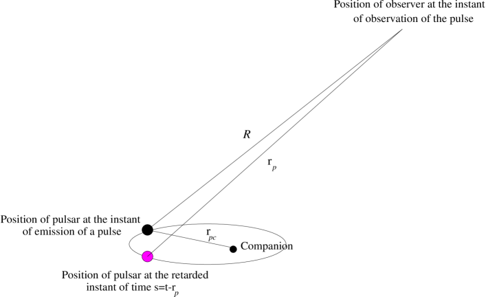
FIG. 2.: Schematic illustration of the Shapiro time delay in a binary pulsar. The pulsar emits radio signal at the time $t_{0}$ which reaches the observer at the time $t$. For calculation of the Shapiro time delay positions of the pulsar and its companion must be taken at the retarded instants of time $s_{0}$ and $s$ corresponding to those $t_{0}$ and $t$. See also Fig. 3 for further explanations.

FIG. 3.: Schematic space-time diagram showing the relationship between positions of a photon taken at different instants of time $t_{0}$, $t_{1}$,…, $t_{6}$ (events 0,1,…,6 on the photon’s null world line) and positions of the light-ray-deflecting bodies (marked by the black circles) taken at the instants of the retarded time corresponding to the instants $t_{0}$, $t_{1}$,…,$t_{6}$. For simplicity only the two-body system is considered. The photon is deflected by the retarded gravitational field of the bodies expressed through the Liénard-Wiechert potentials. Also shown are positions of the bodies (marked by the unfilled circles) taken on the space-like hypersurfaces (dashed lines) of the time instants $t_{0}$, $t_{1}$,…, $t_{6}$. As the photon approaches towards the system (events 0,1) it moves in the variable gravitational field of two bodies. After crossing the system (events 5,6) the gravitational field at the photon’s position is ”frozen” since the photon moves along the same light cone as the gravitational field propagates. The ”freezing” of gravitational field takes place during propagation of the photon inside the system (events 2,3,4). Spatial positions of gravitating bodies taken at the retarded instants of time are very close to those taken at the hypersurfaces of constant time when photon moves near or inside the system. It explains why the post-Newtonian solution for the metric tensor can be applied in this situation as well as the post-Minkowskian one for calculation of the photon’s propagation. Retarded and instanteneous spatial positions of the gravitating bodies are drastically different when photon is at large distance from the system (far outside the near zone). In this case only the post-Minkowskin retarded solution for the metric tensor can be applied for an adequate description of the gravitational perturbations of the photon’s trajectory.

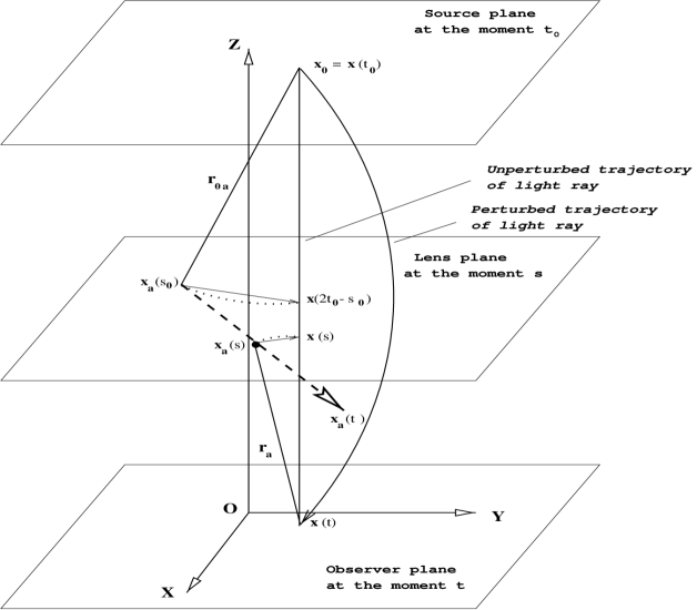
FIG. 4.: Relative configuration of observer, source of light and a moving gravitational lens deflecting light rays which are emitted at the moment $t_{0}$ at the point ${\bf x}_{0}$ and received at the moment $t$ at the point ${\bf x}$. The lens moves along straight line with constant velocity from the retarded position ${\bf x}_{a}(s_{0})$ through that ${\bf x}_{a}(s)$ and arrives to the point ${\bf x}_{a}(t)$ at the moment of observation. Characteristic time of the process corresponds to the time of propagation of light from the point of emission up to the point of observation.

FIG. 5.: The gravitational lens geometry for a moving lens ${\cal M}=\sum^{N}_{a=1}m_{a}$ being at the distance $r$ from the point of observation O with coordinates $x^{i}(t)$. A source of light S with coordinates $x_{0}(t_{0})$ is at the distance $R$ from O. Vector $\xi$ is the impact parameter of the unperturbed path of photon in the observer plane. Vector ${{\mbox{\boldmath$\xi$}}}_{L}$ denotes position of the center of mass of the lensing object in the lens plane. Vector ${{\mbox{\boldmath$\eta$}}}=\vec{BE}$ is the observed image position of the background source of light S shifted in the lens plane from its true position by the gravitational field of the lens to the point E. Coordinates of the lens are $X^{i}(\lambda^{\ast})={\cal M}^{-1}\sum^{N}_{a=1}m_{a}x_{a}^{i}(\lambda^{\ast})$, and coordinates of the point E are $x^{i}(\lambda^{\ast})=x^{i}(t)+s^{i}(\lambda^{\ast}-t)$.

FIG. 6.: Geodetic very long baseline interferometry measures delay $\tau$ (the light travel time between points 2 and 3) in times of arrival of radio signal from a quasar at the first and second radio antennas, $\tau=\tau_{2}-\tau_{1}$, located on the Earth’ surface. Diurnal rotation and orbital motion of the Earth makes the delay to be dependent on time. This allows to determine the baseline ${\bf b}$ between two antennas, astrometric coordinates of the quasar, motion of the Earth’s pole, parameters of precession and nutations, and many others. Modern data processing of VLBI observations is fully based on the relativistic conceptions and was supposed to be accurate up to 1 picosecond.

FIG. 7.: Spacecraft Doppler tracking experiment in deep space. Radio signal is transmitted at the time $t_{0}$ and at the point 0 on the Earth along the unit vector ${\bf k}_{1}$. The radio signal reaches the spacecraft at the moment $t_{1}$ and at the point 1 somewhere in the solar system and responds back to the Earth exactly at the same time $t_{1}$ along the unit vector ${\bf k}_{2}$ which has a different orientation from ${\bf k}_{1}$. The responded signal arrives at the reception point 2 on the Earth at the time $t_{2}$. During the round-trip time of the radio signal the Earth rotates around its own axis and moves along the orbit. Hence, the barycentric position and velocity of the transmitter is different from the barycentric position and velocity of the receiver despite of that their topocentric positions on the Earth can coincide. When the impact parameter of the radio signal’s trajectory is small the gravitational Doppler shift of the transmitted frequency with respect to the received frequency is estimated approximately as $\delta\nu/\nu_{2}=2\alpha(v_{\odot}/c)\cos\varphi$, where $\alpha$ is the deflection angle of the light ray, $v_{\odot}$ is velocity of the Earth, and $\varphi$ is the angle between $v_{\odot}$ and the impact parameter.