Relativistic hydrodynamics on spacelike and null surfaces: Formalism and computations of spherically symmetric spacetimes

Abstract

We introduce a formulation of Eulerian general relativistic hydrodynamics which is applicable for (perfect) fluid data prescribed on either spacelike or null hypersurfaces. Simple explicit expressions for the characteristic speeds and fields are derived in the general case. A complete implementation of the formalism is developed in the case of spherical symmetry. The algorithm is tested in a number of different situations, predisposing for a range of possible applications. We consider the Riemann problem for a polytropic gas, with initial data given on a retarded/advanced time slice of Minkowski spacetime. We compute perfect fluid accretion onto a Schwarzschild black hole spacetime using ingoing null Eddington-Finkelstein coordinates. Tests of fluid evolution on dynamic background include constant density and TOV stars sliced along the radial null cones. Finally, we consider the accretion of self-gravitating matter onto a central black hole and the ensuing increase in the mass of the black hole horizon.

I Introduction

The theoretical understanding of the detailed dynamics of black hole interactions with matter is today a key research activity, both in the gravitational wave [4] and high-energy astrophysics [5] communities. Such research targets the interpretation of data obtained (or anticipated) in a number of distinct observational windows, from high resolution spectra of regions suspected of harboring black holes, e.g., with satellite experiments like the Rossi X-ray Timing Explorer (RXTE) [2], to broad band gravitational wave detection efforts, e.g., the Laser Interferometric Gravitational Observatory (LIGO) [3]. Computations within the Newtonian paradigm have reached high levels of sophistication (see, e.g., [6]), offering important clues and support for further development of astrophysical models. Clearly, computations within the framework of general relativity would be highly desirable. Several efforts are underway for meeting the difficult challenge of solving the Einstein equations in full generality (e.g., [7, 8, 9, 10, 11]).

Yet the task before the computational scientists is daunting, as the underlying theory is rich in conceptual and technical complications. This attribute of relativistic gravity, led in the pre-60’s period to a certain confusion with respect to the physical content of the theory, e.g., as to whether gravitational waves exist at all. The conundrum was finally resolved with the introduction and masterly manipulation of the characteristic initial value problem (CIVP) by Bondi and Sachs [12, 13]. Important features of the CIVP suggest it may be serve as a valuable tool in the effort of studying interesting black hole spacetimes (a review of the development of algorithms based on the CIVP is given in [14]). We highlight, in particular, the long term stability of non-linear numerical evolution schemes based on null coordinates, shown for regular spacetimes in axisymmetry [15], and black hole spacetimes in full 3D [16]. Additionally, the schemes are of low computational cost per spacetime point, an issue which acquires significance when stability problems are controlled. Both features ultimately derive from the gauge properties of the null foliation, which captures directly the wave degrees of freedom as a propagation equation for a complex function, with all other relevant equations converted into ODE’s to be integrated along the characteristic surface. The CIVP formulation of the Einstein equations hence offers, with the inclusion of appropriate matter dynamics (e.g., in the form of perfect fluid hydrodynamics), among others, the possibility of accurate studies of generic black-hole-matter interactions.

The aim of this paper is to present and test a general formulation of the general relativistic hydrodynamic (GRH) equations for ideal fluids, appropriate for numerical work, which is suited, but not restricted, to integration on spacetimes foliated with null hypersurfaces. The form invariance of the approach with respect to the nature of the foliation implies that existing work on highly specialized techniques for fluid dynamics can be adopted with minimal modifications. In our program of studying black hole matter interactions we have already used such techniques in estimating gravitational radiation from bulk fluid accretion [17] in the black hole perturbation limit. The developments here constitute a first step in extending that program into the fully non-linear regime.

The paper contains four main sections. Section II presents the essential formal elements of a new prescription for solving GRH, i.e., a choice of conserved and primitive variables and their relationship, along with a diagonalization of the Jacobian matrix and explicit expressions for its eigenvalues and eigenvectors. In Section III we formulate the problem of coupled evolution of matter and geometry fields in spherical symmetry. The analog of the Tolman-Oppenheimer-Volkoff (TOV) equation is constructed and integrated along the null cone. Those solutions are used for consistency and convergence tests. Those are demonstrated, along with some relevant details of the numerical implementation, in Section IV. That Section also discusses the important issue of shock-capturing, explored for fluid data posed on a null surface (in flat spacetime). In Section V we turn to black hole spacetimes and spherical accretion. The test fluid limit is used as a test-bed, and we proceed to a preliminary study of self gravitating accretion.

We use geometrized units ($G=c=1$) and the metric conventions of [18]. Boldface letters (and capital indices) denote vectors (and their components) in the fluid state space.

II Formalism for general relativistic hydrodynamics

A Prelude to the formal developments

The traditional approach for relativistic hydrodynamics on spacelike hypersurfaces is based on Wilson’s pioneering work [19]. In this formalism the equations were originally written as a set of advection equations. This approach sidesteps an important guideline for the formulation of non-linear hyperbolic systems of equations, namely the preservation of their conservation form. This feature is necessary to guarantee correct evolution in regions of sharp entropy generation. Nevertheless, in the absence of such features, non-conservative formulations are equivalent to conservative ones. The approach is then simpler to implement and has been widely used over the years in a number of astrophysical scenarios. On the other hand, a numerical scheme in conservation form allows for shock-capturing, i.e., it guarantees the correct Rankine-Hugoniot (jump) conditions across discontinuities. Writing the relativistic hydrodynamic equations as a system of conservation laws, identifying the suitable vector of unknowns and building up an approximate Riemann solver has permitted the extension of modern high-resolution shock-capturing (HRSC in the following) schemes from classical fluid dynamics into the realm of relativity [20]. The main theoretical ingredients to construct such a scheme in full general relativity can be found in [21]. An up-to-date collection of different applications of HRSC schemes in relativistic hydrodynamics is presented in [22]. We will return to these schemes in section IV below.

Non finite-difference methods have also been applied recently to compute relativistic flows, most notably, pseudo-spectral methods and smoothed particle hydrodynamics (SPH) techniques. Although pseudo-spectral methods have enhanced accuracy in smooth regions of the solution, the correct modeling of discontinuous solutions is still their main drawback [23]. Recently, however, progress has been achieved in this direction by using multi-domain decomposition techniques [24]. On the other hand, SPH, as any other particle method, suffers from being dissipative when resolving steep gradients [25]. In spite of this, it has recently proven to work in the ultra-relativistic regime [26]. Additionally, it has been shown that it is possible to generalize SPH methods to hyperbolic systems other than the Euler equations [27]

Procedures for integrating various forms of the hydrodynamic equations on null hypersurfaces have been presented before [28] (see [29] for a recent implementation). This approach is geared towards smooth isentropic flows. A Lagrangian method, applicable in spherical symmetry, has been presented by [30]. Recent work in [31] includes an Eulerian, non-conservative, formulation for general fluids in null hypersurfaces and spherical symmetry, including their matching to a spacelike section. Here we show that the GRH equations can be formulated in a conservative and form invariant way (i.e., irrespective of the spacelike or null nature of the foliation) for an arbitrary three dimensional spacetime and any perfect fluid with polytropic equation of state.

B The formulation

1 Variables and evolution equations

We consider the relativistic conservation equations (continuity equation and Bianchi identities) upon introducing an explicit coordinate chart $(x^{0},x^{i})$, i.e.,

$$\frac{\partial}{\partial x^{\mu}}\sqrt{-g}J^{\mu} = 0\,,$$ (1)

$$\frac{\partial}{\partial x^{\mu}}\sqrt{-g}T^{\mu\nu} = -\sqrt{-g}\Gamma^{\nu}_{\mu\lambda}T^{\mu\lambda}\,,$$ (2)

where the scalar $x^{0}$ represents a foliation of the spacetime with hypersurfaces (coordinatized by $(x^{1},x^{2},x^{3})$), with the matter current and stress energy tensor for a perfect fluid given by $J^{\mu}=\rho u^{\mu}$, $T^{\mu\nu}=\rho hu^{\mu}u^{\nu}+pg^{\mu\nu}$, where $p$ is the pressure, $u^{\mu}$ is the fluid four velocity and $h=1+\varepsilon+p/\rho$ is the relativistic specific enthalpy.

We do not restrict the foliation to be spacelike (that is, the level surfaces of $x^{0}$ may be also null). We define the coordinate components of the four-velocity $u^{\mu}=(u^{0},u^{i})$. The velocity components $u^{i}$, together with the rest-frame density and internal energy, $\rho$ and $\varepsilon$, provide a unique description of the state of the fluid and will be called (following common usage) the primitive variables. They constitute a vector in a five dimensional space ${\bf w}^{A}=(\rho,u^{i},\varepsilon)$. The index $A$ is taken to run from zero to four, coinciding for the values (1,2,3) with the coordinate index $i$. We define the initial value problem for equations (1,2) in terms of another vector in the same fluid state space, namely the conserved variables, ${\bf U}^{B}$, individually denoted $(D,S^{i},E)$ [32],

$$D = {\bf U}^{0}=J^{0}=\rho u^{0}\,,$$ (3)

$$S^{i} = {\bf U}^{i}=T^{0i}=\rho hu^{0}u^{i}+pg^{0i}\,,$$ (4)

$$E = {\bf U}^{4}=T^{00}=\rho hu^{0}u^{0}+pg^{00}\,.$$ (5)

With those definitions the equations will take the standard conservation law form[33],

$$\partial_{x^{0}}(\sqrt{-g}{\bf U}^{A})+\partial_{x^{j}}(\sqrt{-g}{\bf F}^{jA})={\bf S}^{A}\,,$$ (6)

where $\sqrt{-g}$ is the volume element associated with the four-metric and we defined the flux vectors ${\bf F}^{jA}$ and the source terms ${\bf S}^{A}$ (which depend only on the metric, its derivatives and the undifferentiated stress energy tensor),

$${\bf F}^{j0} = J^{j}=\rho u^{j}\,,$$ (7)

$${\bf F}^{ji} = T^{ji}=\rho hu^{i}u^{j}+pg^{ij}\,,$$ (8)

$${\bf F}^{j4} = T^{j0}=\rho hu^{0}u^{j}+pg^{0j}\,,$$ (9)

$${\bf S}^{0} = 0\,,$$ (11)

$${\bf S}^{i} = -\sqrt{-g}\,\Gamma^{i}_{\mu\lambda}T^{\mu\lambda}\,,$$ (12)

$${\bf S}^{4} = -\sqrt{-g}\,\Gamma^{0}_{\mu\lambda}T^{\mu\lambda}\,.$$ (13)

The state of the fluid is uniquely described using either vector of variables, i.e., ${\bf U}^{A}$ or ${\bf w}^{A}$, and one can be obtained from the other, as will be shown later, via the definitions (3)-(5) and the use of the normalization condition for the velocity vector,

$$g_{\mu\nu}u^{\mu}u^{\nu}=-1\,.$$ (14)

Specification of ${\bf U}^{A}$ on the initial hypersurface, together with an equation of state (EOS) $p=p(\rho,\varepsilon)$, followed by a recovery of the primitive variables leads to the computation of the fluxes and source terms. Hence, the first time derivative of the data is obtained, which then leads to the formal propagation of the solution forward in time. No continuity of the data is required, since in practice the evolution is achieved with the (possibly approximate) solution of local Riemann problems.

2 Local characteristic structure of the equations

Utilizing the machinery of modern hydrodynamical methods, i.e., HRSC schemes, to integrate the previous equations requires the investigation of their local characteristic structure. We proceed here with this analysis. For this purpose we temporarily ignore the inhomogeneous part of the system.

Introducing the Jacobian matrices

$${\bf B}^{jA}_{B}=\frac{\partial{\bf F}^{jA}}{\partial{\bf U}^{B}}\,,$$ (15)

the system can be written in quasi-linear form as

$$\partial_{x^{0}}{\bf U}^{A}+{\bf B}^{jA}_{B}\partial_{x^{j}}{\bf U}^{B}=0\,.$$ (16)

The characteristic speeds (eigenvalues) and eigenvectors of the system, in the $j$-th direction, are then given by the solution of the algebraic problems (we now omit the vector indices of the fluid space)

$$det({\bf B}^{j}-\lambda^{j}{\bf I})=0\,,$$ (17)

$$({\bf B}^{j}-\lambda^{j}{\bf I}){\bf r}^{j}=0\,,$$ (18)

where $\lambda^{j}$ denotes the characteristic speed in the direction $j$, ${\bf r}^{j}$ the corresponding eigenvector and ${\bf I}$ denotes the unit matrix.

The strong coupling of the elements of the ${\bf B}$ matrix via the normalization condition hinders the analysis of the eigenvalue problem in terms of the conserved variables ${\bf U}$. The customary method to proceed (see [34]), is to analyze the problem in terms of the primitive variables. Indeed, the suitable choice of the primitive variables, such that the eigenvalue problem may be solved explicitly, is of great practical value.

With a choice of primitive variables ${\bf w}$, the quasi-linear system (16) is rewritten as

$${\bf A}^{0}\partial_{x^{0}}{\bf w}+{\bf A}^{j}\partial_{x^{j}}{\bf w}=0\,,$$ (19)

where

$${\bf A}^{0} = \frac{\partial{\bf U}}{\partial{\bf w}}\,,$$ (20)

$${\bf A}^{j} = \frac{\partial{\bf F}^{j}}{\partial{\bf w}}\,.$$ (21)

Hence, upon analyzing the algebraic system

$$det({\bf A}^{j}-\bar{\lambda}^{j}{\bf A}^{0})=0\,,$$ (22)

$$({\bf A}^{j}-\bar{\lambda}^{j}{\bf A}^{0})\bar{{\bf r}}^{j}=0\,,$$ (23)

elementary algebra establishes that $\bar{\lambda}^{j}=\lambda^{j}$ and the eigenvectors of matrix ${\bf B}^{j}$ are given by $\bar{{\bf r}}^{j}={\bf A}^{0}{\bf r}^{j}$.

We now proceed to diagonalize our system, with the choice of primitive variables ${\bf w}^{B}=(\rho,u^{i},\varepsilon)$, and specializing the derivation to the case of a perfect fluid EOS, $p=(\Gamma-1)\rho\varepsilon$, with $\Gamma$ being the (constant) adiabatic index of the fluid. The procedure can be generalized to an arbitrary EOS and details will be given elsewhere.

The matrices ${\bf A}$ are in this case

$\displaystyle{\bf A}^{0}=\left[\begin{array}[]{ccc}u^{0}&\rho\mu_{i}&0\\ hu^{0}u^{k}+(\Gamma-1)\varepsilon g^{0k}&\rho h(u^{0}\delta^{k}_{i}+u^{k}\mu_{i})&\rho\Gamma u^{0}u^{k}+(\Gamma-1)\rho g^{0k}\\ h(u^{0})^{2}+(\Gamma-1)\varepsilon g^{00}&2\rho hu^{0}\mu_{i}&\rho\Gamma(u^{0})^{2}+(\Gamma-1)\rho g^{00}\\ \end{array}\right]\,,$

$\displaystyle{\bf A}^{i}=\left[\begin{array}[]{ccc}u^{i}&\rho\delta^{i}_{j}&0\\ hu^{k}u^{i}+(\Gamma-1)\varepsilon g^{ki}&\rho h\delta^{k}_{j}u^{i}+\rho hu^{k}\delta^{i}_{j}&\rho\Gamma u^{k}u^{i}+(\Gamma-1)\rho g^{ki}\\ hu^{0}u^{i}+(\Gamma-1)\varepsilon g^{0i}&\rho hu^{0}\delta^{i}_{j}+\rho hu^{i}\mu_{j}&\rho\Gamma u^{0}u^{i}+(\Gamma-1)\rho g^{0i}\\ \end{array}\right]\,,$

with $\mu_{i}\equiv\frac{\partial u^{0}}{\partial u^{i}}=-\frac{u_{i}}{u_{0}}$. For a given coordinate direction, which we label ‘1’ (e.g., the $x^{1}$ direction), the matrix ${\bf A}^{1}-\lambda^{1}{\bf A}^{0}$ reads

$\displaystyle{\bf A}^{1}-\lambda^{1}{\bf A}^{0}=\left[\begin{array}[]{ccc}a&\rho b_{i}&0\\ hu^{k}a+(\Gamma-1)\varepsilon c^{k}&\rho h\delta^{k}_{i}a+\rho hu^{k}b_{i}&\rho\Gamma u^{k}a+(\Gamma-1)\rho c^{k}\\ hu^{0}a+(\Gamma-1)\varepsilon d&\rho hu^{0}b_{i}+\rho ha\mu_{i}&\rho\Gamma u^{0}a+(\Gamma-1)\rho d\\ \end{array}\right]\,,$

where the following shorthand notation is used

$$a \equiv u^{1}-\lambda^{1}u^{0},\hskip 32.72049ptb_{i}\equiv\delta^{1}_{i}-\lambda^{1}\mu_{i}$$ (24)

$$c^{k} \equiv g^{k1}-\lambda^{1}g^{0k},\hskip 28.45274ptd\equiv g^{01}-\lambda^{1}g^{00}.$$ (25)

The eigenvalues of that matrix are

$$\lambda^{1}_{0}=\frac{u^{1}}{u^{0}}\mbox{\,\,\,\,(triple)}\,,$$ (26)

and

$$\lambda^{1}_{\pm} = \frac{1}{1-c_{s}^{2}(1-{\cal L})}\left[{\cal M}c_{s}^{2}+v^{1}(1-c_{s}^{2})\mp c_{s}\sqrt{c_{s}^{2}{\cal M}^{2}+v^{1}(1-c_{s}^{2})(2{\cal M}-{\cal L}v^{1})+{\cal N}(1-c_{s}^{2}(1-{\cal L}))}\right]\,,$$ (27)

where all the metric information is encoded in the expressions ${\cal L},{\cal M}$ and ${\cal N}$,

$${\cal L} \equiv -\frac{g^{00}}{(u^{0})^{2}},\,\hskip 28.45274pt{\cal M}\equiv-\frac{g^{01}}{(u^{0})^{2}},\,\hskip 28.45274pt{\cal N}\equiv\frac{g^{11}}{(u^{0})^{2}}.$$ (28)

Additionally, $v^{1}\equiv\frac{u^{1}}{u^{0}}$ and $c_{s}$ is the local sound speed satisfying

$$hc^{2}_{s}=\chi+\frac{p}{\rho^{2}}\kappa\,,$$ (29)

with $\chi=\frac{\partial p}{\partial\rho}=(\Gamma-1)\varepsilon$ and $\kappa=\frac{\partial p}{\partial\varepsilon}=(\Gamma-1)\rho$. A complete set of right-eigenvectors is given by

$${\bf r}_{0,1}=u^{0}(1,u^{1},u^{2},u^{3},u^{0})\,,$$ (30)

$${\bf r}_{0,2}=(u^{0}+\rho\mu_{32},u^{0}u^{1}+\rho hu^{1}\mu_{32},u^{0}u^{2}+\rho h(u^{2}\mu_{32}-u^{0}b_{3}),u^{0}u^{3}+\rho h(u^{3}\mu_{32}+u^{0}b_{2}),(u^{0})^{2}+2\rho hu^{0}\mu_{32})\,,$$ (31)

$${\bf r}_{0,3}=(u^{0}+\rho\mu_{23},u^{0}u^{1}+\rho hu^{1}\mu_{23},u^{0}u^{2}+\rho h(u^{2}\mu_{23}+u^{0}b_{3}),u^{0}u^{3}+\rho h(u^{3}\mu_{23}-u^{0}b_{2}),(u^{0})^{2}+2\rho hu^{0}\mu_{23})\,,$$ (32)

$\displaystyle{\bf r}_{\pm}=\left[\begin{array}[]{c}-\frac{\rho}{\varepsilon}u^{0}B+\frac{\rho\Gamma}{h}K\\ \\ -\frac{\rho}{\varepsilon}u^{0}Bu^{1}h+\rho\Gamma[A(u^{0}c^{1}-ag^{01})+u^{1}K]\\ \\ -\frac{\rho}{\varepsilon}u^{0}Bu^{2}h+\rho\Gamma[A(u^{0}c^{2}-ag^{02})+u^{2}K]\\ \\ -\frac{\rho}{\varepsilon}u^{0}Bu^{3}h+\rho\Gamma[A(u^{0}c^{3}-ag^{03})+u^{3}K]\\ \\ -\frac{\rho}{\varepsilon}(u^{0})^{2}{\tilde{B}}+\rho\Gamma[2u^{0}K-aAg^{00}]\\ \end{array}\right]\,,$

with the definitions

$$A \equiv \frac{u^{0}-u^{i}\mu_{i}}{d-c^{i}\mu_{i}},\hskip 31.2982pt{\tilde{A}}\equiv\frac{\Gamma aA}{\Gamma-1},$$ (33)

$$B \equiv 1+{\tilde{A}},\hskip 48.36958pt{\tilde{B}}\equiv 1+h{\tilde{A}},$$ (34)

$$K \equiv \mu_{i}(Ac^{i}-u^{i}),\hskip 14.22636pt\mu_{ij}\equiv\mu_{i}b_{j}-\mu_{j}b_{i}.$$ (35)

Note that the $\pm$ dichotomy in the last two eigenvectors is implicit in the corresponding non-degenerate ($\pm$) eigenvalues through the variables $a$, $c^{i}$ and $d$.

The spectral decomposition given above applies to a chosen direction $j$. Since $j$ is arbitrary, to obtain similar expressions for the remaining directions, it suffices to specialize them accordingly, e.g., obtain the eigenvalues from expressions (26) and (27) with substitution of the desired direction, and permutation of the corresponding eigenvectors.

3 Relations between variables

So far the developments have been completely general. We specialize here the discussion to null coordinate systems.

For the EOS commonly accepted, the propagation speeds of fluid signals are always sub-luminal. In addition, the bulk flow is always assumed to be a timelike vector field. Hence, the Cauchy initial value problem for the fluid is well defined for data given on a null hypersurface (see Fig. 1).

While the numerical algorithm updates the vector of conserved quantities ($D,S^{i},E$), we make extensive use of the primitive variables ($\rho,u^{i},\varepsilon$). Those would appear repeatedly in the solution procedure: in the characteristic fields, in the solution of the Riemann problem and in the computation of the numerical fluxes (see below). Hence, it is necessary to specify a procedure for recovering them from the conserved quantities. In the spacelike case the relation between the two sets of variables is implicit. An example of an iterative algorithm to recover the primitive variables in this situation can be found in [35]. In the null case, the procedure of connecting primitive and conserved variables turns out to be explicit for a polytropic EOS. This is a direct consequence of the condition $g^{00}=0$ which characterizes null foliations [13] and leads to algebraic simplifications in the normalization expression $g^{\mu\nu}u_{\mu}u_{\nu}=-1$.

Assuming, hence, a perfect fluid EOS, the internal energy, $\varepsilon$, can be directly obtained in terms of the conserved quantities as the positive solution to a binomial equation, more precisely

$$\varepsilon=\frac{\Lambda^{2}}{D^{2}+D\sqrt{D^{2}+\Gamma(2-\Gamma)\Lambda^{2}}}\,,$$ (36)

where

$$\Lambda^{2}=-D^{2}-g_{00}E^{2}-2g_{0i}S^{i}E-g_{ij}S^{i}S^{j}\,.$$ (37)

Once $\varepsilon$ is known the rest of the primitive variables follow, e.g., $h=1+\Gamma\varepsilon$, $\rho=D^{2}h/E$, and

$$u^{i}=\frac{S^{i}-pg^{0i}}{D(1+\Gamma\varepsilon)}\,.$$ (38)

Having an explicit relation between conserved and primitive quantities has an impact on the efficiency of the numerical code, as it eliminates an iterative process that is required, at least once per each spacetime point. It is however unavoidable for general, e.g., tabulated, EOS.

III Non-vacuum spherically symmetric spacetimes in the Tamburino-Winicour formalism

We consider here the general spherically symmetric spacetime, with perfect fluid matter, following the formalism of Tamburino-Winicour [43], with a minor extension to cover the case of a worldtube immersed in matter.

The Einstein equations sufficient for obtaining the spacetime development are grouped as

$$G_{vr} = \kappa T_{vr},$$ (39)

$$G_{rr} = \kappa T_{rr},$$ (40)

$$G_{vv}|_{\Gamma} = \kappa T_{vv}|_{\Gamma},$$ (41)

where the $v$ coordinate is defined by the level surfaces of a null scalar (i.e., a scalar $v$ satisfying $\nabla^{\mu}v\nabla_{\mu}v=0$). The $r$ coordinate is chosen to make the spheres of rotational symmetry have area $4\pi r^{2}$. The $x^{2},x^{3}$ coordinates in this geometry are simply taken to be the angular coordinates $(\theta,\phi)$ propagated along the generators of the null hypersurface, i.e., they parameterize the different light rays on the null cone. The first two equations contain only radial derivatives and are to be integrated along the null surface. The last equation (41) is a conservation condition to be imposed on the world-tube $\Gamma$ (see Fig. 1). Equation (40) may be substituted for by the equivalent expression $g^{ab}R_{ab}=8\pi g^{ab}(T_{ab}-g_{ab}T/2)$, where the indices $(a,b)$ run over the remaining coordinates $x^{2},x^{3}$. To proceed with the integration, an additional choice of gauge must be made on the worldtube. This condition fixes the only remaining freedom in the coordinate system, namely the rate of flow of coordinate time at the world-tube.

We present here the explicit expressions we use, including the matter terms. Adopting the Bondi-Sachs form of the metric element,

$$ds^{2}=-\frac{e^{2\beta}V}{r}dv^{2}+2e^{2\beta}dvdr+r^{2}(d\theta^{2}+\sin\theta^{2}d\phi^{2})\,,$$ (42)

the geometry is completely described by the two functions $\beta(v,r)$ and $V(v,r)$ (we will also interchangeably use the variable $W=V-r$).

The $\beta$ and $V$ hypersurface equations are given by

$$\beta_{,r} = 2\pi rT_{rr}\,,$$ (43)

$$V_{,r} = e^{2\beta}+4\pi rVT_{rr}+8\pi r^{2}T_{rv}\,,$$ (44)

the latter being equivalent (modulo the four-velocity normalization condition) to

$$V_{,r}=e^{2\beta}(1-4\pi r^{2}(g^{AB}T_{AB}-T))\,.$$ (45)

The comma in the above equations indicates, as usual, partial differentiation.

Boundary conditions $(\beta(v)_{\Gamma},V(v)_{\Gamma})$ for the radial integrations are provided by the equation (41) which explicitly reads,

$$\frac{V\beta_{,r}}{r}+\beta_{,v}-\frac{V_{,v}}{2V}-\frac{V_{,r}}{2r}+\frac{1}{2r}e^{2\beta}-4\pi\frac{r^{2}}{V}T_{vv}=0\,,$$ (46)

with the adoption of a suitable gauge condition. For each choice one obtains a pair of ODE’s along the worldtube. For example, with the choices

$$V_{,v} = -8\pi r^{2}T_{vv}\,,$$ (47)

$$V_{,v} = 0\,,$$ (48)

$$(Ve^{2\beta})_{,v} = 0\,,$$ (49)

one obtains

$$\beta_{,v} = 4\pi rT_{vr}\,,$$ (50)

$$\beta_{,v} = 4\pi rT_{vr}+4\pi r^{2}T_{vv}/V_{0}\,,$$ (51)

$$\beta_{,v} = 2\pi rT_{vr}-2\pi e^{2\beta}T_{vv}/g_{00}\,,$$ (52)

respectively, where $V_{0}$ and $g_{00}$ denote the integration constants at $v=0$. All the above conditions are equivalent in vacuum, and since our present computations place the worldtube in very low density regions, we do not analyze the issue further.

The hydrodynamic equations reduce, within our symmetry assumptions, to:

$$D_{,v}+F^{r0}_{,r} = -(\ln{\cal V})_{,v}D-(\ln{\cal V})_{,r}F^{r0}\,,$$ (53)

$$S^{r}_{,v}+F^{r1}_{,r} = -(\ln{\cal V})_{,v}S^{r}-(\ln{\cal V})_{,r}F^{r1}-\Gamma^{r}_{\mu\nu}T^{\mu\nu}\,,$$ (54)

$$E_{,v}+F^{r4}_{,r} = -(\ln{\cal V})_{,v}E-(\ln{\cal V})_{,r}F^{r4}-\Gamma^{v}_{\mu\nu}T^{\mu\nu}\,,$$ (55)

where ${\cal V}=\sqrt{-g}=r^{2}\sin\theta e^{2\beta}$ is the four dimensional volume element. The precise form of the flux terms is obtained with direct use of the general formulae (9) and the Christoffel symbols $\Gamma^{v}_{\mu\nu}$ are derived explicitly for metric (42).

In summary, the initial value problem consists of equations (43,44,47-55) together with initial and boundary data for the fluid variables $(\rho,\varepsilon,u^{r})$ on the initial slice $\Sigma_{0}$ (at time $v_{0}$) and the metric values of $\beta(v_{0})_{\Gamma}$ and $V(v_{0})_{\Gamma}$ at the woldtube. Those equations and initial data are sufficient for obtaining the spacetime in a domain to the future of the initial hypersurface, which is radially bounded by the worldtube.

A Stationary configurations: Tolman-Oppenheimer-Volkoff solutions along the null cone

We present here the equations describing a spherically symmetric equilibrium configuration in null coordinates. Such solutions constitute an excellent test-bed for consistency and accuracy checks of our algorithms. For the simplest derivation, it will be advantageous to use a slightly different form of the metric element. With the redefinition $Y=Ve^{-2\beta}$, it reads,

$$ds^{2}=-\frac{e^{4\beta}Y}{r}dv^{2}+2e^{2\beta}dvdr+r^{2}(d\theta^{2}+\sin\theta^{2}d\phi^{2})\,.$$ (56)

In analogy with the spacelike foliated case, the stationarity in all metric and fluid variables reduces the number of non-trivial equations to the following coupled pair,

$$p_{,r} = \left(\frac{1}{2r}-\frac{1}{2Y}(1+8\pi r^{2}p)\right)\rho h\,,$$ (57)

$$Y_{,r} = 1+8\pi r^{2}(p-\rho h)\,,$$ (58)

where it is easily recognized that equation (57) is the radial momentum balance equation (54). This system of equations is solved as a system of ODE’s.

In the special case of a “stellar configuration”, solutions are obtained by starting, e.g., with initial conditions $p=p_{c},Y=0$ at the center of the star and integrating outwards until the pressure crosses the zero level [44]. Following that recipe, the direct integration of Eq. (43), with the boundary condition $\beta=0$ at the origin, completes the metric element. Fields of a representative solution, which we use in the next section for code testing are presented in Fig. 2.

1 Constant density star

In special cases the TOV equations can be integrated explicitly in terms of simple functions. A widely known example is the constant density star ($\rho_{0}$), derived here in ingoing null coordinates,

$$\beta = \frac{1}{2}\ln{\frac{3A-B}{2B}}\,,$$ (59)

$$V = \frac{rB}{2}(3A-B)\,,$$ (60)

$$p = \rho_{0}\frac{B-A}{3A-B}\,,$$ (61)

where $A=\sqrt{1-2M/R}$, $B=\sqrt{1-2Mr^{2}/R^{3}}$ and $M=4\pi\rho_{0}R^{3}$, with $R$ being the radius of the star.

IV Algorithms and Tests

The general formalism outlined in the previous two sections can form the basis for a variety of numerical approaches. Concerning the GRH equations, in the original Wilson’s scheme [19], a combination of finite-difference upwind techniques with artificial viscosity terms were used to damp spurious oscillations, extending the classic treatment of shocks introduced by von Neumann (see, e.g., [36]) into the relativistic regime. Artificial viscosity based methods, though, were later shown to fail at the threshold of the ultra-relativistic regime, once the Lorenz factor exceeds a value of 2. Explicit HRSC codes, following the so-called “Godunov approach”, appeared as a much more solid alternative.

Since the early nineties, it has been gradually demonstrated (see, e.g., [21] and references therein), that methods exploiting the hyperbolic character of the hydrodynamic equations are optimally suited for accurate integrations, even well inside the ultra-relativistic regime. As mentioned previously, these schemes are commonly known as high-resolution shock-capturing schemes. In a HRSC scheme, the knowledge of the characteristic fields (eigenvalues) of the equations, together with the corresponding eigenvectors, allows for accurate integrations, by means of either exact or approximate Riemann solvers, along the fluid characteristics. These solvers, which constitute the kernel of our numerical algorithm, compute, at every interface of the numerical grid, the solution of local Riemann problems (i.e., the simplest initial value problem with discontinuous initial data). Hence, HRSC schemes automatically guarantee that physical discontinuities appearing in the solution, e.g., shock waves, are treated consistently (the shock-capturing property). HRSC schemes are also known for giving stable and sharp discrete shock profiles. They have also a high order of accuracy, typically second order or more, in smooth parts of the solution.

We proceed now to describe the highlights of our implementation. The grid structure is, in summary, as follows: An equidistant radial grid $r_{i}$, with spacing $\Delta r$, denotes the location of cell centers on which the conserved variables and metric element components reside. The interface locations $r_{i}^{I}=r_{i}-\Delta r/2$ are used for the reconstruction of variables and the solution of the Riemann problems. Appropriate number of ghost-zones are added on the boundaries of the grid to allow imposition of boundary conditions. In particular, the worldtube conditions (47-50) are discretized in time along the first ghost-zone at $r_{N+1}$, where $r_{N}$ denotes the last cell center inside the domain. The timestep is variable and consistently computed to satisfy the Courant condition for the hydrodynamic equations. The geometric equations, being ODE’s in spherical symmetry, do not impose any timestep restriction.

Our numerical implementation of the coupled system is broadly based on the notion of operator splitting, i.e., the integration of the initial value problem in steps, by successive applications of split components of the overall evolution operator. We describe here, schematically, the procedure. The set of equations, comprised of the three hydrodynamical equations in spherical symmetry, and the hypersurface equations governing the geometry, are written as

$$\partial_{v}{\bf U} + \partial_{r}{\bf F}({\bf w},{\bf G})=0\,,$$ (62)

$$\partial_{v}{\bf U} \hskip 49.79231pt={\bf S}_{U}({\bf w},{\bf G})\,,$$ (65)

$${\bf A}({\bf U},{\bf w},{\bf G})=0\,,$$

$$\partial_{r}{\bf G}\hskip 27.88358pt={\bf S}_{G}({\bf w},{\bf G})\,.$$

The ordering of the equations reflects the sequence in which they are solved in the code. We denote the metric variables collectively as ${\bf G}$, while ${\bf A}$ stands for the set of algebraic relations connecting conserved and primitive variables (with the mediation of the metric). The velocity normalization condition is included with this set.

The first step in the solution process involves an advection of the conserved variables ${\bf U}$, from the initial data hypersurface $\Sigma_{0}$ to the hypersurface $\Sigma_{\Delta v}$. The computation of the fluxes F uses the metric as it is given in $\Sigma_{0}$, along with the primitive variables that are assumed to have been computed on $\Sigma_{0}$ in the previous iteration. The advection may be performed by any modern numerical scheme for the propagation of non-linear waves, i.e., by any HRSC scheme. These schemes, being written in conservation form, are particularly well suited for this purpose. Hence, all conserved quantities in the differential equations are also conserved in their finite-differenced versions. More precisely, the time update of

$$\partial_{v}{\bf U}+\partial_{r}{\bf F}=0\,,$$ (66)

is done according to the following algorithm:

$${\bf U}_{i}^{n+1}={\bf U}_{i}^{n}-\frac{\Delta v}{\Delta r}(\widehat{{\bf F}}_{i+1/2}-\widehat{{\bf F}}_{i-1/2})\,.$$ (67)

The index $n$ represents the time level, while the time discretization interval is indicated by $\Delta v$. The “hat” in the fluxes is used to denote the so-called numerical fluxes which, in a HRSC scheme, are computed according to some generic flux-formula, of the following functional form:

$$\widehat{{\bf F}}_{i\pm{1\over 2}}=\frac{1}{2}\left({\bf F}({\bf U}_{i\pm{1\over 2}}^{L})+{\bf F}({\bf U}_{i\pm{1\over 2}}^{R})-\sum_{\alpha=1}^{p}\mid\widetilde{\lambda}_{\alpha}\mid\Delta\widetilde{\omega}_{\alpha}\widetilde{r}_{\alpha}\right)\,.$$ (68)

Notice that the numerical flux is computed at cell interfaces ($i\pm 1/2$). Indices $L$ and $R$ indicate the left and right sides of a given interface. The sum extends to $p$, the total number of equations. Finally, quantities $\lambda$, $\Delta\omega$ and $r$ denote the eigenvalues, the jump of the characteristic variables and the eigenvectors, respectively, computed at the cell interfaces according to some suitable average of the state vector variables.

In our code, the numerical integration of the hydrodynamic equations can be performed using two different approximate Riemann solvers. These are the Roe solver [37], widely employed in fluid dynamic simulations, with arithmetically averaged states (for the use of the Roe mean in a relativistic Roe solver see [38]) and the Marquina solver, recently proposed in [39] (see also [40]).

After the update of the transport terms the fluid variables are subsequently corrected for the effect of the source terms. Any stable ODE integrator is usable here. Our choice is a second order Runge-Kutta method. A point of interest here is that the source terms ${\bf S}_{U}$ depend on both fluid and metric variables, and, in particular, on time derivatives of the latter. This implies that a second order capturing of the effect of those derivatives requires storing an additional time level of metric variables.

The geometry equations comprise a system of radial ODE’s, in which the right-hand-side depends on both the metric and the stress-energy tensor, a system to be solved on the hypersurface $\Sigma_{\Delta v}$. Initial conditions are provided on the world-tube. Hence, the integration cannot proceed without the recovery of the primitive variables on $\Sigma_{\Delta v}$, using the expressions given in section II B 3. It can be seen that those expressions involve the metric (which is to be solved for). Furthermore, one must worry about the preservation of the velocity normalization condition, which strongly depends on the metric at a given point. This differential-algebraic entangling of metric and fluid variables, generic to any attempt to solve general fluid spacetimes using conservative formulations, is approached in the following way:

The ODE integrator for equation (65) is chosen to belong to the implicit class. Our present choice is the second order Euler method. The metric variables in the new radial location $r_{i+1}$ are obtained iteratively ($k$ denotes the iteration index). Inside the $k$-iteration loop the intermediate metric variables ${\bf G}_{i+1}^{k}$ are used to obtain intermediate primitive variables ${\bf w}_{i+1}^{k}$, which then leads to updated values for the source term ${\bf S}_{G,i+1}^{k}$. In addition, the zeroth component of the velocity vector is adjusted so that the primitive velocity field $u^{\mu}$ is normalized. This process can be described as

$${\bf A}({\bf U}_{i+1},{\bf w}_{i+1}^{k},{\bf G}_{i+1}^{k})=0\,,$$ (69)

$${\bf G}_{i+1}^{k}-{\bf G}_{i}=\frac{\Delta r}{2}({\bf S}_{G,i+1}^{k}+{\bf S}_{G,i})\,,$$ (70)

(the time level index has been suppressed here for clarity). In practice the number of required iterations is about four or five. The completion of this procedure furnishes simultaneously the metric and the primitive variables at the new radial location, at the new time level.

A The Riemann problem on a null Minkowski slice

We proceed now to establish the feasibility of our proposal by performing numerical integrations of the GRH equations on null surfaces. Using the characteristic fields derived previously, we show here with two numerical examples the capabilities of existing HRSC schemes to integrate discontinuous solutions described in characteristic spacetime foliations. The initial data are given on a null slice (advanced or retarded time) of Minkowski space, and the evolution is compared to the suitably transformed exact solution.

The shock tube (a particular case of the Riemann problem) is one of the standard tests to calibrate numerical schemes in classical fluid dynamics. The initial setup of this experiment consists of a zero velocity fluid having two different thermodynamical states on either side of an interface. When this interface is removed, the fluid evolves in such a way that four constant states occur. Each state is separated by one of three elementary waves: a shock wave, a contact discontinuity and a rarefaction wave. This time-dependent problem has an exact solution [41], to which the numerical integration can be compared. In addition, it provides a severe test of the shock-capturing properties of any numerical scheme. In recent years, the shock tube problem began being used as a test of (special) relativistic hydrodynamical codes (see, e.g., [40] and references therein). The analytic solution of the Riemann problem, also available in relativistic hydrodynamics since [42], allows for a rapid and unambiguous comparison with the numerical evolutions.

For our numerical demonstrations we consider two different initial setups. In case 1 the initial state of the fluid is specified by $p_{L}=13.3$, $\rho_{L}=10$ on the left side of the interface and $p_{R}=0$, $\rho_{R}=1$ on the right side. For numerical reasons, the pressure of the right state is set to a small finite value ($p_{R}=0.66\cdot 10^{-6}$). Case 2 is as case 1 but with the left and right states reversed. We use a perfect fluid EOS with $\Gamma=5/3$.

1 The advanced time case

In Fig. 3 we plot the results for case 1. The left panels show the whole domain, with the $x$-coordinate ranging from 0 to 1000. The right panels show a zoomed up view of the most interesting domain ($x\in[750,950]$). We use a numerical grid of 2000 zones and, hence, a rather coarse spatial resolution ($\Delta x=0.5$).

¿From top to bottom, Fig. 3 displays the internal energy ($\varepsilon$), the velocity ($u^{x}$) and the density ($\rho$). The thick dotted line represents the initial discontinuity. The solid line shows the exact solution after an advanced time $v=270$ and the dotted line indicates the numerical solution at this same time. In order to compute the exact solution in our new coordinates we have followed the procedure outlined in [42] applying the appropriate time transformation, i.e., $t=v-x$. Clearly, the agreement between the exact (solid lines) and numeric solution is remarkable. The solution is characterized by an (outgoing) shock wave (moving to the right) and an (ingoing) rarefaction wave (moving to the left). One important point to notice is that features of the solution moving towards the left are more developed than those moving to the right. This is visible in the respective locations of the head of the rarefaction and the shock wave with respect to the initial discontinuity. The appearance of the rarefaction wave differs from the standard “spacelike” one (see, e.g., Fig. 2 of [40]), due to the intervening time transformation. The internal energy and the density show an additional elementary wave, a contact discontinuity between the shock and rarefaction waves. Across the contact discontinuity pressure and velocity are constant, while the density exhibits a jump.

In the right panels we note that the largest discrepancies are found at the tail of the rarefaction, in the form of an “undershooting” in density and internal energy and an “overshooting” in velocity. This is a typical feature of the numerical solution of the shock tube problem and it is not related to the null coordinates used here. We note that the constant state between the shock wave and the contact discontinuity is well resolved despite the coarse resolution used. For comparison purposes, the interested reader is referred to [40], where similar results were obtained (in a spacelike approach) employing a grid resolution 200 times finer.

2 The retarded time case

In Fig. 4 the results for the “mirror” version of the shock tube problem 1 are plotted. As in Fig. 3, the left panels show the whole domain, with the $x$-coordinate ranging from 0 to 1000 whereas the right panels show a closed-up view of the most interesting region ($x\in[180,820]$). We use the same grid resolution as in case 1. The initial data are now evolved up to a final time $v=120$. Again, those features of the solution moving towards the left are more developed than those moving towards the right. The “tower” in the density is now considerably wider than in case 1 as well as the intermediate constant state in the internal energy between the shock and the contact discontinuity (almost not noticeable in case 1). This constant state is much more accurately resolved than in case 1 despite the use of the same resolution. The two corners of the rarefaction wave are also very well resolved. The major numerical deviations from the exact solution appear now at the post contact discontinuity region, with the density and the internal energy being slightly under and over estimated there.

We should comment on the different ways in which the shock is captured in cases 1 and 2. Whereas in case 1 the shock is spread out in a number of grid zones ($\approx 10$), in case 2 it is sharply resolved in 2-3 cells (out of the 2000 zones used). This is shown in Fig. 5. Those differences ultimately derive from the fact that a retarded (or advanced) time formulation of a Riemann problem (assuming, for the discussion, the initial discontinuity located at $x=0$) breaks the commutation between the operation of reflection symmetry (between positive and negative values of $x$) and that of time evolution. The significance of this effect in applications involving shocks and its possible exploitation for ultrarelativistic outflows will be studied elsewhere.

We also include in Fig. 6 the evolution of the outgoing shock of case 1 at two different times, $v=300$ and $v=600$. For this run we are using $4000$ zones with the $x$-coordinate ranging from 0 to 2000. Hence, the spatial resolution is again $\Delta x=0.5$. The initial discontinuity is placed at $x=1650$. The solution was left to evolve for a time considerably longer than before in order to find out if the numerical representation of the shock had more time to accommodate itself into a sharper profile. From Fig. 6 we find this not to be the case. The initial spreading present in the numerical solution remains constant in time. It is noteworthy to mention the independence of the number of points in which the shock is resolved from the total number of zones used.

B Convergence testing of the coupled code

The TOV solutions presented before constitute a good test-bed for confirming both the consistency and the accuracy of the algorithm. The availability of semi-analytic solutions to the stationary problem means that there is a host of error functions that can be constructed by subtracting the evolved solution at a fixed total time $t_{F}$ from the initial profile. As an example, using the exact density profile $\rho_{E}$, the quantity

$$\|\rho-\rho_{E}\|_{2}=\sum_{i}(\rho_{i}-\rho_{E})^{2}$$ (71)

measures the deviations produced by the numerical evolution.

As our present implementations are geared towards black hole spacetimes (with topology of $S^{2}\times R$ rather than regular $R^{3}$ spacetimes), in order to benefit from this test-bed without undue boundary complications, we consider only a portion of the spacetime, excluding the domain around $r=0$. Initial data for the fluid and the metric are obtained with the solution of the TOV equations along the past null-cone of the center of symmetry. The integration then proceeds in the regular fashion described above, but restricted to a domain inside the star, e.g., in the sample shown in Fig. 2 this extends between $r=2$ and $r=6$. In the plots given in Fig. 7 we consider the convergence of such functions and their $L_{2}$ norms to zero, as the grid spacing is reduced. The norm is found to converge to third order. This can be seen in the insert of Fig. 7, where the final values of the norm at $v=40$ (about eight light crossing times) are plotted against grid size. This implies that the local error is second order.

The constant density solution is obtained with the assumption of an ad-hoc (and largely unphysical) equation of state and hence it is not possible to evolve such data with the formalism developed here, but it is straightforward to test the integration of the hypersurface equations against the exact solution. We have confirmed that the integrated metric agrees along the hypersurface with the exact value to second order in the radial grid spacing.

V Spherical accretion onto a black hole

We proceed now in applying the formalism, in spherical symmetry, to the problem of interaction of matter with a black hole. In recent work [45] the interaction of a scalar field with a black hole was investigated, partly as a probe into the concept of “singularity excision” [46, 47, 48]. Following that same concept in spirit, in a previous investigation, we studied fluid interactions with the black hole geometry, in the test-fluid limit. We dubbed stationary coordinates that are regular at the horizon of an exact stationary black hole solution as horizon adapted coordinate systems [49]. In those coordinates the flow solution is smooth and regular at the black hole horizon. The steepness of the hydrodynamic quantities dominates the solution only near the real singularity. This approach is now being applied in successively more general (and astrophysically interesting) fluid configurations [50, 51]. We extend here this line of work by first performing test-fluid computations in the spirit of [49] for the null Eddington-Finkelstein coordinate system. This is next further generalized to account for self-gravitating accretion flows.

A The test fluid limit

We study spherical accretion of a perfect fluid onto a (static) black hole. The fluid is taken to have a sufficiently low density so that during the accretion process the mass of the black hole remains unchanged. Stationary solutions to this idealized problem can be computed exactly, up to algebraic equations. This was first derived for Newtonian flows by Bondi [52]. The extension to general relativity was due to Michel [53]. The solution can easily be re-derived for coordinates other than the original Schwarzschild system employed by Michel (the details can be found in [49]). We use next this exact solution to quantify the accuracy of our numerical integrations. The significance of the test lies in its capturing of large curvature gradients near the black hole (i.e., it is a strong field computation), which translates into the existence of large source terms in the hydrodynamic equations.

We use ingoing Eddington-Finkelstein $(v,r,\theta,\phi)$ coordinates for which the line element reads

$$ds^{2}=-\left(1-\frac{2M}{r}\right)dv^{2}+2dvdr+r^{2}(d\theta^{2}+\sin^{2}\theta d\phi^{2})\,,$$ (72)

where $M$ is the mass of the black hole. The expressions for the characteristic fields of the hydrodynamic equations are then specialized using the above metric components. We use a polytropic EOS with $\Gamma$ (the adiabatic exponent of the gas) equal to $5/3$. The numerical domain extends from any given non-zero radius inside the horizon, $r_{min}$, to some outer radius $r_{max}$ (outside and far from the black hole horizon). In the particular simulation reported here we choose $r_{min}=1.5M$ (inside the black hole horizon, located at $r=2M$) and $r_{max}=30M$. We use a uniform (equally spaced) numerical grid of 200 zones.

The test proceeds as follows: We set the semi-analytic solution as initial data throughout the domain, and then evolve these data, maintaining the exact solution as a constant inflow boundary condition at the outer boundary. Representative results are summarized in Figs. 8-10.

In Figure 8 we display only the solution up to a radius of $10M$, in order to focus on the most interesting, strong field region, around the black hole horizon. The figure displays the primitive variables, ($\rho,u^{r},\varepsilon$), as functions of the ingoing Eddington-Finkelstein radial coordinate. These figures show the capturing of the steady-state spherical accretion solution. The solid lines represent the exact solution, while the filled circles indicate the numerical one. The latter has been evolved up to a time $v=500M$. The agreement between the exact and numerical solutions is very good for all fields. This is more clearly seen in Fig. 9 where we plot the relative errors of the primitive variables. The largest errors appear at the innermost zones. The maximum error never exceeds 2%, for the internal energy, or 1%, for the density, even with the relatively coarse grid of 200 points. The quality of the results for the velocity is excellent, with the maximum relative error being about 0.1%.

In Fig. 10 the convergence properties are captured more quantitatively. The squared difference of the density from the exact result, integrated over the entire domain (the $L_{2}$ norm), is plotted as a function of advanced time, for a total time of 200. After an initial rise, the error settles into a final state, the level of which is converging to third order with the radial grid size.

We note in passing that no secular instabilities of any kind arise during the computation, for total number of iterations of the order of $10^{5}$. Besides the intrinsic value of the test as an exact strong field solution, an important practical aspect merits mentioning here: very low density spherical inflow solutions constitute a good background flow, useful in computations where the primary dynamics of interest involves high density concentrations around the black hole.

B Accretion of a self-gravitating perfect fluid

In our last numerical demonstration we investigate the accretion of a self-gravitating perfect fluid onto a non-rotating black hole. The setup of the simulation is as follows: Boundary values corresponding to a black hole of given mass $M_{F}$ are specified at the world-tube, located at $r_{B}$. The interior to that radius is filled first with low density data which do not interact with the black hole geometry in the timescales of interest. The dynamically interesting fluid component, typically a high density distribution (compared to the background) of compact support with sufficiently strong self-gravity, is added next. The data to be specified are $(\rho,\epsilon,u^{r})$ and are, in short, completely arbitrary, with one exception: For the setup to correspond to a spacetime with a trapped region, i.e., with a horizon, the added fluid mass should not exceed $M_{F}$. The velocity profile is borrowed from the Bondi accretion solution and, hence, corresponds to an inwards monotonically increasing velocity. The initial data for the density are specified with explicit profiles, e.g., flat or Gaussian radial distributions. In our simulations we consider a Gaussian spherical shell surrounding the central black hole, with density parameterized according to

$$\rho=\rho_{b}+\rho_{m}e^{-\sigma(r-r_{c})^{2}}$$ (73)

where $\rho_{b}$ is the background density. The rest of parameters take the values: $\rho_{m}=10^{-4}$, $\sigma=0.1$ and $r_{c}=6M$. The grid extends from $r_{min}=1.1M$ to $r_{max}=20M$. Finally, the internal energy is obtained assuming an initially isentropic distribution of pressure $p=K\rho^{\Gamma}$ (which would be valid at later times only for equilibrium configurations).

The results of the simulation are plotted in Figs. 11, 12 and 13. In Fig. 11 we display the evolution of the primitive variables $(\rho,u^{r},\epsilon)$, from top to bottom, as a function of the ingoing Eddington-Finkelstein radial coordinate, $r$. The configuration is radially advected (accreted) towards the hole in the first $10M-15M$. Once the bulk of the accretion process ends, we are left with a quasi-stationary background solution (basically equivalent to the Bondi solution). In Fig. 12 we plot the evolution of the logarithm of the Riemann scalar curvature. We note that the initial shell has associated with it a non-negligible curvature. At late times the solution is again dominated by the curvature of the central black hole.

The location of the apparent horizon of the black hole can be easily computed during the evolution. For the simplified case of spherical symmetry, this location is just given by the zero of the $g_{00}$ metric component. Our results show that the accretion process initiates a rapid increase of the mass of the apparent horizon. This is depicted in Fig. 13. The horizon almost doubles its size during the first $10M-15M$ (this is enlarged in the insert of Fig. 13). Once the main accretion process has finished, the mass of the horizon slowly increases, in a quasi-steady manner, whose rate depends on the mass accretion rate imposed at the world-tube, $\Gamma$, of the integration domain. The numerical solution can be evolved as far as desired into the future.

VI Summary and Conclusions

The equations of general relativistic hydrodynamics have been written directly in terms of components of the fluid fields in an arbitrary coordinate patch. The system of equations has been diagonalized in the general case, aiming at the subsequent use of advanced numerical methodology. The conservation form of the equations is preserved to the degree possible, whereas the formulation does not require a spacelike foliation for its implementation.

We may ask whether there is any unexpected element in the developments here. The formulation of the hydrodynamic equations as a Cauchy problem, (well) posed on a null spacetime surface, is intuitively expected and has been formulated before as mentioned in the text. The writing of the equations as a system of conservation laws on an arbitrary foliation is implicit in their abstract representation. It is further expected that for any non-degenerate choice of primitive fields, the system will be hyperbolic and diagonalizable. What does appear to be more of a happy algebraic coincidence rather than a general feature is the possibility of explicitly solving for the eigenfields. Indeed, choices of variables close to the ones presented here do not allow explicit diagonalization. We are aware of two cases in the literature where similar explicit resolutions as the ones reported here have been achieved. In the first case the authors made an explicit assumption of a spacelike foliation [21] (see also [9]), while the second [38] appears motivated by a choice of variables specific to a non-relativistic Riemann solver (the Roe solver), and leads to expressions considerably more complicated than the ones presented here.

We have developed a number of test-beds by recomputing known solutions in our coordinates. The performance of the algorithm was satisfactory in each instance, which establishes the overall feasibility of the approach. The practical value of this demonstration is that advanced schemes developed for the hydrodynamic equations by a large community of researchers (encompassing computational astrophysics) will be available with minimal modifications to this more specialized field. A further point of interest is that it is demonstrated here, implicitly, that the Newtonian pedigree of the field of hydrodynamics is essentially bypassed in the formulation of the relativistic equations as conservation laws. Our variables have no connection, in the null case, to the instantaneous rest frame (Eulerian) observers defined by the normal to a spacelike hypersurface.

The selection of computations in the last section is geared towards highlighting the suitability of our approach to the study of black holes interacting with matter. In a representative computation, we have shown how a non-trivial increase of the mass of the black hole horizon can be achieved naturally in the present framework. This can be contrasted with the considerably harder task of achieving long term black hole evolutions in a spacelike approach, as it is seen, for example, in [54].

Extending the present setup to three-dimensional spacetimes appears to be an important target for the near future. In this respect, the feasibility of extending the vacuum CIVP with the inclusion of matter sources has recently been reported [29].

VII Acknowledgments

We thank Ed Seidel for supporting this project since its inception and José M${}^{\underline{\mbox{a}}}$. Ibáñez for many useful discussions. Most computations were performed at the Origin 2000 supercomputer of the AEI. P.P would like to thank SISSA for hospitality while parts of this work were being completed. J.A.F acknowledges financial support from a TMR grant from the European Union (contract nr. ERBFMBICT971902).

FIG. 1.: Fluid equations of state are typically obeying causality, i.e., for equilibrium configurations the sound cone is contained within the light cone. In this case specifying fluid data on a null surface (here depicted as an advanced time null cone centered on the origin of coordinates) constitutes a Cauchy problem for the fluid. An example sound cone is depicted as a narrow forward cone, along with a worldline of a fluid element (in this case sub-sonic flow). This state of affairs would persist for an arbitrary curved spacetime and any null surface.

FIG. 2.: The pressure and $g_{01}$ metric component for a representative TOV solution along the null cone (for $\Gamma=5/3$, $K=4.349$, central density $\rho_{c}=8.1e-4$). A polytropic EOS is assumed, i.e., $p=K\rho^{\Gamma}$.

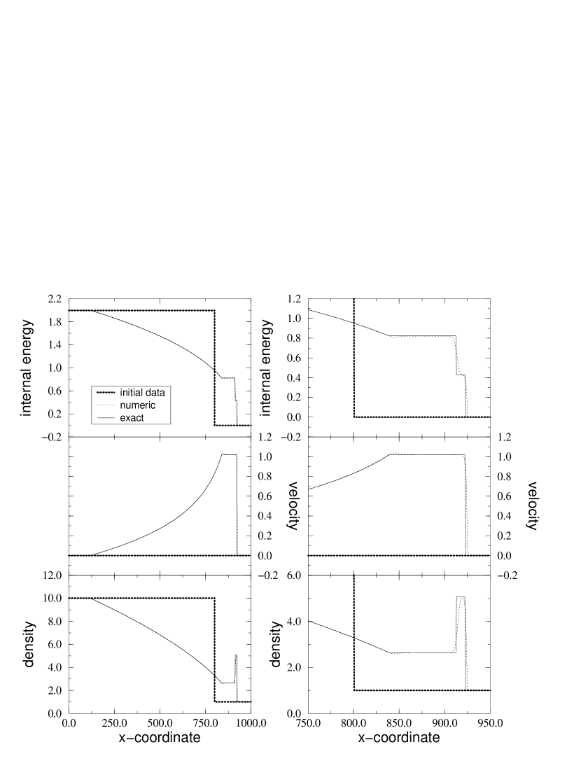
FIG. 3.: The outgoing shock tube problem (case 1). Exact versus numerical solution at an advanced time $v=270$. The domain extends from $x=0$ to $x=1000$ and a grid of 2000 zones is used ($\Delta x=0.5$). From top to bottom we plot the internal energy, velocity and density. The right panels show a zoomed view of the left panels focusing on the most interesting region. The thick dashed line shows the location of the initial discontinuity. The solid line is the exact solution and the dotted line is the numerically computed one. Those features of the solution moving to the right, i.e., the shock wave and contact discontinuity, are less developed than those moving to the left, i.e., the rarefaction wave.

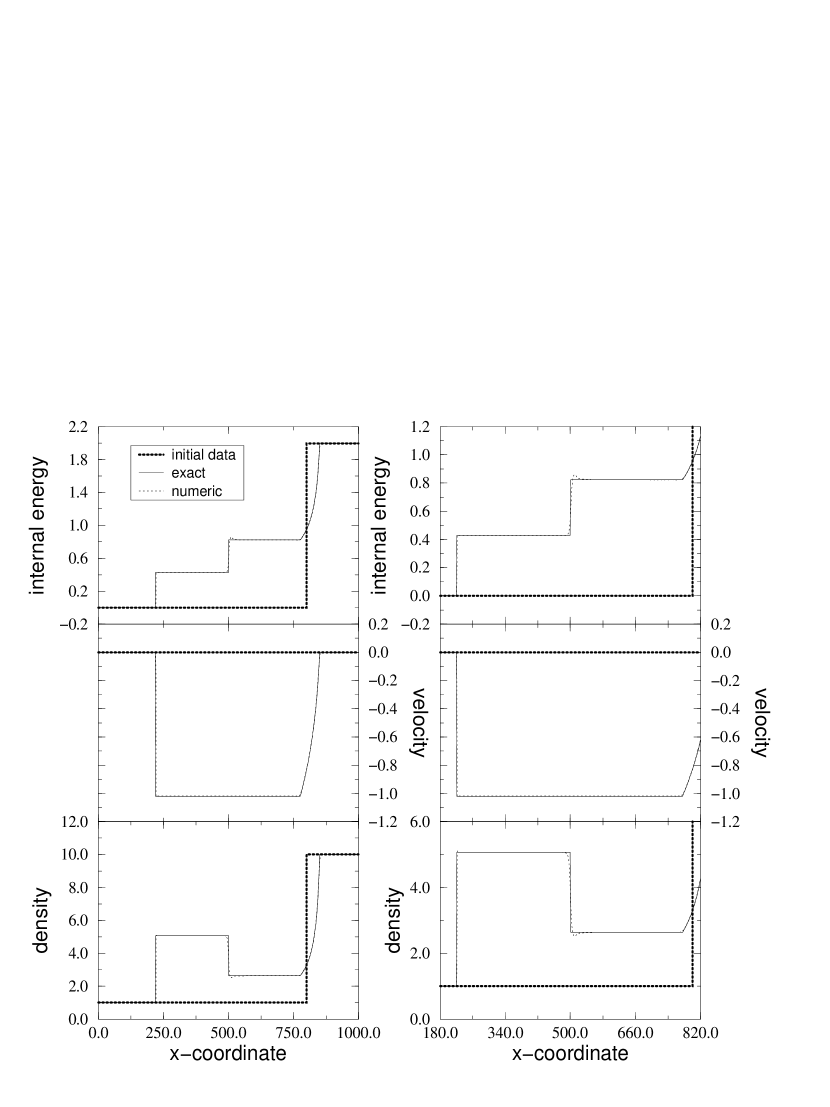
FIG. 4.: The ingoing shock tube problem (case 2). Exact versus numerical solution at an advanced time $v=120$. The domain extends from $x=0$ to $x=1000$ and a grid of 2000 zones is used ($\Delta x=0.5$). From top to bottom we plot the internal energy, velocity and density. The right panels show a zoomed view of the left panels focusing on the most interesting region. The thick dashed line shows the location of the initial discontinuity. The solid line is the exact solution and the dotted line is the numerically computed one. As in Fig. 3, those features of the solution moving to the right, i.e., the rarefaction wave, are less developed than those moving to the left, i.e., the shock wave and contact discontinuity.

FIG. 5.: Capturing the shock wave. This figure shows the different ways the shock wave is resolved in the shock tube problems 1 (ingoing; left) and 2 (outgoing; right). In spite of the fact that the grid resolution is the same in both simulations, in case 2 the shock wave is spread out in a large number of cells whereas in case 1 it is sharply captured in two zones (out of a total number of 2000 zones).

FIG. 6.: Location of the outgoing shock in the shock tube problem 1 at two different evolution times, $v=300$ and $v=600$. The numerical solution spreads the shock in a constant number of zones ($\approx 10$) from the very start and throughout the evolution.

FIG. 7.: The $L_{2}$ norm of the density function (i.e., the integrated squared difference of the numerical from the exact solution) is plotted against time, for four successive doublings of the grid size (curves A,B,C,D). The norm converges to third order. This can be seen in the insert, where the final values of the norm at $v=40$ are plotted against grid size (diamonds). The best linear fit, represented by the line, has slope 3.05. This implies that the local error is second order.

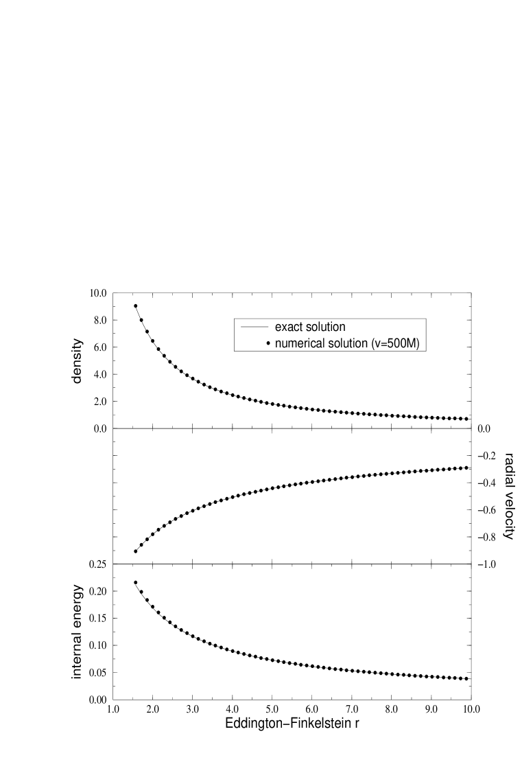
FIG. 8.: Perfect fluid spherical accretion in ingoing Eddington-Finkelstein coordinates (test fluid limit). This figure compares the exact (solid lines) and numerical (filled circles) solutions for the hydrodynamical primitive variables, as a function of the radial coordinate. The numerical solution is evolved up to a time $v=500M$. From top to bottom we plot the density, velocity and internal energy. The domain extends from $1.5M$ to $30M$ and a uniform grid of 200 zones is used. Only the first $10M$ are shown.

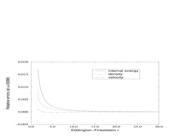
FIG. 9.: Perfect fluid spherical accretion in ingoing Eddington-Finkelstein coordinates (test fluid limit): relative errors of the primitive variables. The maximum errors are less than 2% for the internal energy, 1% for the density and 0.1% for the velocity. These numbers correspond to a simulation using 200 radial zones in the interval $1.5M-30M$ and for an evolution up to $v=500M$ into the future.

FIG. 10.: Perfect fluid spherical accretion in ingoing Eddington-Finkelstein coordinates (test fluid limit): converging towards the stationary state. The four curves, labeled A,B,C,D, present the time evolution of the density $L_{2}$ error norm (see Fig. 7 for definition), for successive doublings of the resolution. The insert shows the convergence of the norm at final time ($v=200M$). The diamonds are measured values, the line is a linear best fit with slope 2.9. Of interest in this plot is the fast approach of the numerical solution to a steady state.

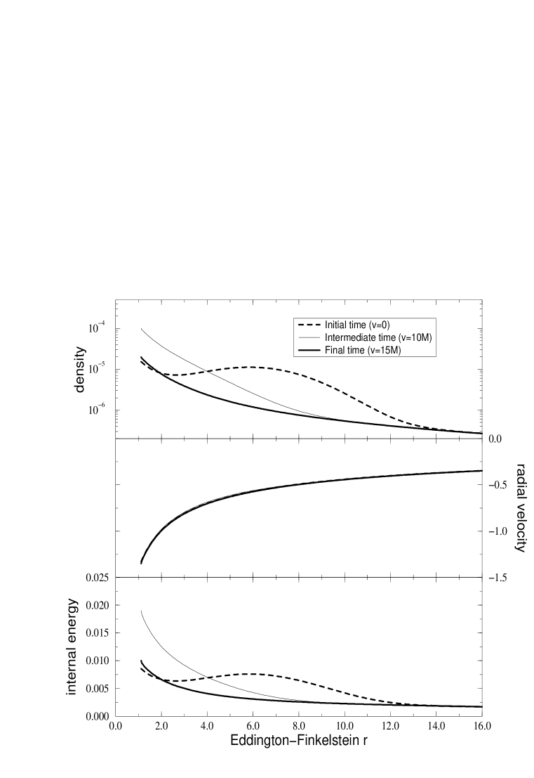
FIG. 11.: Spherical accretion of a self-gravitating perfect fluid: evolution of the primitive variables. Ingoing Eddington-Finkelstein coordinates are used, in a grid of 500 zones spanning the radial interval between $1.1M$ and $20M$. Three different times of the evolution are shown: $v=0$ (dotted thick line), $v=10M$ (solid thin line) and $v=15M$ (solid thick line). The spherical shell, centered at $r=6M$, is radially advected towards the hole. A final quasi-stationary (Bondi) solution is achieved.

FIG. 12.: Spherical accretion of a self-gravitating perfect fluid: evolution of the Riemann scalar curvature for the same simulation of Fig. 11. Notice the non-vanishing self-gravity of the initial distribution, demonstrated by a curvature profile deviating significantly from the monotonic profile of a vacuum black hole. Once the shell is accreted, the solution is once again dominated by the curvature of the final vacuum black hole spacetime.

FIG. 13.: Spherical accretion of a self-gravitating perfect fluid: evolution of the black hole apparent horizon mass. The mass of the apparent horizon shows a rapid increase in the first $15M$ (enlarged in the insert), in coincidence with the most dynamical accretion phase. The slow, quasi-steady growth at later times is the quiet response of the black hole to the low mass accretion rate imposed at the world tube. This rate can be made negligibly small (if desired).

REFERENCES

- [1]
-
[2]
http://asca.gsfc.nasa.gov/docs/xte/
-
[3]
http://www.ligo.caltech.edu
- [4] K. Thorne. In E. W. Kolb and R. Peccei, editors, Proceedings of the Snowmass 95 Summer Study on Particle and Nuclear Astrophysics and Cosmology, Singapore, 1996. World Scientific.
- [5] M. J. Rees. In R. Wald, editor, ‘Black Holes and Relativity’, Proceedings of Chandrasekhar Memorial Conference Chicago, Dec. 1996.
- [6] M. Ruffert and H.-Th. Janka, 1998, A&A, 338, 535
- [7] P. Anninos, K. Camarda, J. Masso, E. Seidel, W.-M. Suen and J.Towns, 1995, Phys. Rev. D 52, 2059-2082
- [8] C. Bona, J. Masso, E. Seidel and P. Walker, 1998, submitted to Phys. Rev. D (gr-qc/9804052)
- [9] J.A. Font, M. Miller, W.-M. Suen and M. Tobias, 1999, Phys. Rev. D, accepted (gr-qc/9811015)
- [10] G.B. Cook et al., 1998, Phys. Rev. Lett., 80, 2512-2516
- [11] K. New, K. Watt, C.W. Misner and J.M. Centrella, 1998, Phys. Rev. D 58, 064022
- [12] H. Bondi, M.J.G. van der Burg and A.W.K. Metzner, 1962, Proc. R. Soc. London, Sect. A 269 21
- [13] R.K. Sachs, 1962, Proc. R. Soc. London, Sect. A, 270 103
- [14] J. Winicour, Living Reviews in Relativity, 1998-5
- [15] R. Gómez, P. Papadopoulos and J. Winicour, 1994, J. Math. Phys., 35, 4184
- [16] Gómez, R., et al., 1998, Phys. Rev. Lett., 80, 3915
- [17] P. Papadopoulos and J.A. Font, 1999, Phys.Rev. D, 59, 044014
- [18] C.W. Misner, K.S. Thorne and J.A. Wheeler, Gravitation, W.H. Freeman and Co. (1973)
- [19] J.R. Wilson, 1972, ApJ, 173, 431
- [20] J.M. Martí, J.M. Ibáñez,, and J.A. Miralles, 1991, Phys. Rev. D, 43, 3794
- [21] F. Banyuls, J.A. Font, J.M. Ibáñez, J.M. Martí, and J.A. Miralles, 1997, ApJ, 476, 221
- [22] J.M. Ibáñez, and J.M. Martí, 1999, J. Comput. Appl. Math., in press
- [23] E. Gourgoulhon, 1991, A&A, 252, 651
- [24] S. Bonazzola, E. Gourgoulhon, and J.A. Marck, 1998, Phys. Rev. D, 58, 4020
- [25] P.J. Mann, 1991, Comput. Phys. Commun., 67, 245
- [26] E. Chow, and J.J. Monaghan, 1997, J. Comput. Phys., 134, 296
- [27] P. Laguna, 1995, Astrophys. J. 439, 814
- [28] R.A. Isaacson, J.S. Welling, and J. Winicour, 1983, J. Math. Phys., 24, 1824
- [29] N. Bishop, R. Gómez, L. Lehner, M. Maharaj, and J. Winicour, 1999, submitted to Phys. Rev. D. (gr-qc/9901056)
- [30] J. C. Miller and S. Motta, 1989, Class. Quantum Grav., 6, 185
- [31] M. Dubal, R. d’Inverno, and J.A. Vickers, 1998, Phys. Rev. D, 58, 4019
- [32] Contrast those definitions with the usual spacelike approach, in which the normal to a time-slice along with the projection operator are applied to the stress-energy tensor to obtain its Eulerian, “instantaneous rest frame”, components.
- [33] We make here the clarification that the name conservation law, used for the system of equations (6) is a well established misnomer, as the quantities are not strictly conserved in a general spacetime.
- [34] J.A. Font, J.M. Ibáñez, A. Marquina and J.M. Martí, 1994, A&A, 282, 304
- [35] J.M. Martí, and E. Müller, 1996, J. Comput. Phys., 123, 1
- [36] R.D. Richtmyer, and K.W. Morton, 1967, Difference methods for initial-value problems (Interscience, New York)
- [37] P.L. Roe, 1981, J. Comput. Phys., 43, 357
- [38] F. Eulderink, and G. Mellema, 1995, A&ASS, 110, 587
- [39] R. Donat, and A. Marquina, 1996, J. Comput. Phys., 125, 42
- [40] R. Donat, J.A. Font, J.M. Ibáñez, and A. Marquina, 1998, J. Comput. Phys., 146, 58
- [41] S.K. Godunov, Mat. Sb. 1959, 47, 271 (in Russian)
- [42] J.M. Martí, and E. Müller, 1994, J. Fluid Mech., 258, 317
- [43] L.A. Tamburino, and J. Winicour, 1966, Phys. Rev., 150, 4, 1039
- [44] We present equations and solutions corresponding to an ingoing null foliation, in keeping with the applications that follow. A trivial change in variables produces the outgoing version, which would be more appropriate e.g., for global studies of relativistic stars.
- [45] R.L. Marsa, and M.W. Choptuik, 1996, Phys. Rev. D, 54, 4929
- [46] J. Thornburg, 1987, Class. Quantum Grav., 4, 1119
- [47] E. Seidel and W.-M. Suen, 1992, Phys. Rev. Lett., 69, 1845
- [48] M.A. Scheel et al, 1995, Phys. Rev. D, 51, 4208
- [49] P. Papadopoulos, and J.A. Font, 1998, Phys. Rev. D, 58, 024005
- [50] J.A. Font, J.M. Ibáñez, and P. Papadopoulos, 1998, ApJ, 507, L67
- [51] J.A. Font, J.M. Ibáñez, and P. Papadopoulos, 1999, MNRAS, in press
- [52] H. Bondi, 1952, MNRAS, 112, 195
- [53] F.C. Michel, 1972, Ap. Space Sci. 15, 153
- [54] S. Brandt, J.A. Font, J.M. Ibáñez, J. Masso and E. Seidel, 1998, submitted to Phys. Rev. D (gr-qc/9807017)