Canonical and path integral quantisation of string cosmology models

Abstract

We discuss the quantisation of a class of string cosmology models that are characterized by scale factor duality invariance. We compute the amplitudes for the full set of classically allowed and forbidden transitions by applying the reduce phase space and the path integral methods. We show that these approaches are consistent. The path integral calculation clarifies the meaning of the instanton-like behaviour of the transition amplitudes that has been first pointed out in previous investigations.

1 Introduction

String theory, thanks to its duality symmetries, provides a cosmological scenario [1, 2, 3] in which the Universe starts from the perturbative vacuum of (super)string theory and evolves in a ‘pre-big bang’ (PRBB) phase [1, 2] characterized by an accelerated growth of the curvature and of the string coupling.

One of the main problems of string cosmology is the understanding of the mechanism responsible for the transition (‘graceful exit’) from the inflationary PRBB phase to the deflationary ‘post-big bang’ phase (POBB) with decreasing curvature that is typical of the standard cosmological scenario. Necessarily, the graceful exit involves a high-curvature, strong coupling, regime where higher derivatives [4] and string loops terms must be taken into account. In [5] it has been shown that for any choice of the (local) dilaton potential no cosmological solutions that connect smoothly the PRBB and POBB phases do exist. As a consequence, at the classical level higher order corrections cannot be ‘simulated’ by any realistic dilaton potential.

At the quantum level the dilaton potential may induce the transition from the PRBB phase to the POBB phase. In this context, using the standard Dirac method of quantisation based on the Wheeler-De Witt equation [6] a number of minisuperspace models have been investigated in the literature [7, 8, 9]. The result of these investigations is a finite, non-zero, transition probability PRBB $\rightarrow$ POBB with a typical ‘instanton-like’ dependence ($\sim\,\exp\{-1/g^{2}\}$) on the string coupling constant [7, 8].

The aim of this paper is to present a refined analysis of the quantisation of string cosmological models. To this purpose we reconsider the minisuperspace models that have been previously investigated in [7, 8, 9]. We have several motivations for doing this.

First of all, these systems are invariant under reparametrisation of time. So their quantisation requires a careful discussion of the subtleties that are typical of the quantisation of gauge invariant systems (e.g. gauge fixing) [10, 11]. Furthermore, we want to investigate the graceful exit in string cosmology using different techniques of quantisation and illustrate a consistent approach to the problem that can be successfully applied to a large class of models.

We deal with a class of string inspired models – see (2.8) and (2.9) below – that are exactly integrable and we apply the standard techniques for the canonical quantisation of constrained systems [12, 13, 14]. Using the reduced-phase space formalism we determine the positive norm Hilbert space of states. We construct the PRBB and POBB wave functions that are normalized with respect to the inner product of the Hilbert space. These wave functions are then used to compute transition amplitudes. Further, we compute the (semiclassical) transition amplitude PRBB $\rightarrow$ POBB by the path integral approach. The result agrees with the semiclassical limit of the transition amplitude that has been obtained in the reduced-phase space approach and makes clear the instanton-like structure pointed out in [7, 8]. Let us stress that our investigation is important at least for two reasons: First, the model that we are discussing is (to our knowledge) the only known example of a minisuperspace model where exact transition probabilities between two classically disconnected backgrounds have been calculated. Second, our analysis completes the previous investigations of [7, 8, 9] and allows for a systematic discussion of both classically allowed and classically forbidden transitions.

The outline of the paper is as follows. Sect. 2 is devoted to the classical theory. We derive the solutions of the equations of motion and discuss the classical behaviour of the PRBB and POBB branches. In Sect. 3 we quantise the model. This task is completed using first the canonical approach and then the path integral formalism. Eventually, we state our conclusions in Sect. 4.

2 Classical theory

We consider the string inspired model in d+1 dimensions described by the action (we assume that only the metric and the dilaton contribute non-trivially to the background)

$$S=\frac{1}{2\,\lambda_{s}^{{\rm d}-1}}\,\int\,d^{{\rm d}+1}x\,\sqrt{|g|}\,e^{-\phi}\,\left(R+\partial_{\mu}\phi\partial^{\mu}\phi-V(g_{\mu\nu},\phi)\right)\,,$$ (2.1)

where $\phi$ is the dilaton field, $\lambda_{s}=(\alpha^{\prime})^{1/2}$ is the fundamental string length parameter, and $V(g_{\mu\nu},\phi)$ is a potential term. When the latter is absent, (2.1) coincides with the tree-level, lowest order in $\alpha^{\prime}$, string effective action [15] defined in the ‘String Frame’, where the metric $g_{\mu\nu}$ coincides with the $\sigma$-model background metric that couples directly to the strings.

We deal with isotropic, spatially flat, cosmological backgrounds parametrized by

$$g_{\mu\nu}={\rm diag}\left(-N^{2}(t),a^{2}(t)\delta_{ij}\right)\,,\quad a=\exp\left[\Theta(t)/\sqrt{{\rm d}}\right]\,,\quad\phi=\phi(t)\,,$$ (2.2)

where $i,j=1,..$d. We also assume that the spatial sections have finite volume. For this class of backgrounds the action (2.1) reads

$$S=\int\,dt\,{\cal L}\,,~{}~{}~{}~{}~{}{\cal L}={\lambda_{s}\over 2}\,\left({1\over\mu}(\dot{\Theta}^{2}-\dot{\Phi}^{2})-\mu\,\rme^{-2\Phi}V(\Theta,\Phi)\right)\,.$$ (2.3)

where dots represent differentiation with respect to cosmic time $t$, $\mu(t)=N(t)\,e^{\Phi}\,$, and $\Phi$ is the ‘shifted’ dilaton field

$$\Phi=\phi-\log\,\int\,d^{\rm d}x/\lambda_{s}^{\rm d}-\sqrt{{\rm d}}\,\Theta\,.$$ (2.4)

(In (2.3) we have neglected surface terms that are inessential for our purposes.) In this paper we restrict attention to models with potential term depending on the shifted dilaton $\Phi$ only. In this case (2.3) is invariant under scale factor duality transformations [1, 16]

$$\Phi\rightarrow\Phi~{}~{}~{}{\rm or}~{}~{}~{}\phi\rightarrow\phi-2{\rm d}\,\log a\,,$$ (2.5)

$$\Theta\rightarrow-\Theta~{}~{}~{}{\rm or}~{}~{}~{}a\rightarrow\frac{1}{a}\,.$$ (2.6)

Let us introduce the conjugate momenta to $\Theta$ and $\Phi$ by the Legendre transformation

$$\Pi_{\Theta}=\frac{\lambda_{s}}{\mu}\,\dot{\Theta}\,,\qquad\Pi_{\Phi}=-\frac{\lambda_{s}}{\mu}\,\dot{\Phi}\,.$$ (2.7)

Equation (2.3) can be cast in the canonical form

$$S=\int dt\,\left[\dot{\Theta}\Pi_{\Theta}+\dot{\Phi}\Pi_{\Phi}-{\cal H}\right]\,,$$ (2.8)

where

$${\cal H}=\mu(t)H\,,~{}~{}~{}~{}H={1\over 2\lambda_{s}}\left(\Pi_{\Theta}^{2}-\Pi_{\Phi}^{2}+\lambda_{s}^{2}V(\Phi)\,e^{-2\Phi}\right)\,.$$ (2.9)

In the canonical formalism $\mu$ plays the role of a non-dynamical variable that enforces the constraint $H=0$. As we do expect for a time-reparametrisation invariant system the total Hamiltonian ${\cal H}$ is proportional to the constraint [13, 14]. The equations of motion are

$${d\Theta\over d\tau}=\frac{\Pi_{\Theta}}{\lambda_{s}}\,,~{}~{}~{}~{}~{}~{}{d\Phi\over d\tau}=-\frac{\Pi_{\Phi}}{\lambda_{s}}\,,$$ (2.10)

$${d\Pi_{\Theta}\over d\tau}=0\,,~{}~{}~{}~{}~{}~{}{d\Pi_{\Phi}\over d\tau}={\lambda_{s}\over 2}\,\left(2V-\frac{dV}{d\Phi}\right)\,e^{-2\Phi}\,,$$ (2.11)

where $\tau(t)$ is

$$\tau(t)=\int^{t}ds\,\mu(s)\,.$$ (2.12)

The gauge parameter $\tau(t)$ is related to the synchronous-gauge time $t^{(sg)}$ ($N=1$) by the relation

$$t^{(sg)}(\tau)=\int^{\tau}ds\,e^{-\Phi}\,.$$ (2.13)

We consider potentials of the form

$$V(\Phi)=\lambda\,e^{-2\Phi(q-1)}\,,$$ (2.14)

where $\lambda>0$ is a dimension-two quantity (in natural units) and $q$ is a dimensionless parameter. (This class of potentials has been first discussed in [9].) For $q\neq 0$ the explicit solution of the equations of motion (2.10), (2.11) is

$$\begin{array}[]{ll}\Theta=\displaystyle\Theta_{0}+\frac{k}{\lambda_{s}}\,(\tau-\tau_{0})\,,&e^{\Phi}=\displaystyle\left[{\sqrt{\lambda}\lambda_{s}\over|k|}\,\hbox{\rm sinh}\left({|kq|\over\lambda_{s}}|\tau-\tau_{0}|\right)\right]^{1/q}\,,\\ \\ \Pi_{\Theta}=k\,,&\displaystyle\Pi_{\Phi}=-k\,\hbox{\rm coth}\left[{kq\over\lambda_{s}}(\tau-\tau_{0})\right]\,.\end{array}$$ (2.15)

(The case $q=0$ corresponds – modulo a redefinition of $k$ – to the ‘vacuum’ solutions discussed in [1, 2, 3].) Let us determine which values of $q$ do allow for the existence of an inflationary expanding PRBB branch and a decelerating POBB branch. According to the general analysis of [1, 2], the expanding PRBB and POBB branches are defined by

$${\rm PRBB}: ~{}~{}~{}~{}{\bf H}>0\,,~{}~{}~{}~{}\dot{{\bf H}}>0\,,~{}~{}~{}~{}\dot{\Phi}>0\,,$$ (2.16)

$${\rm POBB}: ~{}~{}~{}~{}{\bf H}>0\,,~{}~{}~{}~{}\dot{{\bf H}}<0\,,~{}~{}~{}~{}\dot{\Phi}<0\,,$$ (2.17)

where

$${\bf H}=\frac{d~{}~{}}{dt^{(sg)}}\,(\log a)=\frac{1}{\sqrt{{\rm d}}}\,\frac{k}{\lambda_{s}}\,e^{\Phi}\,,$$ (2.18)

$$\dot{{\bf H}}=\frac{d~{}~{}}{dt^{(sg)}}\,{\bf H}=\frac{1}{\sqrt{{\rm d}}}\,\frac{k}{2\lambda_{s}}\,\frac{d~{}}{d\tau}\,(e^{2\Phi})\,,$$ (2.19)

$$\dot{\Phi}=\frac{d~{}~{}}{dt^{(sg)}}\,\Phi=\frac{d}{d\tau}\,(e^{\Phi})\,.$$ (2.20)

From (2.18) it is straightforward to see that expanding and contracting backgrounds are identified by $k>0$ and $k<0$ respectively. $k=0$ corresponds to the flat (d+1)-dimensional Minkowski space. Since we are interested in expanding backgrounds here and throughout the paper we shall consider only positive values of $k$, i.e. solutions with $\Pi_{\Theta}>0$. For $q\leq 1$ we have two distinct branches corresponding to PRBB and POBB states. (The limiting case $q=1$ corresponds to a positive constant potential in (2.1). The relative classical solutions have been discussed in [17].) The PRBB $(+)$ and POBB $(-)$ branches are identified by negative and positive values of $\Pi_{\Phi}$ respectively. Asymptotically, for $0<q\leq 1$ we have

$$\lim_{\Phi\rightarrow+\infty}\Pi^{(\pm)}_{\Phi}=\mp k\,,~{}~{}~{}~{}~{}\lim_{\Phi\rightarrow-\infty}\Pi^{(\pm)}_{\Phi}\sim\mp\lambda_{s}\sqrt{\lambda}e^{-q\Phi}\,,$$ (2.21)

in the strong and weak coupling regime respectively. Conversely, for $q<0$ we have

$$\lim_{\Phi\rightarrow+\infty}\Pi^{(\pm)}_{\Phi}\sim\mp\lambda_{s}\sqrt{\lambda}e^{-q\Phi}\,,~{}~{}~{}~{}~{}\lim_{\Phi\rightarrow-\infty}\Pi^{(\pm)}_{\Phi}=\mp k\,.$$ (2.22)

Substituting (2.15) in (2.13) the synchronous-gauge time $t^{(sg)}$ can be written explicitly in terms of $\tau$. We distinguish two different cases:

i) $q\neq\frac{1}{2m+1}$, $m=0,1,2,...$

$$t^{(sg)}-t^{(sg)}_{0}= -{\sigma(q)\sigma(\tau-\tau_{0})\over\sqrt{\lambda}|q-1|}\left(\frac{\sqrt{\lambda}\lambda_{s}}{k}\right)^{1-1/q}\cdot$$

$$\cdot[\,\hbox{\rm sinh}(x)]^{1-1/q}F\left({\scriptstyle\frac{\scriptstyle 1}{\scriptstyle 2},\frac{\scriptstyle q-1}{\scriptstyle 2q},\frac{\scriptstyle 3q-1}{\scriptstyle 2q}},-\hbox{\rm sinh}^{2}x\right)\,,$$

where $\sigma$ is the sign function, $F$ is the hypergeometric function [20], and

$$x=\frac{k}{\lambda_{s}}|q(\tau-\tau_{0})|\,;$$

ii) $q=\frac{1}{2m+1}$, $m=0,1,2,...$

$$t^{(sg)}-t^{(sg)}_{0}=-{\sigma(\tau-\tau_{0})\over 2\sqrt{\lambda}|q|}\left(\frac{\sqrt{\lambda}\lambda_{s}}{k}\right)^{1-1/q}\frac{\Gamma(m+1/2)}{\sqrt{\pi}\Gamma(m+1)}f(m,x)\,,$$

where

$$f(0,x)=4\,\hbox{\rm arcoth}(e^{x})\,,$$

and

$$f(m,x)=(-1)^{m}\,f(0,x)+\hbox{\rm cosh}(x)\sum_{k=0}^{m-1}\frac{(-1)^{k}\Gamma(m-k)\sqrt{\pi}}{\Gamma(m+1/2-k)[\hbox{\rm sinh}(x)]^{2(m-k)}}$$

for $m>0$. The above relations determine the PRBB and POBB branches in terms of the synchronous-gauge time $t^{(sg)}$ for different values of the parameter $q$. In particular, we have

a) $q<0$. In this case the PRBB and POBB branches are defined for

$$\begin{array}[]{rllrll}-\infty&<\tau-\tau_{0},<0&\rightarrow&-\infty&<t^{(sg)}-t^{(sg)}_{0}&<0\,,\\ 0&<\tau-\tau_{0}<\infty&\rightarrow&0&<t^{(sg)}-t^{(sg)}_{0}&<\infty\,,\end{array}$$ (2.23)

respectively.

b) $q=\frac{1}{2m+1}$. The PRBB and the POBB branches are defined for

$$\begin{array}[]{rllrll}0&<\tau-\tau_{0}<\infty&\rightarrow&-\infty&<t^{(sg)}-t^{(sg)}_{0}&<0\,,\\ -\infty&<\tau-\tau_{0}<0&\rightarrow&0&<t^{(sg)}-t^{(sg)}_{0}&<\infty\,,\end{array}$$ (2.24)

respectively. This can be checked using the asymptotic expansions of $f(m,x)$ for $x\to 0$ and $x\to+\infty$.

c) $0<q<1$, $q\neq\frac{1}{2m+1}$ . The PRBB branch is defined for

$$0<\tau-\tau_{0}<\infty~{}\rightarrow~{}\infty<t^{(sg)}-t^{(sg)}_{0}<-T\,,$$

and the POBB branch for

$$-\infty<\tau-\tau_{0}<0~{}\rightarrow~{}T<t^{(sg)}-t^{(sg)}_{0}<\infty\,,$$

where

$$T=\frac{1}{2\sqrt{\pi}|q|}\,\left(\frac{\sqrt{\lambda}\lambda_{s}}{k}\right)^{1-1/q}\,\Gamma\left(\frac{q-1}{2q}\right)\,\Gamma\left(\frac{1}{2q}\right)\,.$$

As it has been pointed out in [8, 9], in terms of the synchronous-gauge time $t^{(sg)}$ the PRBB and POBB branches are separated by a finite interval $\Delta t^{(sg)}=2T$. However, the separation between the two branches has not physical meaning. Indeed, due to the presence of a singularity in the curvature and in the string coupling the PRBB and POBB solutions are disjoint. Therefore, it is possible to define the initial value of $t$ such that the singularity occurs at $t^{sg}=0$ in both branches.

3 Quantum theory

The string cosmological model of Sect. 2 is described by a time-reparametrisation invariant Hamiltonian system with two degrees of freedom. Though its quantisation involves subtleties typical of gauge invariant systems [10, 11, 18] the standard techniques of quantisation of constrained systems can be applied straightforwardly, thanks to the integrability properties of the model [12, 13, 14].

The starting point is the canonical action (2.8). Since the constraint $H$ is of the form $H=H_{\Theta}(\Theta)+H_{\Phi}(\Phi)$ the time parameter can be defined by a single degree of freedom. In the previous section we have seen that the sign of $\Pi_{\Theta}$ determines the contracting vs. expanding behaviour of the solutions and the sign of $\Pi_{\Phi}$ identifies the PRBB vs. POBB phases. Since we are interested in the calculation of the quantum transition probability from a (expanding) PRBB phase to a (expanding) POBB phase, it is natural to use the $(\Theta,\Pi_{\Theta})$ degree of freedom to define the time of the system and fix the gauge. In this case the eigenstates of the effective Hamiltonian are identified by a continuous quantum number $k$ corresponding to the classical value of $\Pi_{\Theta}$. Wave functions that describe expanding (contracting) solutions are eigenstates of the effective Hamiltonian with $k>0$ ($k<0$).

Let us consider the canonical transformation [10] $(\Theta,\Pi_{\Theta},\Phi,\Pi_{\Phi})\to(\Sigma,\Pi_{\Sigma},\Phi,\Pi_{\Phi})$ where

$$\Sigma=\lambda_{s}{\Theta\over\Pi_{\Theta}}\,,~{}~{}~{}~{}~{}~{}\Pi_{\Sigma}={1\over 2\lambda_{s}}\Pi_{\Theta}^{2}\,.$$ (3.1)

In terms of the new canonical variables the constraint (2.9) reads

$$H(\Sigma,\Pi_{\Sigma},\Phi,\Pi_{\Phi})=\Pi_{\Sigma}-{1\over 2\lambda_{s}}\left[\Pi_{\Phi}^{2}-\lambda\lambda_{s}^{2}e^{-2q\Phi}\right]=0\,.$$ (3.2)

From (3.2) it is straightforward to see that $\Sigma$ is canonically conjugate to $H$. Thus it defines a global time parameter [11, 19]. In particular, the gauge fixing identity can be chosen as

$$F(\Sigma;t)\equiv\Sigma+t=0\,.$$ (3.3)

Equation (3.3) fixes the Lagrange multiplier as $\mu=-1$. The gauge-fixed action reads

$$S_{\rm eff}=\int_{t_{1}}^{t_{2}}dt\,\left[\dot{\Phi}\,\Pi_{\Phi}\,-\,H_{\rm eff}(\Phi,\Pi_{\Phi})\right]\,,$$ (3.4)

where the effective Hamiltonian is

$$H_{\rm eff}(\Phi,\Pi_{\Phi})={1\over 2\lambda_{s}}\left(\Pi_{\Phi}^{2}-\lambda\lambda_{s}^{2}e^{-2q\Phi}\right)\,.$$ (3.5)

The system described by the effective Hamiltonian (3.5) is free of gauge degrees of freedom and its quantisation can be performed using the standard techniques. In the next two subsections we shall discuss the reduced phase space and path integral quantisation procedures.

3.1 Reduced phase space quantisation

The reduced phase space is described by a single degree of freedom with canonical coordinates $(\Phi\in{\vrule height=6.88889pt,width=0.50003pt,depth=0.0pt\kern-0.59998pt{\rm R}},\Pi_{\Phi}\in{\vrule height=6.88889pt,width=0.50003pt,depth=0.0pt\kern-0.59998pt{\rm R}})$. Thus there are no ambiguities in the choice of the measure in the Hilbert space: $d[\mu]=d\Phi$. In the standard operator approach the quantisation of the model is obtained by identifying the canonical coordinates with operators. In the Schrödinger representation the self-adjoint operators with respect to the measure $d[\mu]$ are

$$\Phi\to\hat{\Phi}=\Phi\,,~{}~{}~{}~{}~{}\Pi_{\Phi}\to\hat{\Pi}_{\Phi}=-i{\partial~{}\over\partial\Phi}\,.$$ (3.6)

Since the effective Hamiltonian is quadratic in the momenta there are no factor ordering ambiguities. The Schrödinger equation reads

$$-i{\partial~{}\over\partial t}\,\Psi(\Phi;t)\,=\,{1\over 2\lambda_{s}}\left[{\partial^{2}~{}\over\partial\Phi^{2}}+\lambda\lambda_{s}^{2}e^{-2q\Phi}\right]\,\Psi(\Phi;t)\,,$$ (3.7)

where $t$ is defined by (3.3). Finally, the inner product in the Hilbert space is

$$\left(\Psi_{2},\Psi_{1}\right)\,=\,\int_{-\infty}^{+\infty}d\Phi\,\Psi_{2}^{*}(\Phi;t)\,\Psi_{1}(\Phi;t)\,.$$ (3.8)

The general solution of the Schrödinger equation (3.7) can be written as

$$\Psi_{q}(\Phi;t)=\int dk\,A(k)\,\psi_{k,q}(\Phi)\,e^{-ik^{2}t/2{\lambda_{s}}}\,,$$ (3.9)

where $\psi_{k,q}(\Phi)$ is the solution of the stationary Schrödinger equation $\hat{H}_{\rm eff}\psi=E\psi$ with energy $E=k^{2}/2\lambda_{s}$

$$\left[{d^{2}~{}\over d\Phi^{2}}+\lambda\lambda_{s}^{2}e^{-2q\Phi}\right]\,\psi_{k,q}(\Phi)=-k^{2}\psi_{k,q}(\Phi)\,.$$ (3.10)

For $q\not=0$ we have

$$\psi_{k,q}(z)=A_{1}(k,q)J_{i\nu}(z)+A_{2}(k,q)Y_{i\nu}(z)\,,$$ (3.11)

where $A_{1}(k,q)$ and $A_{2}(k,q)$ are arbitrary functions, and $J_{i\nu}(z)$, $Y_{i\nu}(z)$ are the Bessel functions of the first and second kind of index $i\nu=i|k/q|$ and argument

$$z=\sqrt{\lambda}\lambda_{s}\exp(-q\Phi)/|q|\,,$$ (3.12)

respectively [20].

Since the space of the solutions (3.11) is two-dimensional we have two sets of (real) orthonormal functions with respect to the inner product (3.8) [10, 21]

$$\chi^{(1)}_{\nu}(z)=C^{(1)}\left[e^{-\pi\nu/2}H^{(1)}_{i\nu}(z)+e^{\pi\nu/2}H^{(2)}_{i\nu}(z)\right]\,,$$ (3.13)

$$\chi^{(2)}_{\nu}(z)=iC^{(2)}\left[e^{-\pi\nu/2}H^{(1)}_{i\nu}(z)-e^{\pi\nu/2}H^{(2)}_{i\nu}(z)\right]\,,$$ (3.14)

where

$$C^{(1)}=\sqrt{\nu\hbox{\rm cosh}(\pi\nu/2)\over 4\hbox{\rm sinh}(\pi\nu/2)}\,,~{}~{}~{}~{}~{}~{}C^{(2)}=\sqrt{\nu\hbox{\rm sinh}(\pi\nu/2)\over 4\hbox{\rm cosh}(\pi\nu/2)}\,,$$ (3.15)

and $H^{(1)}_{i\nu}(z)$ and $H^{(2)}_{i\nu}(z)$ are the Hankel functions of the first and second kind respectively [20].

Now let us identify the stationary wave functions that correspond to expanding PRBB and POBB phases. We discuss in detail the case $0<q\leq 1$ leaving at the end of this subsection the discussion of negative values of $q$.

From (3.1) and (3.2) it follows that ${1\over 2\lambda_{s}}\Pi_{\Theta}^{2}=H_{\rm eff}$. Thus phases that are expanding (contracting) are described by eigenstates of the effective Hamiltonian with $k>0$ ($k<0$). Expanding wave functions that correspond to PRBB and POBB can be identified by investigating the asymptotic behaviours of (3.13) and (3.14) in the weak and strong coupling regimes. For $z\to\infty$, i.e. in the weak coupling regime, the wave functions (3.13), (3.14) behave as

$$\chi^{(1)}_{\nu}(z)\approx\sqrt{2\over\pi z}\,C^{(1)}\left[e^{i(z-\pi/4)}+e^{-i(z-\pi/4)}\right]\,,$$ (3.16)

$$\chi^{(2)}_{\nu}(z)\approx i\sqrt{2\over\pi z}\,C^{(2)}\left[e^{i(z-\pi/4)}-e^{-i(z-\pi/4)}\right]\,.$$ (3.17)

By applying the momentum operator $\hat{\Pi}_{\Phi}$ to the linear combinations $\chi_{\nu}^{(\pm)}=C^{(2)}\chi^{(1)}_{\nu}\mp iC^{(1)}\chi^{(2)}_{\nu}$ we find

$$\hat{\Pi}_{\Phi}\chi_{\nu}^{(\pm)}\sim\mp\lambda_{s}\sqrt{\lambda}\,e^{-q\Phi}\chi_{\nu}^{(\pm)}\,.$$ (3.18)

Thus the wave functions corresponding to PRBB and POBB in the weak coupling regime are proportional to the linear combinations $\chi_{\nu}^{(\pm)}$ respectively. The normalized PRBB and POBB wave functions in the weak coupling regime are

$$\psi^{\rm(\pm)}_{W}={1\over\sqrt{2\hbox{\rm coth}(\pi\nu)}}\left[\sqrt{\hbox{\rm tanh}(\pi\nu/2)}\chi^{(1)}_{\nu}\mp i\sqrt{\hbox{\rm coth}(\pi\nu/2)}\chi^{(2)}_{\nu}\right]\,.$$ (3.19)

By a similar argument we find that the normalized wave functions that correspond to expanding PRBB and POBB phases in the strong coupling regime are

$$\psi^{\rm(\pm)}_{S}={1\over\sqrt{2}}\left[\chi^{(1)}_{\nu}\mp i\chi^{(2)}_{\nu}\right]\,.$$ (3.20)

Using the two sets of wave functions (3.19) and (3.20) it is possible to compute the amplitudes that correspond to the different transitions. They are schematically represented in Fig. (1), where the amplitudes $A_{1}\dots A_{6}$ are given by the following expressions

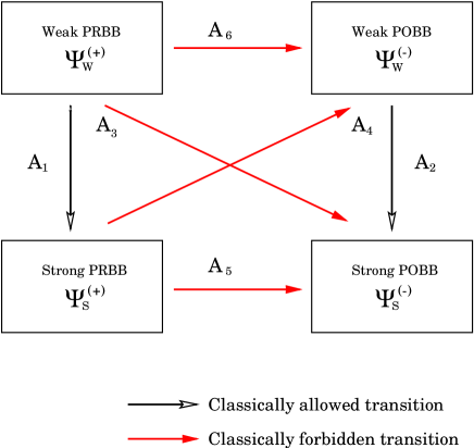
Figure 1: Different transitions in the weak and strong coupling regimes.

$$\begin{array}[]{lll}&A_{1}\equiv\left(\psi^{(+)}_{S},\psi^{(+)}_{W}\right)&=~{}{\displaystyle 1\over\displaystyle\sqrt{1+e^{-2\pi k/q}}}\,,\\ \\ &A_{2}\equiv\left(\psi^{(-)}_{S},\psi^{(-)}_{W}\right)&=~{}{\displaystyle 1\over\displaystyle\sqrt{1+e^{-2\pi k/q}}}\,,\\ \\ &A_{3}\equiv\left(\psi^{(-)}_{S},\psi^{(+)}_{W}\right)&=~{}-{\displaystyle e^{-\pi k/q}\over\displaystyle\sqrt{1+e^{-2\pi k/q}}}\,,\\ \\ &A_{4}\equiv\left(\psi^{(-)}_{W},\psi^{(+)}_{S}\right)&=~{}-{\displaystyle e^{-\pi k/q}\over\displaystyle\sqrt{1+e^{-2\pi k/q}}}\,,\\ \\ &A_{5}\equiv\left(\psi^{(-)}_{S},\psi^{(+)}_{S}\right)&=~{}0\,,\\ \\ &A_{6}\equiv\left(\psi^{(-)}_{W},\psi^{(+)}_{W}\right)&=~{}-{\displaystyle 2e^{-\pi k/q}\over\displaystyle 1+e^{-2\pi k/q}}\,.\end{array}$$ (3.21)

Let us discuss in depth the transition amplitudes (3.21). The amplitudes $A_{1}$ and $A_{2}$ correspond to classically allowed transitions. The relative transition probabilities ($P_{S,W}^{(+,+)}\equiv|A_{1}|^{2}$, $P_{S,W}^{(-,-)}\equiv|A_{2}|^{2}$) are

$$P_{S,W}^{(+,+)}=P_{S,W}^{(-,-)}={1\over 1+e^{-2\pi k/q}}\,.$$ (3.22)

For $k\to\infty$, i.e. in the semiclassical limit, (3.22) becomes

$$P_{S,W}^{(+,+)}=P_{S,W}^{(-,-)}\sim 1+O(e^{-2\pi k/q})\,,$$ (3.23)

in agreement with the classical theory. The amplitudes $A_{3}$ and $A_{4}$ describe classically forbidden transitions. The relative transition probabilities ($P_{W,S}^{(+,-)}\equiv|A_{3}|^{2}$, $P_{S,W}^{(+,-)}\equiv|A_{4}|^{2}$) are

$$P_{W,S}^{(+,-)}=P_{S,W}^{(+,-)}={e^{-2\pi k/q}\over 1+e^{-2\pi k/q}}\,.$$ (3.24)

In the semiclassical limit (3.24) becomes

$$P_{W,S}^{(+,-)}=P_{S,W}^{(+,-)}\sim e^{-2\pi k/q}+O(e^{-4\pi k/q})\,.$$ (3.25)

The transition probabilities (3.24) become highly suppressed for $k\gg 1$ where the evolution follows essentially the classical trajectory. In the limit $k\to 0$ (3.22) and (3.24) become

$$P_{S,W}^{(+,+)}=P_{S,W}^{(-,-)}\sim P_{W,S}^{(+,-)}=P_{S,W}^{(+,-)}\sim{1\over 2}+O(k)\,.$$ (3.26)

In the small-$k$ limit quantum effects are significant: the PRBB (POBB) phase in the weak coupling regime has the same probability of evolving in the PRBB or in the POBB phase in the strong coupling regime (and viceversa).

The probability of transition PRBB $\to$ POBB in the strong coupling regime ($P_{S,S}^{(+,-)}=|A_{5}|^{2}$) is identically zero. This can be understood looking at the asymptotic form of the potential for $\Phi\to\infty$ ($z\to 0$). Indeed, for large values of $\Phi$ the potential term in (3.10) goes asymptotically to zero. As a consequence, PRBB and POBB wave functions in the strong coupling regime behave asymptotically as free plane waves with opposite $\Pi_{\Phi}$ momentum. Since reflection of free plane waves is forbidden the quantum transition from PRBB to POBB in the strong coupling regime does not take place.

The last and most interesting result is the probability of transition from the PRBB phase in the weak coupling regime to the POBB phase in the weak coupling regime

$$P_{W,W}^{(+,-)}\equiv\left|A_{6}\right|^{2}=4{e^{-2\pi k/q}\over\left(1+e^{-2\pi k/q}\right)^{2}}\,.$$ (3.27)

The semiclassical limit of (3.27) is

$$P_{W,W}^{(+,-)}\sim 4e^{-2\pi k/q}+O(e^{-4\pi k/q})\,.$$ (3.28)

For $q=1$ the semiclassical result coincides, apart from a normalisation factor, with the ‘reflection-coefficient’ of [7, 8]. However, the result of [7, 8] should be considered as a ratio between two different transition probabilities rather than a transition probability by itself. Precisely, the reflection-coefficient defined in [7, 8] is

$$R\equiv{P_{S,W}^{(-,+)}\over P_{S,W}^{(+,+)}}=e^{-2\pi k/q}\,.$$ (3.29)

Note that the (classically forbidden) transition from the strong coupling PRBB phase to the weak coupling POBB phase is suppressed by a factor $e^{-2\pi k/q}$ with respect to the (classically allowed) transition from the strong coupling PRBB phase to the weak coupling PRBB phase.

Equations (3.23), (3.25) and (3.28) give also the asymptotic behaviours for small values of $q$ at given $k$. In this case quantum effects are negligible. When $0<q\ll 1$, the potential in the Schrödinger equation is nearly constant and the PRBB and POBB solutions are approximated by plane waves of opposite momentum along $\Phi$. In this case reflection of waves is highly suppressed.

A similar analysis can be performed for negative values of $q$. For $q<0$ the wave functions that correspond to expanding PRBB and POBB phases are

$$\psi^{(\pm)}_{W}={1\over\sqrt{2}}\left[\chi^{(1)}_{\nu}\pm i\chi^{(2)}_{\nu}\right]\,,$$

$$\psi^{(\pm)}_{S}={1\over\sqrt{2\hbox{\rm coth}(\pi\nu)}}\left[\sqrt{\hbox{\rm tanh}(\pi\nu/2)}\chi^{(1)}_{\nu}\pm i\sqrt{\hbox{\rm coth}(\pi\nu/2)}\chi^{(2)}_{\nu}\right]\,,\,.$$

The amplitudes for the various transitions can be read from (3.21) with the substitutions $A_{1}\leftrightarrow A_{2}$, $A_{5}\leftrightarrow A_{6}$, and $q\rightarrow-q$. Now the transition from the weak coupling PRBB phase to the strong coupling POBB phase is forbidden for negative values of $q$.

The results of this section show that the probabilities of classically forbidden transitions can be expressed, in the semiclassical limit, as power series of $e^{-2\pi k/|q|}$. Following [7, 8], from (2.18) and (2.4) we find

$$\exp(-2\pi k/|q|)=\exp\left(-\sqrt{4d}\,\pi\Omega_{s}\over|q|g^{2}_{s}\,\lambda^{d}_{s}\right)\,,$$ (3.30)

where $\Omega_{s}$ is the proper spatial volume and $g_{s}=e^{\phi_{s}/2}$ is the value of the string coupling when ${\bf H}=1/\lambda_{s}$. The ‘istanton-like’ behaviour of (3.30) shows that the probabilities of classically forbidden transitions are peaked in the strong coupling regime – as it has been already pointed out in [7, 8] – where all powers of $e^{-2\pi k/|q|}$ have to be taken into account. The occurence of this istanton-like behaviour will be clarified in the next subsection.

3.2 Path integral quantisation

The string cosmology model that we are considering can also be quantised using the functional approach. The aim of this subsection is to show how to compute, using the path integral formalism, the probability $P_{W,W}^{(+,-)}$ in the semiclassical limit. While in the case under investigation the semiclassical path integral calculation seems devoid of interest – we know already the exact transition probability (3.27) – nevertheless the semiclassical calculation is of primary importance if the system cannot be quantised exactly. We shall show that the functional approach – when performed appropriately – reproduces the exact result in the limit of large $k$. So it seems not unreasonable to assume that the semiclassical path integral calculation gives a sound approximation of the exact result also for those models that are not exactly solvable. In future, we aim to apply the formalism of this subsection to more realistic and interesting models of string cosmology.

The starting point of the functional approach is the path integral in the reduced space [14, 22]

$$I=\int_{\Phi(t_{1})}^{\Phi(t_{2})}\,{\cal D}\Phi\,{\cal D}\Pi_{\Phi}\,\exp\left(iS_{\rm eff}[\Phi,\Pi_{\Phi}]\right)\,,$$ (3.31)

where the effective action is given by (3.4) and (3.5). The transition amplitude $A_{6}$ is defined by (3.31) where the integral is evaluated on all paths that satisfy the boundary conditions

$$\Phi(-\infty)=-\infty\,,~{}~{}~{}~{}~{}~{}\Phi(\infty)=-\infty\,.$$ (3.32)

Since the effective Hamiltonian is quadratic in $\Pi_{\Phi}$ the integral in $\Pi_{\Phi}$ can be evaluated immediately. We obtain

$$I=\int_{\Phi(t_{1})}^{\Phi(t_{2})}\,{\cal D}\Phi\,\exp\left(i\int_{t_{1}}^{t_{2}}dt\,{\cal L}_{\rm eff}[\Phi,\dot{\Phi}]\right)\,,$$ (3.33)

where the effective Lagrangian is

$${\cal L}_{\rm eff}={\lambda_{s}\over 2}\left(\dot{\Phi}^{2}+\lambda e^{-2q\Phi}\right)\,.$$ (3.34)

It is advisable to use the variable $z$ defined in (3.12). Equation (3.34) becomes

$${\cal L}_{\rm eff}={1\over 2\lambda_{s}}\left({\lambda_{s}^{2}\over q^{2}}{\dot{z}^{2}\over z^{2}}+q^{2}z^{2}\right)\,.$$ (3.35)

Let us first consider the case $0<q\leq 1$. The path integral (3.33) must be evaluated on all trajectories that satisfy the boundary conditions

$$z(-\infty)=\infty\,,~{}~{}~{}~{}~{}~{}z(\infty)=\infty\,.$$ (3.36)

The effective Lagrangian (3.35) is singular in $z=0$. So there are no classical solutions describing a (smooth) transition between PRBB and POBB phases (see Sect. 2). However, it is possible to construct quasi-classical trajectories that satisfy the boundary conditions (3.36) and interpolate between PRBB and POBB phases.

Let us consider the analitical continuation of the variable $z$ to the complex plane. The effective Lagrangian is analytical in any point of the complex plane $({\rm Re}(z),{\rm Im}(z))$ save for $z=0$. Classically, the transition from the weak coupling PRBB phase to the weak coupling POBB phase would correspond to the trajectory starting at $z=+\infty$, going left along the real axis (PRBB phase, $\dot{\Phi}>0$), reaching the origin, and finally going right along the real axis to $z=+\infty$ (POBB phase, $\dot{\Phi}<0$). Clearly, since the Lagrangian is singular in $z=0$ a classical continuous and differentiable solution does not exist.

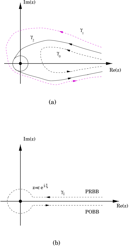
Figure 2: Contours of integration in the complex $z$-plane.

Now consider generic analytical trajectories in the complex plane that start at $Re(z)=\infty$, $Im(z)>0$, and end at $Re(z)=\infty$, $Im(z)<0$ (see Fig.2 (a)). We can divide this class of trajectories in three (topologically) distinct categories:

i) Trajectories that do not cross the imaginary axis, i.e. trajectories that cross the real axis in (at least) one point $z=z_{0}$, $Re(z_{0})>0$, $Im(z_{0})=0$ (curve $\gamma_{0}$ in Fig.2 (a));

ii) Trajectories that cross twice the imaginary axis, i.e. trajectories that cross once the real axis in $z=z_{0}$, $Re(z_{0})<0$, $Im(z_{0})=0$ (curve $\gamma_{1}$ in Fig. 2 (a));

iii) Trajectories that cross $2n$ times ($n=2,3...$) the imaginary axis, i.e. trajectories that cross $n-1$ times the positive real axis and $n$ times the negative real axis (curve $\gamma_{n}$ in Fig. 2 (a) for $n=2$);

Since the action is analytical over the entire complex plane save for $z=0$ trajectories of type $\gamma_{0}$ can be deformed continuously to a (two-folded) trajectory lying entirely on the real positive axis and defined in the interval $(Re(z_{0}),\infty)$. These curves correspond to classical solutions with the dilaton field evolving from $\Phi=-\infty$ to a maximum value $\Phi=-\ln[qRe(z_{0})/\sqrt{\lambda}\lambda_{s}]/q$ and then decreasing to $\Phi=-\infty$. A straightforward calculation shows that the action evaluated on this path is identically zero. Since (3.34) is positive definite $S_{\rm eff}=0$ can be obtained only by a time reflection, i.e. by a PRBB (POBB) phase that is covered twice. Therefore, these trajectories do not describe transitions from PRBB to POBB phases.

Let us focus attention on trajectories of type $\gamma_{1}$. They can be deformed continuously to a trajectory that lies entirely on the real positive axis except around $z=0$ where the singularity is avoided by the (small) circle $z=\varepsilon e^{i\xi}$, $\varepsilon\to 0$, $0\leq\xi<2\pi$ (see Fig.2 (b)). This trajectory describes a transition from the weak coupling PRBB phase to the weak coupling POBB phase and corresponds to a classical solution except in a small region in the strong coupling limit, where the singularity of the classical solution is avoided by the analytical continuation in the complex plane. We shall see that the path integral evaluated on this trajectory gives the leading contribution to the semiclassical approximation of the transition amplitude $A_{6}$. Trajectories of type $\gamma_{n}$ (with $n\,>\,1$) give contributes of higher order.

It is worth spending a few words on the meaning of the analytical continuation of the variable $z$ in the complex plane. Setting $z=Re^{i\xi}$ and using (2.2), (3.12) the metric is cast in the form

$$ds^{2}=-\left({qR\over\sqrt{\lambda}\lambda_{s}}\right)^{2/q}e^{2i\xi/q}\mu^{2}dt^{2}+a^{2}(t)\,dx_{i}dx^{i}\,.\\$$ (3.37)

The signature of (3.37) is a function of $\xi$. In particular, the metric (3.37) is real hyperbolic for $\xi=\pi qn$ and real Riemannian for $\xi=\pi q(2n+1)/2$, where $n$ is an integer number. Therefore, the analitic continuation of Fig.2 (b) can be interpreted as a sort of Euclidean analitical continuation in the space of metrics. Any trajectory that circles $z=0$ can be considered as an ‘$n$-instanton’ solution (with no well-defined signature) labeled by a winding number $n$ that corresponds to the number of times that the trajectory wraps around the singularity in $z=0$. In the semiclassical limit, the transition amplitude $P_{W,W}^{(+,-)}$ is given by the path integral (3.33) evaluated on the class of $n$-instanton solutions.

Let us consider the contribution to (3.33) of the one-instanton solution

$$I_{\rm sc}^{(1)}=C_{1}\exp\left(iS_{\rm eff}[z_{\gamma_{1}},\dot{z}_{\gamma_{1}}]\right)\,,$$ (3.38)

where $C_{1}$ is a normalisation factor and the subscript $\gamma_{1}$ means that the effective action is evaluated along the curve $\gamma_{1}$ of Fig.2 (b). For a trajectory with energy $k^{2}/2\lambda_{s}$ the effective action can be cast in the form

$$S_{\rm eff}=\displaystyle\int_{\gamma_{1}}\,{dz\over z}{1\over\sqrt{z^{2}+k^{2}/q^{2}}}(z^{2}+k^{2}/2q^{2})\,.$$ (3.39)

As we do expect, the effective Lagrangian has one isolated singularity in $z=0$ (pole of order one). Moreover, for $z\to\infty$ the action (3.39) shows a linear divergence. The latter is due to the asymptotic behaviour of the PRBB and POBB wave functions in the weak coupling regime. Indeed, using (3.38) and (3.39) the wave functions corresponding to the PRBB and POBB phases in the semiclassical approximation are

$$\psi^{\rm(+)} \sim\exp{\left[i\int_{\infty}^{z}\,{dz^{\prime}\over z^{\prime}}{1\over\sqrt{z^{\prime 2}+k^{2}/q^{2}}}(z^{\prime 2}+k^{2}/2q^{2})\right]}\,,$$ (3.40)

$$\psi^{\rm(-)} \sim\exp{\left[i\int_{z}^{\infty}\,{dz^{\prime}\over z^{\prime}}{1\over\sqrt{z^{\prime 2}+k^{2}/q^{2}}}(z^{\prime 2}+k^{2}/2q^{2})\right]}\,.$$ (3.41)

In the weak coupling regime ($Im(z)=0$, $z\to\infty$) (3.40) and (3.41) behave asymptotically as

$$\psi^{\rm(+)}_{z\to\infty}\sim e^{iz}\,,~{}~{}~{}~{}\psi^{\rm(-)}_{z\to\infty}\sim e^{-iz}\,,$$ (3.42)

in agreement with the asymptotic behaviour of (3.20).

The integral (3.39) can be made convergent by subtracting the asymptotic phase contribution for $z\to\infty$. Then, using the residue theorem, we obtain $S_{\rm eff}=\pi ik/q$. The amplitude (3.38) is given by

$$I_{\rm sc}^{(1)}=C_{1}e^{-\pi k/q}\,.$$ (3.43)

The semiclassical one-instanton amplitude (3.43) approximates the (exact) result for large values of $k$. This proves the consistency of the reduced phase space and path integral quantisation methods. The contribution of the $n$-instanton ($n\,>\,1$) to the transition amplitude $A_{6}$ is

$$I_{\rm sc}^{(n)}=C_{n}e^{-\pi nk/q}\,.$$ (3.44)

Hence, $n$-instanton terms give higher order contributions in the large-$k$ expansion. Equations (3.43) and (3.44) show that the instanton-like dependence (3.30) on the string coupling constant of the amplitudes that correspond to classically forbidden transitions can be traced back to the existence, in the semiclassical regime, of trajectories that connect smoothly the PRBB and POBB phases.

Let us conclude this section with two remarks. In the computation of (3.39) we have chosen only anticlockwise trajectories (see Fig. 1 (a-b)). If we considered clockwise paths the residue theorem would give $S_{\rm eff}=-\pi ik/q$ and the generic contribution to the transition amplitude would be

$$\tilde{I}_{\rm sc}^{(n)}=C_{n}e^{\pi nk/q}\,.$$ (3.45)

This result violates – in the semiclassical limit – the unitarity bound. However, there is a simple argument that allows to remove this patology. Let us consider the asymptotic behaviours of PRBB and POBB wave functions in the weak coupling regime. For complex values of $z$ (3.42) read

$$\psi^{\rm(+)}(z\to\infty)\sim e^{iRe(z)-Im(z)}\,,~{}~{}~{}~{}\psi^{\rm(-)}(z\to\infty)\sim e^{-iRe(z)+Im(z)}\,.$$ (3.46)

Since the system must be classical in the weak coupling regime the contribution to the path integral of the trajectories that approach the real axis for $z\to\infty$ must dominate the contribution of the trajectories with non-zero value of $Im(z)$. The above requirement is verified if we integrate along anticlockwise trajectories. (In this case the PRBB and POBB branches are identified by $Im(z)>0$ and $Im(z)<0$ respectively.)

For $q\,<\,0$ the transition amplitude $A_{6}$ is identically zero. Indeed, setting $w=1/z$ the effective Lagrangian (3.35) becomes

$${\cal L}_{\rm eff}={1\over 2\lambda_{s}}\left({\lambda_{s}^{2}\over q^{2}}{\dot{w}^{2}\over w^{2}}+{q^{2}\over w^{2}}\right)$$ (3.47)

and the path integral (3.33) must be evaluated on trajectories that satisfy the boundary condition $w(-\infty)=\infty$, $w(\infty)=\infty$. The action evaluated on a generic $n$-instanton solution is identically zero. Therefore, the semiclassical trajectories do not correspond to a transition between PRBB and POBB phases.

4 Conclusions

The graceful exit, i.e. the transition from the inflationary ‘pre-big bang phase’ to the deflationary ‘post-big bang’ phase is a fundamental subject of research in (quantum) string cosmology.

In this paper we have addressed this topic by investigating a special class of minisuperspace models that are invariant under scale factor duality transformations. Though this particular class of models had been previously considered in the literature [7, 8, 9] a deeper discussion was needed. Indeed, our analysis clarifies some issues of previous investigations such as the meaning of the reflection coefficient and the instanton-like behaviour of the PRBB $\to$ POBB transition, and provides new interesting results, for instance the analysis of the full set of transition amplitudes and the rôle of the semiclassical approximation.

We have shown – by a concrete example – that the reduced phase space and the path integral approaches are extremely powerful techniques of quantisation for a large class of string cosmology models. The two methods can be applied straightforwardly to any isotropic, spatially flat, model as long as the latter is characterized by scale factor duality invariance. In particular, the functional method may result very useful when the system cannot be integrated explicitly, i.e. when the Schrödinger equation (or, alternatively, the equivalent Wheeler-de Witt equation) cannot be solved exactly. Indeed, the calculation of the (semiclassical) transition amplitude between the PRBB and POBB phases in the weak coupling regime is reduced to a simple evaluation of a definite integral by means of the residue theorem. No explicit solutions of the classical equations of motion nor exact wave functions are needed.

The path integral method makes also clear a couple of other interesting features of quantum string cosmology models. First, we have proved that the instanton-like nature of the PRBB $\to$ POBB transition amplitude [7, 8] is just a consequence of the presence of the classical singularity in the strong coupling regime. Indeed, the mere existence of the singularity implies that any semiclassical trajectory gives a $n$-instanton contribution to the PRBB $\to$ POBB transition amplitude. Second, we have clarified the rôle of the functional form of the dilaton potential in the transition process. We have mentioned that the dilaton potential may ‘mimic’ – at the quantum level – high order corrections to the low-energy effective string theory action. The path integral approach shows that the calculation of the semiclassical transition amplitude PRBB $\rightarrow$ POBB does not require the knowledge of the exact functional form of the dilaton potential. The semiclassical contribution to the transition amplitude is determined uniquely by the behaviour of the dilaton potential in the strong coupling region. Thus for any dilaton potential whose asymptotic behaviour for $\Phi\to\infty$ is $V\sim e^{a\Phi}$, where $a$ is a real positive parameter, the transition amplitude (in the semiclassical approximation) is known.

Let us conclude with an interesting speculation. The transition from the PRBB phase to the POBB phase can be (phenomenologically) described by an analytical continuation of the dilaton field to complex values. We have seen in Sect. 3.2 that this analytical continuation can be interpreted in terms of a set of (complex) metrics with no well-defined signature. This way of looking at an analytical continued solution as a quantum bridge connecting two classical hyperbolic spaces has strong resemblance with the semiclassical Euclidean wormhole picture. Euclidean wormholes are classical instanton solutions of gravity-matter systems that (asymptotically) connect two manifolds [23]. They are usually interpreted as tunnelling between the two asymptotic configurations. In our case the transition from the PRBB phase to the POBB phase – at the semiclassical level – can be seen precisely as a wormhole-like effect. Our investigation provides the first example of the calculation of a wormhole-like tunnelling probability beyond the semiclassical level. This interpretation is very intriguing and supportes the interesting suggestion that singularities in the classical domain of physical, hyperbolic solutions in gravity theories can be avoided by complex solutions joining two spaces, as it happens in the case that we have discussed here.

References

References

- [1] Veneziano G 1991 Phys. Lett.B265 387
- [2] Gasperini M, Veneziano G 1993 Astropart. Physics 1 317; a complete up-date collection of papers on string cosmology can be found in http://carmen.to.infn.it/\̃hbox{}gasperin/.
- [3] Gasperini M, Veneziano G 1993 Mod. Phys. Lett. A83 701; 1994 Phys. Rev.D50 2519
- [4] See e.g. Gasperini M, Maggiore M, Veneziano G 1997 Nucl. Phys.B494 315
- [5] Brustein R, Veneziano G. 1994 Phys. Lett.B329 429; Kaloper N, Madden R, Olive KA 1995 Nucl. Phys.452 677; 1996 Phys. Lett.B371 34; Easther R, Maeda K, Wands, D 1996 Phys. Rev.D53 4247.
- [6] De Witt BS 1967 Phys. Rev.160 1113; Wheeler JA 1968 Battelle Rencontres ed C De Witt and J A Wheeler (New York: Benjamin).
- [7] Gasperini M, Veneziano G 1996 Gen. Rel. Grav. 28 1301-1307
- [8] Gasperini M, Maharana J,Veneziano G 1996 Nucl. Phys.B472 349-360
- [9] Maharana J, Mukherji S, Panda S 1997 Mod. Phys. Lett. A12 447.
- [10] Cavaglià M, de Alfaro V 1997 Gen. Rel. Grav. 29 773
- [11] Cavaglià M 1998 Approximate Canonical Quantization for Cosmological Models, to appear in: Int. J. Mod. Phys. D
- [12] Dirac P.A.M. 1964 Lectures on Quantum Mechanics, Lectures Given at Yeshiva University (New York:Belfer Graduate School of Science,Yeshiva University)
- [13] Hanson A, Regge T and Teitelboim C 1976 Constrained Hamiltonian Systems (Roma:Accademia Nazionale dei Lincei)
- [14] See e.g. Henneaux M and Teitelboim C 1992 Quantization of Gauge Systems (New Jersey: Princeton Univ. Press)
- [15] See e.g. Metsaev RR, Tseytlin AA 1987 Nucl. Phys.B293 385
- [16] Tseytlin AA 1991 Mod. Phys. Lett. A6 1721
- [17] Muller M 1990 Nucl. Phys.B337 37; Veneziano G 1991 Phys. Lett.B265 387
- [18] Cavaglià M, de Alfaro V, Filippov AT 1995 Int. J. Mod. Phys. A10 611
- [19] Hájíček P 1986 Phys. Rev.D34 1040
- [20] See e.g. Abramowitz M, Stegun IA 1968 Handbook of mathematical functions (New York:Dover Publ.) pp 358-374
- [21] See e.g. Cavaglià M, de Alfaro V, Filippov AT 1996 Int. J. Mod. Phys. D5 227
- [22] Itzykson C and Zuber JB 1980 Quantum Field Theory (Singapore:McGraw-Hill)
- [23] See e.g. Hawking SW 1990 Mod. Phys. Lett. A5 145; Mod. Phys. Lett. A5 453; Cavaglià M, de Alfaro V, de Felice F 1994 Phys. Rev.D49 6493 and references therein