Abstract

Recent improvements in astronomical observations lead to the conclusion that the Hubble constant lies between 60 and 80 Mpc km^-1 sec^-1 and the age of the universe between 11 and 14 Gigayears. Taken together with recent observations of distant type Ia supernovae and the cosmic background radiation, these limits allow a check of the consequences of predictions made a decade ago using program universe and the combinatorial hierarchy that the ratio of baryons to photons is $1/256^{4}$ and of dark to baryonic matter is 12.7. We find that the restrictions on the matter content of the universe and the cosmological constant are within, and much tighter than, the limits established by conventional means. The situation is further improved if we invoke an estimate of the normalized cosmological constant made by E.D. Jones of $\Omega_{\Lambda}\sim 0.6$. This opens a “window of opportunity” to get the predictions of the ANPA program in front of the relevant professional community before precise observations lead to a consensus. We urge ANPA members to join us in the assault on this breach in the walls of establishment thinking.

1 Introduction

When Fredrick (Parker-Rhodes) discovered the combinatorial hierarchy [1] in 1961, the excitement arose from the successful calculation of two dimensionless, empirical ratios—the fine structure constant and the ratio of electromagnetic to gravitational forces. These numbers were already known to physicists to better accuracy than his calculation provided, but (then and now) no extant conventional theory provided a way to calculate them. These same facts held true for his subsequent calculation of the electron-proton mass ratio [2], and also for many numbers the ANPA program has produced over the years. I discussed some of the reasons why established physicists continue to ignore these results in my introductory lectures presented here a couple of years ago [3]. One basic reason is that the numbers were known before the calculations were made, leaving the program open to a charge of engaging in “numerology”.

If I had been lucky, I might have been able to predict that there are only three generations of neutrinos before SLAC and LEP demonstrated this experimentally, but I doubt that this would have made much difference to the reception of our results by most physicists. The basic difficulty remains that our line of reasoning is so foreign to most physicists that any success we have along these lines will need to be (a) dramatic, (b) timely, and (c) well publicized in the relevant professional literature before the observations are made. It looks unlikely that these conditions will be met any time before ANPA 40, so far as particle physics goes.

One reason for this paper is to point out that we may now have a better chance of getting our cosmological predictions before the relevant audience in a timely fashion than we have had with particle physics. But this “window of opportunity” may easily slip by us unless more effort is put on cosmological predictions than we have exerted in the past. Here-to-fore the basic observational cosmological parameters have been so uncertain, and the competing “conventional” theories so multifarious and speculative, that our rather precise results (for those of us who believe in program universe [4]) seemed to have little prospect of getting attention, let alone confirmation. This situation has changed quite dramatically in the last year thanks to a number of different results that restrict the Hubble constant to the range 60 to 80 km sec^-1 Mpc^-1 [5, 6], limit the age of the universe to between eleven and fourteen Gigayears [5], require the universe to have much (and perhaps more) of its expansion rate determined by a repulsive cosmological constant rather than by the lack of closure mass, and give direct measurements [7] of dark matter between the galactic clusters as well as of the dark matter surrounding them.

The almost totally unexpected result that the universe is demonstrably going to keep on expanding forever was implied by the physical interpretation of program universe tabulated in [8] a decade ago. What I called $M_{vis}$ in that table was meant to imply “electromagnetically observable” rather than “detected by recording visible light”. This ambiguity persists in the table published [9] in 1994, but the prediction presented there of the number ratio of baryons to photons, first published [10] in 1991, correctly recognizes that program universe gives, as a first approximation, baryonic matter rather than the observational parameter sometimes called “visible matter”.

The distinction between baryonic and observationally visible matter is significant because a possibly substantial and currently unknown fraction of the baryonic matter may occur in the form of “brown dwarfs”. What is important here is that our theory gives what turns out to be quite a good prediction of the baryon to photon ratio and of the ratio of dark to baryonic matter. The energy density in photons is known directly from the temperature of the cosmic background radiation. Further, since our prediction only has two categories of matter in significant quantities in this epoch, we get a prediction of the total matter density independent of answering the vexed question of how much of the non-visible but baryonic matter is in the form of brown dwarfs or other ordinary matter. Thus, knowing the Hubble constant $H_{0}$, we can predict $\Omega_{M}\equiv\rho_{m}/\rho_{c}$ where $\rho_{c}=3H_{0}^{2}/8\pi G_{N}$, $G_{N}$ being the Newtonian gravitational constant.. The absolute mass of the universe we also predicted a decade ago is still not easily connected to observational data, but even in 1989 pointed in the direction of an open universe [8], in opposition to a near consensus among the cosmological theorists.

As we will show in Section 3, taking seriously our predicted ratio of baryons to photons and of dark to baryonic matter is already quite restrictive, and well within the limits allowed by current cosmological observations. When augmented by an “a priori” estimate of the cosmological constant made by Ed Jones (cf. Section 4), we end up being able to make a prediction of the two parameters ($\Omega_{M}$ and $\Omega_{\Lambda}$) which specify the gross cosmology of the universe that is better than current observations can test. The three numbers $M_{Dark}/M_{B}$, $N_{B}/N_{\gamma}$ and $M_{\rm Univ}$ play a role in observational cosmology comparable to the role played by the three Parker-Rhodes numbers ($e^{2}/\hbar c,m_{\rm Planck}/m_{\rm proton},m_{p}/m_{e}$) in particle physics. In both observational cosmology and elementary particle physics the conventional approach requires the numbers to be taken from observation and fitted into an hypothesized theory rather than calculated from first principles. In contrast to the empirically well known Parker-Rhodes numbers, however, the first two cosmological numbers are only this year beginning to take on consensus values at the ten to twenty per cent level, and $M_{\rm Univ}$ is still know only within a factor of two or so. This time the ANPA program has a fighting chance to get our numbers in front of the relevant audience before they are well measured rather than after the fact.

How the “repulsive cosmological constant” comes about is another story, which will only be briefly touched on in this paper. Ed Jones had reached that result on quite general grounds some time ago, but unfortunately did not publish his conclusion because of lack of observational evidence. He is now preparing a short paper on the subject [11], which I pray will get into the literature in time to get him some credit.

But none of my remarks here will make sense unless we have in front of us the recent observational results which have so dramatically changed the cosmological picture.

2 A Brief Survey of Recent Cosmological Results

A number of factors, which are the culmination of many years of hard work by many astronomers, astrophysicists, and physical cosmologists, have converged rather suddenly on definite observational cosmological results. Partly these are simply the result of the accumulation of data from the large Keck telescopes in Hawaii and Chile, as well as from smaller observatories, and from the Hubble Space Telescope. Partly they are the result of accumulating satellite data, particularly from Hipparcos and the COsmic Background Experiment (COBE). But the data analysis would not have been possible without the increasing power and availability of low cost computers, and would not have yielded such dramatic results so quickly without some very clever ideas exploiting the technological and observational opportunities.

Before plunging into my description of some of the results, I wish to stress that I am an outsider in this field, and have had to rely almost exclusively on one conference this spring (DM98) and one summer institute (SSI XXVI) which I had the good fortune to attend. There was enough discussion of controversial matters in both of these environs to allow me to believe I could assess reasonably accurately the outlines of agreement that are emerging, and to draw my own conclusions. But be warned that my lack of background could have led me pretty far astray.

One basic fact which seems pretty firm is that Hipparcos has now supplied a large enough sample of cephid variables with measured parallax to change the calibration of the distance-luminosity relation by ten percent or more. So far as the age of the universe goes, it is equally important that the parallax of several globular clusters has also been measured. This turned out to make the oldest objects in our own galaxy younger than estimates of the “age of the universe” by the right amount to achieve consistency [12, 5]. Thus there is no longer an “age problem”. The universe, and its contents, have existed something like 12.5 billion ($1.25\times 10^{10}$) years, give or take a billion or so; as our reference time we take the backward extrapolation to the time when the contents of the universe must have been so compacted that the question of whether we can trust the laws of physics enough to extrapolate any earlier becomes, for some of us, the critical question. Fortunately both “fireball time” (when the radiation breaks away from the matter) and the earlier time of nucleosynthesis (when the neutrons freeze out and for a few minutes can be used to form deuterons, ${}^{3}He$, alpha particles and ${}^{7}Li$) are sufficiently later than this “epistemological cutoff” so that we can still perform relevant laboratory experiments to check our assumptions. We can remain comfortable with the cosmological calculations needed in what follows from an operational point of view.

This extrapolation back in time starts from “local” evaluations of the “Hubble Constant”—the distance-velocity relation between recessional velocity as measured by red-shift using data out to about 100 Mega-parsec ($1\ Mpc=3.26...\times 10^{6}$ light years). For the nearer galaxies this again depends on the recalibration of the cephids, but also on getting a handle on the local imhomogenieties (Virgo cluster, the “great attractor”, etc., etc.). Recently much more data has become available on the “Peculiar Velocities” of Galaxies which deviate from the average Hubble streaming. Consequently one can plot the overall distribution of gravitating matter (rather than the distribution of light) over this enormous—but still “local”—region. These measures have to be self-consistent. When this is achieved, as is claimed, it reinforces the conclusion, which now comes from several different types of data, that most of the gravitating matter in the universe is dark rather than luminous.

To take the Hubble relation back farther, one needs a “standard candle” that is reliable to as early times as is possible. It turns out that the type Ia supernovae are numerous enough in the region where cephid measurements can still be made to collect enough calibrated light curves to establish what is needed. This took a very clever combination of physical reasoning and optimal utilization of resources which have to be shared with many other meritorious observational programs. It is this data which gives firm evidence for a repulsive cosmological constant [13].

Direct measurement of the dark matter itself has been made by detailed analysis of the defects in the gravitational lenses provided by clumps of “local” galaxies imaging very early galaxies (back to red-shift 5!) [7]. Most of the lensing comes from the dark matter itself, not from the sprinkling of visible matter which, presumably, has fallen into it. Such lenses also exist between visible clumps; these lenses may or may not include burned out galaxies, but are not optically visible. These results confirm the hypothesis that much more of the gravitating matter in the universe is dark than luminous. Even with this additional matter, there is not enough to close the universe in the absence of an attractive cosmological constant, let alone enough in the presence of the observed repulsive cosmological constant. This becomes clear when the COBE data and the type Ia supernovae data are combined [14, 15].

3 Consequences of Two Program Universe Predictions

3.1 Program Universe

Here we remind the reader of how we use discrimination (“$\oplus$”) between ordered strings of zeros and ones (bit-strings) defined by

$$({\bf a}(W)\oplus{\bf b}(W))_{w}=(a_{w}-b_{w})^{2};\ \ a_{w},b_{w}\in 0,1;\ \ w\in 1,2,....,W$$ (1)

to generate a growing universe of bit-strings which at each step contains $P(S)$ strings of length $S$. We use an algorithm known as program universe which was developed in collaboration with M.J.Manthey [16, 4]. Since no one knows how to construct a “perfect” random number generator, we cannot in practice start from Manthey’s “flipbit” (which returns a zero or a one with equal probability when asked), and must content ourselves with a pseudo-random number generator that, to some approximation which we will be wise to reconsider from time to time, will come close to that performance. Using any available approximation to “flipbit” and assigning an order parameter $i\in 1,2,...,P(S)$ to each string in our array, Manthey [16] has given the coding for constructing a routine “PICK” which picks out some arbitrary string ${\bf P}_{i}(S)$ with probability $1/P(S)$. Then program universe amounts to the following simple algorithm:

PICK any two strings ${\bf P}_{i}(S)$,${\bf P}_{j}(S)$, $i,j\in 1,2,...,P$ and compare ${\bf P}_{ij}={\bf P_{i}\oplus P_{j}}$ with ${\bf 0}(S)$.

If ${\bf P}_{ij}\neq{\bf 0}$, adjoin ${\bf P}_{P+1}:={\bf P}_{ij}$ to the universe, set $P:=P+1$ and recurse to PICK. [This process is referred to as ADJOIN.]

Else, for each $i\in 1,2,...,P$ pick an arbitrary bit ${\bf a}_{i}\in 0,1$, replace ${\bf P}_{i}(S+1):={\bf P}_{i}(S)\|{\bf a}_{i}$, set $S:=S+1$ and recurse to PICK. [This process is referred to as TICK.]

Here the operation “$\|$” simply extends the string on the left of the symbol by adjoining the string to its right (in the instance above, the arbitrary bit ${\bf a}_{i}$ supplied by “flipbit”) and adjusting the ordering indices and resulting string length parameter appropriately. We note that any universe so generated is “uncrunchable”, to quote John Wheeler [17]. In our current context this construction, taken seriously, necessarily requires that the cosmological constant be greater than zero, as we will assume below.

3.2 Events, Labels, Contents

This version of program universe—called “Program Universe 2” in the published Ref. [8]—provides considerable structure to “events”, modeled by the two alternatives presented above. Note that so long as the string produced by the event is non-null (and hence that all three strings are non-null and different from each other), the string length does not change (i.e. there is no TICK). Interpreted as a three-leg Feynman diagram (a story we cannot develop to any great extent in this paper), ADJOIN can be shown to correspond to a “vacuum fluctuation” which conserves (relativistic) 3-momentum but not energy, and hence is unobservable as a physical process. On the other hand, when two indistinguishable strings are compared, producing a TICK, this can be interpreted as four-leg Feynman diagram in which one of the two indistinguishable strings was produced earlier and the other serves as the needed spectator in any observable relativistic finite particle number three body scattering process [18].

Program Universe 2 also provides a separation into a conserved set of “labels”, and a growing set of “contents” which can be thought of as the space-time “addresses” to which these labels refer. To see this, think of all the left-hand, finite length $S$ portions of the strings which exist when the program TICKs and the string-length goes from $S$ to $S+1$. Call these labels of length $L=S$, and the number of them at the critical tick $N_{0}(L)$. Further PICKs and TICKs can only add to this set of labels those which can be produced from it by pairwise discrimination, with no impact from the (growing in length and number) set of content labels with length $S_{C}=S-L>0$. If $N_{I}\leq N_{0}(S_{L})$ of these labels are discriminately independent, then the maximum number of distinct labels they can generate, no matter how long program universe runs, will be $2^{N_{I}}-1$, because this is the maximum number of ways we can choose combinations of $N_{I}$ distinct things taking them $1,2,...,N_{I}$ times. We will interpret this fixed number of possibilities as a representation of the quantum numbers of systems of “elementary particles” allowed in our bit-string universe and use the growing content-strings to represent their (finite and discrete) locations in an expanding space-time description of the universe.

This label-content schema then allows us to interpret the events which lead to TICK as four-leg Feynman diagrams representing a stationary state scattering process. Note that for us to find out that the two strings found by PICK are the same, we must either pick the same string twice or at some previous step have produced (by discrimination) and adjoined the string which is now the same as the second one picked. Although it is not discussed in bit-string language, a little thought about the solution of a relativistic three body scattering problem Ed Jones and I have found [18] shows that the driving term ($>-<\atop-$) is always a four-leg Feynman diagram ($>-<$) plus a spectator ($\ -\$) whose quantum numbers are identical with the quantum numbers of the particle in the intermediate state connecting the two vertices. The step we do not take here is to show that the labels do indeed represent quantum number conservation and the contents a finite and discrete version of relativistic energy-momentum conservation. But we hope that enough has been said to show how we could interpret program universe as representing a sequence of contemporaneous scattering processes, and an algorithm which tells us how the space in which they occur expands..

3.3 Cosmological Interpretation of Program Universe

At this point we need a guiding principle to show us how we can “chunk” the growing information content provided by discriminate closure in such a way as to generate a hierarchical representation of the quantum numbers that the label-content schema provides. Following a suggestion of David McGoveran’s [19], we note that we can guarantee that the representation has a coordinate basis and supports linear operators by mapping it to square matrices.

The mapping scheme originally used by Amson, Bastin, Kilmister and Parker-Rhodes [20] satisfies this requirement. This scheme requires us to introduce the multiplication operation ($0\cdot 0=0=0\cdot 1=0=1\cdot 0$, $1\cdot 1=1$), converting our bit-string formalism into the field $Z_{2}$. First note, as mentioned above, that any set of $n$ discriminately independent (d.i.) strings will generate exactly $2^{n}-1$ discriminately closed subsets (dcss). Start with two d.i. strings ${\bf a}$, ${\bf b}$. These generate three d.i. subsets, namely $\{{\bf a}\}$, $\{{\bf b}\}$, $\{{\bf a},{\bf b},{\bf a}\oplus{\bf b}\}$. Require each dcss ({    }) to contain only the eigenvector(s), of three $2\times 2$ mapping matrices which (1) are non-singular (do not map onto zero) and (2) are d.i. Rearrange these as strings. They will then generate seven dcss. Map these by seven d.i. $4\times 4$ matrices, which meet the same criteria (1) and (2) just given. Rearrange these as seven d.i. strings of length 16. These generates $127=2^{7}-1$ dcss. These can be mapped by 127 $16\times 16$ d.i. mapping matrices, which, rearranged as strings of length 256, generate $2^{127}-1\approx 1.7\times 10^{38}$ dcss. But these cannot be mapped by $256\times 256$ d.i. matrices because there are at most $256^{2}$ such matrices and $256^{2}\ll 2^{127}-1$. Thus this combinatorial hierarchy terminates at the fourth level. The mapping matrices are not unique, but exist, as has been proved by direct construction and an abstract proof [21]. It is easy to see that the four level hierarchy constructed by these rules is unique because starting with d.i. strings of length 3 or 4 generates only two levels and the dcss generated by d.i. strings of length 5 or greater cannot be mapped.

Making physical sense out of these numbers is a long story [3], and making the case that they give us the quantum numbers of the standard model of quarks and leptons with exactly 3 generations has only been sketched [9]. However we do not require the completely worked out scheme to make interesting cosmological predictions. The ratio of dark to “visible” (i.e. electromagnetically interacting) matter is the easiest to see. The electromagnetic interaction first comes in when we have constructed the first three levels giving 3+7+127 =137 dcss, one of which is identified with electromagnetic interactions because it occurs with probability $1/137\approx e^{2}/\hbar c$. But the construction must first complete the first two levels giving 3+7=10 dcss. Since the construction is “random” and this will happen many, many times as program universe grinds along, we will get the 10 non-electromagnetically interacting labels 127/10 times as often as we get the electromagnetically interacting labels. Our prediction of $M_{Dark}/M_{B}=12.7$ is that naive. We discuss how we might improve the calculation of this number in the concluding section.

The $1/256^{4}$ prediction for $N_{B}/N_{\gamma}$ is comparably naive. Our partially worked out scheme of relating bit-string events to particle physics [9, 3], makes it clear that photons, both as labels (which communicate with particle-antiparticle pairs) and as content strings will contain equal numbers of zeros and ones in appropriately specified portions of the strings. Consequently they can be readily identified as the most probable entities in any assemblage of strings generated by flipbit. This scheme also makes the simplest representation of fermions and anti-fermions contain one more “1” or one more “0” than the photons. (Which we call “fermions” and which “anti-fermions” is, to begin with, an arbitrary choice of nomenclature.) Since our dynamics insures conventional quantum number conservation by construction, the problem — as in conventional theories—is to show how program universe introduces a bias between “0” ’s and “1” ’s once the full interaction scheme is developed. (The recently commissioned “B-Factory at SLAC is aimed at providing experimental evidence relevant to a conventional explanation of the observed bias between matter and anti-matter in our universe.)

Since program universe has to start out with two strings, and both of these cannot be null if the evolution is lead anywhere, the first significant PICK and discrimination will necessarily lead to a universe with three strings, two of which are “1” and one of which is “0”. Subsequent PICKs and TICKs are sufficiently “random” to insure that (at least statistically) there will be an equal number of zeros and ones, apart from the initial bias giving an extra one. Once the label length of 256 is reached, and sufficient space-time structure (“content strings”) generated and interacted to achieve thermal equilibrium, this label bias for a 1 compared to equal numbers of zeros and ones will persist for 1 in 256 labels. But to count the equilibrium processes relevant to computing the ratio of baryons to photons, we must compare the labels leading to baryon-photon scattering compared to those leading to photon-photon scattering. This requires the baryon bias of 1 to appear in one and only one of the four labels of length 256 involved in that comparison; this comparison is illustrated in Fig. 1, which assumes that the above mentioned interpretation of the strings causing observable TICK’s as four leg Feynman diagrams has been satisfactorily demonstrated. We conclude that, in the absence of further information, $1/256^{4}$ is the program universe prediction for the baryon-photon ratio at the time of big bang nucleosynthesis. We will discuss how this estimate could be strengthened and refined in the concluding section.

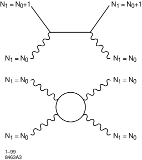
Figure 1: Comparison of bit-string labeled processes after the label length is fixed at 256 interpreted as baryon ($N_{1}=N_{0}+1$) photon ($N_{1}=N_{0}$) and photon-photon scattering. Here $N_{1}$ and $N_{0}$ symbolize, respectively, the number of ones and zeros in the label part of the string (which is of length 256). Program universe guarantees that, in the absence of further considerations, the content part of the strings will have an equal number of zeros and ones with very high probability as the string length (universe) grows.

3.4 Comparison with Observation

The currently accepted way to set the stage for the discussions of cosmology is to note that if the universe is homogeneous and isotropic on a large enough scale (for which hypothesis there is now claimed to be good evidence) and postulate Einstein gravitation (at least in the weak field limit, for which there is again good evidence) the Friedman-Robertson-Walker (FRW) equations apply. Further, if we know the boundary conditions at the time of big-bang nucleosynthesis (when the event horizon was “only” a million or so times smaller than it is now), we can integrate these equations up to the current time knowing only the two parameters $\Omega_{M}$ and $\Omega_{\Lambda}$ [22]. Here $\Omega_{M}=\rho_{M}/\rho_{c}$ is the ratio of the contemporary density of matter to the critical density in the absence of a cosmological constant ($\Omega_{\Lambda}=0$). We can get this knowing only Newton’s gravitational constant $G_{N}$ and the current value of the Hubble constant $H_{0}\equiv 100\ h_{0}\ km\ s^{-}1Mpc^{-}1$ since $\rho_{c}=3H_{0}^{2}/8\pi G_{N}=1.88\times 10^{-29}h_{0}^{2}\ g\ cm^{-3}$. Similarly the scaled cosmological constant is given by $\Omega_{\Lambda}=\Lambda c^{2}/3H_{0}^{2}$, where $\Lambda$ is the integration constant which must appear in solving the FRW differential equations.

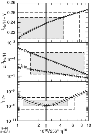
Figure 2: Comparison of the bit-string physics prediction that $\eta=256^{-4}$ with accepted limits on the cosmic abundances as given by Olive and Schramm in [23], p. 119.

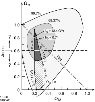
Figure 3: Limits on $(\Omega_{M},\Omega_{\Lambda})$ set by combining the Supernovae Type Ia data from Perlmutter, et al. with the Cosmic Ray Background Experiment (COBE) satellite data as quoted by Glanz [14] (dotted curves at the 68.37% and 99.7% confidence levels) with the predictions of bit-string physics that $\eta_{10}=10^{10}/256^{4}$ (cf. Fig. 1) and $\Omega_{\rm Dark}/\Omega_{B}=12.7$. We accept the constraints on the scaled Hubble constant $h_{0}=0.7\pm 0.1$ [5] and on the age of the universe $t_{0}=12.5\pm 1.5\ Gyr$ (solid lines). We include the predicted constraint $\Omega_{\Lambda}>0)$. The Jones estimate of $\Omega_{\Lambda}=0.6$ is indicated, but the uncertainty is not available.

The two program universe results we consider here are that the ratio of dark to baryonic matter is 12.7 to 1 and that the ratio of baryons to photons at the time of nucleosynthesis, symbolized by $10^{-10}\eta_{10}$, is $1/256^{4}$. Our naive arguments for these numbers are given in the last section; from now on we accept them as predictions to be tested. We show in Fig. 2 that this value for $\eta_{10}$ well represents a central value consistent with the cosmic abundances of the light elements. Since we know from the currently observed photon density (calculated from the observed $2.782\ ^{o}K$ cosmic background radiation) that the normalized baryon density is given by [22]

$$\Omega_{B}=3.67\times 10^{-3}\eta_{10}h_{0}^{-2}$$ (2)

and hence from our assumption about dark matter that the total mass mass density will be 13.7 times as large, we have that

$$\Omega_{M}=0.11706h_{0}^{-2}\ .$$ (3)

Hence, for $0.8\geq h_{0}\geq 0.6$ [6], $\Omega_{M}$ runs from $0.18291$ to $0.32517$. This clearly puts no restriction on $\Omega_{\Lambda}$.

Our second constraint comes from integrating the scaled Friedman-Robertson-Walker (FRW) equations from a time after the expansion becomes matter dominated with no pressure to the present. Here we assume that this initial time is close enough to zero on the time scale of the integration so that the lower limit of integration can be approximated by zero [24]. Then the age of the universe as a function of the current values of $\Omega_{M}$ and $\Omega_{\Lambda}$ is given by

$$t_{0} = 9.77813h_{0}^{-1}f(\Omega_{M},\Omega_{\Lambda})\ Gyr$$ (4)

$$= 9.77813h_{0}^{-1}f(0.11706h_{0}^{-2},\Omega_{\Lambda})\ Gyr$$

where

$$f(\Omega_{M},\Omega_{\Lambda})=\int_{0}^{1}dx\sqrt{{x\over\Omega_{M}+(1-\Omega_{M}-\Omega_{\Lambda})x+\Omega_{\Lambda}x^{3}}}\ .$$ (5)

For the two limiting values of $h_{0}$, we see that

$$h_{0} = 0.8,\ \ t_{0}=12.223f(0.18291,\Omega_{\Lambda})\ \ Gyr$$

$$h_{0} = 0.6,\ \ t_{0}=16.297f(0.32517,\Omega_{\Lambda})\ \ Gyr\ .$$ (6)

The results are plotted in Fig. 3.

To orient ourselves in the $(\Omega_{M},\Omega_{\Lambda})$ plane, we first consider a flat universe in which the curvature term in the normalized FRW equations vanishes, i.e. $1-\Omega_{M}-\Omega_{\Lambda}=0$. Then for $h_{0}=0.8$, performing the integration, these constraints predict $t_{0}=13.8\ Gyr$, barely within the allowed range. The upper limit of $14\ Gyr$ requires that $h_{0}=.737,\Omega_{M}=.199,\Omega_{\Lambda}=.801$. We conclude that requiring flatness together with $\eta_{10}=2.33$ and $M_{\rm Dark}/M_{B}=12.7$ restricts us to the short line segment from $(\Omega_{M},\Omega_{\Lambda})=(0.183,0.817)$ to $(0.199,0.801)$. At the same time, this sets a lower bound of $0.737$ on $h_{0}$, and of $13.8\ Gyr$ on $t_{0}$. It is therefore very important for our bit-string cosmology to know how flat it has to be. Otherwise we may soon be forced to modify or abandon this approach to cosmology as the observational data improve.

If we relax the flatness assumption, but take from our model (see Section 3.1) the requirement that the cosmological constant be repulsive (space generates more space as time goes by), the predicted limits on our parameters as plotted in Fig. 3 are well within the 99.7% confidence limit given by putting together the type Ia supernovae and the COBE data [14, 15]. At the 68.37% confidence limit provided by this data we see that, if we can find a way to justify our choice for $\eta_{10}$ and the ratio of dark to baryonic matter, we require the cosmological constant to lie between 0.45 and 0.94. We conclude that the bit-string cosmology is within the observational bounds, and that either a calculation of the limits on flatness or of the limits on the cosmological constant would greatly improve the predictive power of our theory.

4 Jones’ Cosmological Constant

Since Jones’ paper [11] is still not submitted, I am at liberty here only to quote the following sentence

From general operational arguments, Ed Jones has shown how to start from $\sim N$ Plancktons and self-generate a universe with $\sim N^{\prime}$ baryons which—for appropriate choice of $N$—resembles our currently observed universe. In particular it must necessarily have a positive cosmological constant characterized by $\Omega_{\Lambda}\sim 0.6$

We note further that Jones’ general arguments a) are completely compatible with program universe and b) do not in themselves fix the value of $N$. Further, the estimate given above, which was made before and independent of the calculations reported in the last section, falls squarely in the middle of the allowed region (see Fig. 3). Clearly, pursuing the combination of these two lines of reasoning could prove to be very exciting. We indicate how this might be done in the concluding section.

5 A Research Proposal for ANPA

We believe that the above calculations amply justify our contention made in the introduction that if the ANPA program can be shown in a convincing way to lead to the prediction of the two parameters $\eta_{10}$ and $\Omega_{\rm Dark}/\Omega_{B}$ to anything like the precision that $\hbar c/e^{2}$ and $[M_{\rm Planck}/m_{\rm proton}]^{2}$ are given in the lowest approximation by the older triumph [20] then we can provide a target for the observational cosmologists to shoot at. If that happens, as observations improve, we will be either vindicated or shown to have made some fatal flaw in our reasoning. This is a much more exciting game to play than trying to show physicists that we can approximately compute numbers that they already are confident they can measure to higher precision than we can provide.

The problem is that the naive arguments given above for the numbers studied here are—even within ANPA—unlikely to be convincing to any one other than a sympathetic reader. A friendly critic would at best characterize them as “heuristic” and a less friendly critic as “hand-waving”. A hostile critic will dismiss them as “wishful thinking.” I readily admit that we need to do better, but fear that the amount of work needed is beyond my reach. Fortunately, most of it is precisely what needs to be done in any case, if the elementary particle end of the ANPA program is not to stagnate. I now outline a possible research strategy.

I propose that we first construct a rigorous bit-string theory for renormalized QED in the truncated version of a single particle-antiparticle mass and the first combinatorial hierarchy approximation for the fine structure constant, i.e. 1/137. Basically, I believe this only involves putting together two pieces of the puzzle which have already been completed, and which we now discuss.

Following a suggestion of Feynman’s [25], Lou Kauffman and I have shown [26] that, given as the boundary condition a rational fraction velocity between two fixed end-points in 1+1 dimensional space-time, a finite and discrete version of the free particle Dirac Equation can be solved by an appropriate collection of bit-strings pairs interpreted as “random walks”. Hence, once we have shown how to couple the beginning- and end-points to bit strings representing photons which satisfy the appropriate conservation laws in three dimensions, the “renormalized single particle propagator” problem for fermions will have been solved [27].

Again following an idea originally due to Feynman [28], as presented by Dyson [29] and developed further by Tanimura [30], Kauffman and I have shown [31] that the discrete physics hypothesis that first measuring position and then velocity is different from first measuring velocity and then position leads to the relativistic commutation relations needed to undergird, rigorously, the Feynman-Dyson-Tanimura “proof” of the free particle Maxwell Equations using in addition only Newton’s second law connecting force to field. This amounts to (for a single particle trajectory) emission or absorption of “photons” at finite and discrete points in 3-space connected by straight line segments. We have noted above that these in turn can be represented by collections of random walks of a Dirac particle. What remains is to show that the “interaction” so described does indeed consistently describe the connection between bit-string photons and bit-string Dirac particles in the $\hbar c/e^{2}=137$ third level hierarchy calculation. That this way of looking at the hydrogen atom also provides the relativistic connection between binding energy, principle quantum number and coupling constant first given by Bohr [32] has already been proved [10]. Bits and pieces of the geometrical interpretation of the angles between bit-strings needed to lace all this together also exist [3].

I feel that a concerted effort could get to a lowest order renormalized QED in this way, providing the bit-string underpinning for the renormalized Feynman diagrams needed to discuss the equilibrium between protons and black body gamma radiation (Compton scattering and photon-photon scattering) to a part in 137 at the time of “big-bag nucleosynthesis”. The black-body spectrum itself is guaranteed by the statistical character of string creation in program universe and the indistinguishability (in the usual sense of Bose-Einstein statistics) of the photon states in a bit-string representation of photons. If the bit-string version of the finite particle number relativistic scattering theory we have started to construct [18] and the quantum numbers of the standard model we have sketched [9] are not sufficient to describe the nuclear physics to the level needed at the time of big bang nucleosynthesis and later, our cosmology obviously cannot get off the ground. This is the reason why, up to now, I have given priority to putting the elementary particle physics and scattering theory on a firm foundation.

The next step, as I see, it is to make a more careful analysis (or possibly to run computer experiments) to find out reliably—rather than heuristically—what the probable distribution of label and content strings generated by program universe must be. This may actually help in getting the quantum number interpretation of the bit-string scattering theory straight. If this does not end up giving something close to $1/256^{4}$ for $\eta$, either program universe will have to be modified, or the whole bit-string cosmology abandoned.

These steps in turn are needed—but presumably at a much earlier stage in the string evolution described by program universe than we have been discussing above—in order to gain confidence in the prediction of 12.7 for the dark matter-baryon ratio. Here I foresee two ways to go. One is to revive an old idea of Wheeler’s [33]: Geons. These are classical configurations of electromagnetic waves which are so energetic that their mass is sufficient to bind them together gravitationally as standing waves. Within classical physics, Wheeler showed that they are indeed stationary solutions of the coupled Einstein and Maxwell equations in the absence of particles. Because they are classical, they can be of any size thanks to scale invariance; the only dimensional constants which occur in the theory are $G_{N}$ and $c$. But once one includes Planck’s constant, breaking scale invariance, Wheeler showed that quantum effects start to become important already when the masses are many times the range of stellar sizes, and rapidly become dominant at smaller scales. Thus there were no observed candidates for such objects when the paper was published. But now that we know that there are enormous distributions of Dark Matter of the size of clusters of galaxies [7], we do have observational evidence that might be relevant.

The problem, as with particulate dark matter (which we discuss below), is to see how program universe might be expected to generate such structures. In the completed label scheme the string which interacts with everything is the unique label of length 256 which contains 256 ones (the anti-null string). This will represent the Newtonian static gravitational interaction. The combinatorial hierarchy construction shows that for protons this corresponds to a dimensionless coupling constant $G_{N}m_{p}^{2}/\hbar c\approx 2^{-127}$. But at earlier levels in the construction the analogous anti-null string occurs with probabilities $1/3,1/10,1/137$ as levels 1, 2 and 3 are completed. Thus the equivalent of a very strong gravitational interaction occurs during very early stages of the construction. This will bind together electrically neutral objects, some of which will continue to be electromagnetically neutral as the strong, electromagnetic, and weak interactions evolve toward their final form. These early objects might end up as something like enormous geons as the construction proceeds. The idea looks to me to be work exploring both in classical and in bit-string physics.

For the particulate dark matter, we also have a class of candidates. In our unsuccessful attempt to get our views into Physical Review Letters [34], we pointed out that a proton together with $2^{127}$ gravitating proton-antiproton pairs assembled with spin 1/2 within a radius of $\hbar/m_{p}c$ would form a “charged, rotating black hole” with Beckenstein number $2^{127}$. It would then rapidly decay by Hawking radiation, but in our theory, since baryon number is conserved, would leave behind a proton. Therefore we claim that in our theory the proton is “gravitationally stabilized”. Although we did not point it out in that note, the same argument stabilizes an electron, due to charge and lepton number conservation, and also stabilizes a (massive) electron-type neutrino, due to lepton number conservation. The neutral current interaction will, of course, provide the neutrino with a finite mass once the label-content assemblage has developed far enough. So our theory will provide neutral assemblages of photons, gravitons and (electron-type) neutrinos which bid together gravitationally. These will be our candidates for particulate dark matter.

In both cases we need to (a) work out the actual models for this neutral dark matter and (b) show that the 127/10 argument does apply to them when we have studied program universe in more detail. For the particulate types, we will also be under the obligation to calculate detection cross sections and show that extant dark matter searches would not have picked them up. Of course, if we are very lucky, we might be able to suggest new types of searches that would pick up our candidates, if they are there.

To complete the task we must, minimally, show in detail how the Jones argument (cf. Section 4) applies to program universe. This does not appear to be too difficult. Better, by examining program universe in more detail we might provide a statistical law as how the ratio between space and matter evolves. This could then form the basis for an actual calculation of the cosmological constant in the most probable of all universes. Whether this is also the best of all universes we will leave to the theologians to argue.

I hope I have said enough to indicate some of the exciting things that attention to cosmology could open up for the ANPA program in the future. I can only hope that I will be around long enough to see some of them bear fruit.

In closing I wish to thank Ed Jones for several illuminating discussions of cosmology before and after ANPA 20, and Brian Koberlein for checking out my understanding of the implications of current observations at ANPA 20 before I made my presentation. Of course I am responsible for any errors that may have crept in.

References

- [1] A. F.Parker-Rhodes, “Hierarchies of Descriptive Levels in Physical Theory”, Cambridge Language Research Unit, internal document I.S.U.7, Paper I, 15 January 1962. Included in K. Bowden, ed. “ General Systems and the Emergence of Physical Structure from Information Theory”, special issue of the International Journal of General Systems (in press).
- [2] A. F. Parker-Rhodes, The Theory of Indistinguishables, Synthese, 150, Reidel, Dordrecht, Holland, 1981.
- [3] H. P. Noyes, “A Short Introduction to Bit-String Physics”, in Merologies: Proc. ANPA 18, T. Etter, ed., July 1997, pp. 21-61; available from ANPA c/o Professor C. W. Kilmister, Red Tiles Cottage, High Street, Bascombe, Lewes, BN8 5DH, United Kingdom.
- [4] See [3], Sect. 2, pp 28-32, for a brief discussion of program universe and a guide to the literature.
- [5] D. E. Groom, et al., “Astrophysical Constants”, in [23], p.70.
- [6] C. J. Hogan, “The Hubble Constant”, in [23], pp 122-124.
- [7] T. Tyson, “Dark Matter Tomography”, SLAC Summer Institute, 1998 (available from SLAC website).
- [8] H. P. Noyes and D. O. McGoveran, Physics Essays, 2, 76-100 (1989); p.96: “…This prediction is in agreement with observation, since the observed visible mass within the event horizon is about what we estimate…. With such an open universe, Newtonian gravitation is good enough for post-fireball calculations.” p. 97: “The prejudice of most cosmologists is that the universe should be closed…(I find an open universe much more satisfactory…)”
- [9] H. P. Noyes, “Bit-String Physics, a Novel ‘Theory of Everything’ ”, in Proc. Workshop on Physics and Computation (PhysComp ’94), D. Matzke, ed.,94, Los Amitos, CA: IEEE Computer Society Press, 1994, pp. 88-94.
- [10] D. O. McGoveran and H. P. Noyes, Physics Essays, 4, 115-120 (1991).
- [11] E. D. Jones, “Microcosmology”, private communication to HPN, June 3, 1998.
- [12] M. Perryman, “The Hipparcos Astronomy Mission”, Physics Today, June 1998, pp 38-45 and references therein.
- [13] B. Schwarzschild, Physics Today, June 1998, pp 17-19 and references therein.
- [14] J. Glanz, Science, 280, 1008, 15 May 1998.
- [15] J. Glanz, Science, 282, 1247, 13 September 1998.
- [16] M. J. Manthey, “Program Universe” in SLAC-PUB-4008, June 1986 (Part of Proc. ANPA 7), pp 101-110.
- [17] Comment of J. A. Wheeler to the author when program universe was first discussed with him a decade and a half ago.
- [18] H. P. Noyes and E. D. Jones, “Solution of a Relativistic Three Body Problem”, submitted to Few Body Systems: Tjon Festschrift Issue and SLAC-PUB-7609(rev) 1998.
- [19] D. O. McGoveran, private communication to HPN November 19, 1998. McGoveran has tried to get this point across to this author, and to others committed to the ANPA research program for several years.
- [20] T. Bastin, “On the Scale Constants of Physics”, Studia Philosophica Gandensia, 4, 77 (1966).
- [21] T. Bastin, H. P. Noyes, J. Amson and C. W. Kilmister, Int’l. J. Theor. Phys., 18, 445-488 (1979).
- [22] K. A. Olive,“Big-bang Cosmology”, in [23], pp 117-118.
- [23] Particle Data Group, “Review of Particle Properties”, Euro. Phys. J. C 3, 1-794 (1998).
- [24] J. R. Primack, “Dark Matter and Structure Formation”, in Formation of Structure in the Universe, Proc. of the Jerusalem Winter School 1996, A. Dekel and J. P. Ostriker, eds. Cambridge University Press (in Press) and astro-ph/9797285v2 25 Jul 1997,
- [25] R. P. Feynman and A. R. Hibbs, Quantum Mechanics and Path Integrals, McGraw-Hill, New York, 1965, Problem 2-6, pp 34-36.
- [26] L. H. Kauffman and H. P. Noyes, Physics Letters, A 218, 139-146 (1996).
- [27] H. P. Noyes, Physics Essays, 8, 434 (1995).
- [28] R. P. Feynman, conversation with Dyson c. 1948, reported in [29].
- [29] F. J. Dyson, Amer. J. Phys., 58, 209 (1990).
- [30] S. Tanimura, Annals of Physics, 220, 229-247 (1992).
- [31] L. H. Kauffman and H. P. Noyes, Proc. Roy. Soc. Lond., bf A, 81-95 (1996).
- [32] N. Bohr, Phil Mag., 332-335 (February, 1915).
- [33] J. A. Wheeler, “Geons”, Phys. Rev, 97, 511-36 (1955).
- [34] H. P. Noyes, “Comment on ‘Statistical Mechanical Origin of the Entropy of a Rotating, Charged Black Hole’ ”, SLAC-PUB-5693 (November, 1991), unpublished.