Data analysis of gravitational-wave signals
from spinning neutron stars.
III. Detection statistics and computational requirements

Abstract

We develop the analytic and numerical tools for data analysis of the gravitational-wave signals from spinning neutron stars for ground-based laser interferometric detectors. We study in detail the statistical properties of the optimum functional that need to be calculated in order to detect the gravitational-wave signal from a spinning neutron star and estimate its parameters. We derive formulae for false alarm and detection probabilities both for the optimal and the suboptimal filters. We assess the computational requirements needed to do the signal search. We compare a number of criteria to build sufficiently accurate templates for our data analysis scheme. We verify the validity of our concepts and formulae by means of the Monte Carlo simulations. We present algorithms by which one can estimate the parameters of the continuous signals accurately.

PACS number(s): 95.55.Ym,04.80.Nn,95.75.Pq,97.60.Gb

1 Introduction

This paper is a continuation of the study of data analysis for one of the primary sources of gravitational waves for long-arm ground-based laser interferometers currently under construction [1, 2, 3, 4]: spinning neutron stars. In the first paper of this series [5] (hereafter Paper I) we have introduced a two-component model of the gravitational-wave signal from a spinning neutron star and we have derived the data processing scheme, based on the principle of maximum likelihood, to detect the signal and estimate its parameters. In the second paper [6] (hereafter Paper II) we have studied in detail accuracies of estimation of the parameters achievable with the proposed data analysis method.

The main purpose of this paper which is Paper III of the series is to study the statistical properties of the optimal functional that we need to calculate in order to detect the signal. We find that the two-component model of the signal introduced in Paper I can be generalized in a straightforward way to the $N$-component signal. The main idea of this work is to approximate each frequency component of the signal by a linear signal by which we mean a signal with a constant amplitude and a phase linear in the parameters of the signal. We have demonstrated the validity of such an approximation in Paper II by means of the Monte Carlo simulations which show that the rms errors calculated using the linear model closely approximate those of the exact model. The key observation is that for the linear model the detection statistics is a homogeneous random field parametrized by the parameters of the signal. For such a field one can calculate a chracteristic correlation hyperellipsoid which volume is independent of the values of the parameters. The correlation hyperellipsoid determines an elementary cell in the parameter space. We find that the number of cells covering the parameter space is a key concept that allows the calculation of the false alarm probabilities that are needed to obtain thresholds for the optimum statistics in order to search for significant signals. We use these ideas to calculate the number of filters needed to do the search. We show that the concept of an elementary cell is also useful in the calculation of true rms errors of the estimators of the parameters that can be achieved with matched filtering and explain their deviations from rms errors calculated from the covariance matrix. In this paper we develop a general theory of suboptimal filters which is necessary as such filters usually occur in practice. Our concept of an elementary cell carries over to the case of suboptimal filtering in a straightforward manner. The analytic tools develop in this work lead to independent criteria for construction of accurate templates to do the signal search. We demonstarte that those criteria give a consistent picture of what a suitable template should be. In an appendix to this paper we indicate how to parametrize the templates in order that they realize an approximately linear model so that the analytic formulae developed here can directly be used.

The plan of the paper is as follows. In Sec. 2 we introduce an $N$-component model of the gravitational-wave signal from a spinning neutron star. In Sec. 3 we study in detail the detection statistics for the $N$-component model. We show that the detection statistics constitutes a certain random field. We derive the probabilities of the false alarm and the probabilities of detection. We present two approaches to the calculation of the probability of false alarm: one is based on dividing the parameter space into elemetary cells determined by the correlation function of the detection statistics and the other is based on the geometry of random fields. We compare the theoretical formulae with the Monte-Carlo simulations. In Sec. 4 we carry out detailed calculations of the number of cells for the all-sky and directed searches. In Sec. 5 we estimate the number of filters needed to calculate the detection statistics and we obtain the computational requirements needed to perform the searches so that the data processing speed is comparable to data aquisition rate. We compare our calculations with the results of Brady et al. [7] obtained before by a different approach. In Sec. 6 we present in detail the theory of suboptimal filters and consider their use in the detection of continuous signals. In Sec. 7 we propose a detailed algorithm to estimate accurately the parameters of the signal and we perform the Monte-Carlo simulations to determine its performance. In Appendix A we give analytic formulae for some coefficients in the detection statistics. In Appendix B we present analytic formulae for the components of the Fisher matrix for the approximate, linear model of the gravitational-wave signal from a spinning neutron star. In Appendix C we give a worked example of the application of our theory of suboptimal filtering derived in Sec. 6. In Apendix D we study the transformation of the paramaters of the signal to a set of parameters such that the model is approximately linear.

2 The $N$-component model of the gravitational-wave signal from a spinning neutron star

In Paper I we have introduced a two-component model of the gravitational-wave signal from a spinning neutron star. The model describes the quadrupole gravitational-wave emission from a freely precessing axisymmetric star. Each of the components of the model is a narrowband signal where frequency band of one component is centered around a frequency $f_{o}$ which is the sum of the spin frequency and the precession frequency and the frequency band of the second component is centered around $2f_{o}$. A special case of the above signal consisting of one component only describes the quadrupole gravitational wave from a triaxial ellipsoid rotating about one of its principal axes. In this case the narrowband signal is centered around twice the spin frequency of the star. However there are other physical mechanisms generating gravitational waves and this can lead to signals consisting of many components. Recently two new mechanisms have been studied. One is the $r-$mode instability of spinning neutron stars [8, 9, 10] that yield a spectrum of gravitational-wave frequencies with the dominant one of $4/3$ of the star spin. The other is a temperature asymmetry in the interior of the neutron star that is misaligned from the spin axis [11]. This can explain that most of the rapidly accreting weakly magnetic neutron stars appear to be rotating at approximately the same frequency due to the balance between the angular momentum accreted by the star and lost to gravitational radiation. Therefore in this paper we shall introduce a signal consisting of $N$ narrowband components centered around $N$ different frequencies. More precisely we shall assume that over the bandwidth of each component the spectral density of the detector’s noise is nearly constant and that the bandwidths of the components do not overlap.

Analytic formulae in this paper will be given for the $N$-component signal. However in numerical calculations and simulations we shall restrict ourselves to a one-component model.

We propose the following model of the $N$-component signal:

$$h(t)=\sum^{N}_{l=1}h_{l}(t),\quad h_{l}(t)=\sum^{4}_{i=1}A_{li}\,h_{li}(t),\quad l=1,\ldots,N,$$ (1)

where $A_{li}$ are $4N$ nearly constant amplitudes. The amplitudes are nearly constant because they depend on the frequency of the gravitational wave which is assumed to change little over the time of observation. The amplitudes $A_{li}$ depend on the physical mechanism generating gravitational waves, as well as on the polarization angle and the initial phase of the wave [cf. Eqs. (28)–(35) of Paper I]. The above structure of the $N$-component signal is motivated by the form of the two-component signal considered in Paper I [cf. Eq. (27) of Paper I]. The time dependent functions $h_{li}$ have the form

$$\begin{array}[]{rclrcl}h_{l1}(t)&=&a(t)\cos\Phi_{l}(t),&h_{l2}(t)&=&b(t)\cos\Phi_{l}(t),\\[8.61108pt] h_{l3}(t)&=&a(t)\sin\Phi_{l}(t),&h_{l4}(t)&=&b(t)\sin\Phi_{l}(t),\end{array}\quad l=1,\ldots,N,$$ (2)

where the functions $a$ and $b$ are given by

$$a(t) = \frac{1}{16}\sin 2\gamma(3-\cos 2\lambda)(3-\cos 2\delta)\cos[2(\alpha-\phi_{r}-\Omega_{r}t)]$$ (3)

$$-\frac{1}{4}\cos 2\gamma\sin\lambda(3-\cos 2\delta)\sin[2(\alpha-\phi_{r}-\Omega_{r}t)]$$

$$+\frac{1}{4}\sin 2\gamma\sin 2\lambda\sin 2\delta\cos[\alpha-\phi_{r}-\Omega_{r}t]$$

$$-\frac{1}{2}\cos 2\gamma\cos\lambda\sin 2\delta\sin[\alpha-\phi_{r}-\Omega_{r}t]$$

$$+\frac{3}{4}\sin 2\gamma\cos^{2}\lambda\cos^{2}\delta,$$

$$b(t) = \cos 2\gamma\sin\lambda\sin\delta\cos[2(\alpha-\phi_{r}-\Omega_{r}t)]$$ (4)

$$+\frac{1}{4}\sin 2\gamma(3-\cos 2\lambda)\sin\delta\sin[2(\alpha-\phi_{r}-\Omega_{r}t)]$$

$$+\cos 2\gamma\cos\lambda\cos\delta\cos[\alpha-\phi_{r}-\Omega_{r}t]$$

$$+\frac{1}{2}\sin 2\gamma\sin 2\lambda\cos\delta\sin[\alpha-\phi_{r}-\Omega_{r}t].$$

The functions $a$ and $b$ are the amplitude modulation functions. They depend on the position of the source in the sky (right ascension $\alpha$ and declination $\delta$ of the source), the position of the detector on the Earth (detector’s latitude $\lambda$), the angle $\gamma$ describing orientation of the detector’s arms with respect to local geographical directions (see Sec. II A of Paper I for the definition of $\gamma$), and the phase $\phi_{r}$ determined by the position of the Earth in its diurnal motion at the beginning of observation. Thus the functions $a$ and $b$ are independent of the physical mechanisms generating gravitational waves. Formulae (3) and (4) are derived in Sec. II A of Paper I.

The phase $\Phi_{l}$ of the $l$th component is given by

$$\Phi_{l}(t)=2\pi\sum_{k=0}^{s_{1}}{\stackrel{{\scriptstyle\scriptscriptstyle(k)}}{{f_{l}}}}\frac{t^{k+1}}{(k+1)!}+\frac{2\pi}{c}{\bf n}_{0}\cdot{\bf r}_{\rm ES}(t)\sum_{k=0}^{s_{2}}{\stackrel{{\scriptstyle\scriptscriptstyle(k)}}{{f_{l}}}}\frac{t^{k}}{k!}+\frac{2\pi}{c}{\bf n}_{0}\cdot{\bf r}_{\rm E}(t)\sum_{k=0}^{s_{3}}{\stackrel{{\scriptstyle\scriptscriptstyle(k)}}{{f_{l}}}}\frac{t^{k}}{k!},$$ (5)

where ${\bf r}_{\rm ES}$ is the vector joining the solar system barycenter (SSB) with the center of the Earth and ${\bf r}_{\rm E}$ joins the center of the Earth with the detector, ${\bf n}_{0}$ is the constant unit vector in the direction from the SSB to the neutron star. We assume that the $l$th component is a narrowband signal around some frequency $\stackrel{{\scriptstyle\scriptscriptstyle(0)}}{{f_{l}}}$ which we define as instantaneous frequency evaluated at the SSB at $t=0$, $\stackrel{{\scriptstyle\scriptscriptstyle(k)}}{{f_{l}}}$ ($k=1,2,\ldots$) is the $k$th time derivative of the instantaneous frequency of the $l$th component at the SSB evaluated at $t=0$. To obtain formula (5) we model the frequency of each component in the rest frame of the neutron star by a Taylor series. For the detailed derivation of the phase model see Sec. II B and Appendix A of Paper I.

3 Optimal filtering for the $N$-component signal

3.1 Maximum liklihood detection

Maximum likelihood detection and parameter estimation method applied in Paper I to the two-component signal generalizes in a straightforward manner to the $N$-component signal.

We assume that the noise $n$ in the detector is an additive, stationary, Gaussian, and zero-mean continuous random process. Then the data $x$ (if the signal $h$ is present) can be written as

$$x(t)=n(t)+h(t).$$ (6)

The log likelihood function has the form

$$\ln\Lambda=(x|h)-\frac{1}{2}(h|h),$$ (7)

where the scalar product $(\,\cdot\,|\,\cdot\,)$ is defined by

$$(h_{1}|h_{2}):=4\Re\int^{\infty}_{0}\frac{\tilde{h}_{1}(f)\tilde{h}^{*}_{2}(f)}{S_{h}(f)}df.$$ (8)

In Eq. (8) $\tilde{}$ denotes the Fourier transform, ^∗ is complex conjugation, and $S_{h}$ is the one-sided spectral density of the detector’s noise. As by our assumption the bandwidths of the components of the signal are disjoint we have $(h_{l}|h_{l^{\prime}})\approx 0$ for $l\neq l^{\prime}$, and the log likelihood ratio (7) can be written as the sum of the log likelihood ratios for each individual component:

$$\ln\Lambda\approx\sum^{N}_{l=1}\left[(x|h_{l})-\frac{1}{2}(h_{l}|h_{l})\right].$$ (9)

Thus we can consider the $N$-component signal as $N$ independent signals. Since we assume that over the bandwidth of each component of the signal the spectral density $S_{h}(f)$ is nearly constant and equal to $S_{h}(f_{l})$, where $f_{l}$ is the frequency of the signal $h_{l}$ measured at the SSB at $t=0$, the scalar products in Eq. (9) can be approximated by

$$(x|h_{l})\approx\frac{2}{S_{h}(f_{l})}\int^{T_{o}/2}_{-T_{o}/2}x(t)h_{l}(t)\,dt,\quad(h_{l}|h_{l})\approx\frac{2}{S_{h}(f_{l})}\int^{T_{o}/2}_{-T_{o}/2}\left[h_{l}(t)\right]^{2}\,dt,$$ (10)

where $T_{o}$ is the observation time, and the observation interval is $\left[-T_{o}/2,T_{o}/2\right]$.

It is useful to introduce the following notation

$$\left\langle x\right\rangle:=\frac{1}{T_{o}}\int^{T_{o}/2}_{-T_{o}/2}x(t)\,dt.$$ (11)

Using the above notation and Eq. (10) the log likelihood ratio from Eq. (9) can be written as

$$\ln\Lambda\approx\sum^{N}_{l=1}\frac{2T_{o}}{S_{h}(f_{l})}\left(\left\langle xh_{l}\right\rangle-\frac{1}{2}\left\langle h_{l}^{2}\right\rangle\right).$$ (12)

Proceeding along the line of argument of Paper I [cf. Sec. III A of Paper I] we find the explicit analytic formulae for the maximum likelihood estimators $\widehat{A}_{li}$ of the amplitudes $A_{li}$:

$$\begin{array}[]{rcl}\widehat{A}_{l1}&\approx&{\displaystyle 2\frac{B\left\langle xh_{l1}\right\rangle-C\left\langle xh_{l2}\right\rangle}{D},}\\[8.61108pt] \widehat{A}_{l2}&\approx&{\displaystyle 2\frac{A\left\langle xh_{l2}\right\rangle-C\left\langle xh_{l1}\right\rangle}{D},}\\[8.61108pt] \widehat{A}_{l3}&\approx&{\displaystyle 2\frac{B\left\langle xh_{l3}\right\rangle-C\left\langle xh_{l4}\right\rangle}{D},}\\[8.61108pt] \widehat{A}_{l4}&\approx&{\displaystyle 2\frac{A\left\langle xh_{l4}\right\rangle-C\left\langle xh_{l3}\right\rangle}{D},}\end{array}\quad l=1,\ldots,N,$$ (13)

where we have defined

$$A:=\left\langle a^{2}\right\rangle,\quad B:=\left\langle b^{2}\right\rangle,\quad C:=\left\langle ab\right\rangle,\quad D:=AB-C^{2}.$$ (14)

To obtain Eqs. (13) we have used the following approximate relations:

$$\begin{array}[]{ccc}&\left\langle h_{l1}h_{l3}\right\rangle\approx\left\langle h_{l1}h_{l4}\right\rangle\approx\left\langle h_{l2}h_{l3}\right\rangle\approx\left\langle h_{l2}h_{l4}\right\rangle\approx 0,&\\[8.61108pt] &\left\langle h_{l1}^{2}\right\rangle\approx\left\langle h_{l3}^{2}\right\rangle\approx\frac{1}{2}A,\quad\left\langle h_{l2}^{2}\right\rangle\approx\left\langle h_{l4}^{2}\right\rangle\approx\frac{1}{2}B,\quad\left\langle h_{l1}h_{l2}\right\rangle\approx\left\langle h_{l3}h_{l4}\right\rangle\approx\frac{1}{2}C,&\end{array}\quad l=1,\ldots,N.$$ (15)

One can show that when the observation time $T_{o}$ is an integer multiple of one sidereal day the function $C$ vanishes. To simplify the formulae from now on we assume that $T_{o}$ is an integer multiple of one sidereal day (in Appendix A we have given the explicit analytic expressions for the functions $A$ and $B$ in this case). In the real data analysis for long stretches of data of the order of months such a choice of observation time is reasonable. Then Eqs. (13) take the form

$$\widehat{A}_{l1}\approx 2\frac{\left\langle xh_{l1}\right\rangle}{A},\quad\widehat{A}_{l2}\approx 2\frac{\left\langle xh_{l2}\right\rangle}{B},\quad\widehat{A}_{l3}\approx 2\frac{\left\langle xh_{l3}\right\rangle}{A},\quad\widehat{A}_{l4}\approx 2\frac{\left\langle xh_{l4}\right\rangle}{B},\quad l=1,\ldots,N.$$ (16)

The reduced log likelihood function ${\mathcal{F}}$ is the log likelihood function where amplitude parameters $A_{li}$ were replaced by their estimators $\widehat{A}_{l1}$. By virtue of Eqs. (15) and (16) from Eq. (12) one gets

$${\mathcal{F}}\approx\sum^{N}_{l=1}\frac{2T_{o}}{S_{h}(f_{l})}\left[\frac{\left\langle xh_{l1}\right\rangle^{2}+\left\langle xh_{l3}\right\rangle^{2}}{A}+\frac{\left\langle xh_{l2}\right\rangle^{2}+\left\langle xh_{l4}\right\rangle^{2}}{B}\right].$$ (17)

To obtain the maximum likelihood estimators of the parameters of the signal one first finds the maximum of the functional ${\mathcal{F}}$ with respect to the frequency, the spindown parameters and the angles $\alpha$ and $\delta$ and then one calculates the estimators of the amplitudes $A_{li}$ from the analytic formulae (13) with the correlations $\left\langle xh_{li}\right\rangle$ evaluated at the values of the parameters obtained by the maximization of the functional ${\mathcal{F}}$. Thus filtering for the $N$-component narrowband gravitational-wave signal from a neutron star requires $4N$ linear filters. The amplitudes $A_{li}$ of the signal depend on the physical mechanisms generating gravitational waves. If we know these mechanisms and consequently we know the dependence of $A_{li}$ on a number of parameters we can estimate these parameters from the estimators of the amplitudes by least-squares method. We shall consider this problem in a future paper.

Next we shall study the statistical properties of the functional ${\mathcal{F}}$. The probability density functions (pdfs) of ${\mathcal{F}}$ when the signal is absent or present can be obtained in a similar manner as in Sec. III B of Paper I for the two-component signal.

Let us suppose that filters $h_{li}$ are known functions of time, i.e. the phase parameters ${\stackrel{{\scriptstyle\scriptscriptstyle(k)}}{{f_{l}}}}$, $\alpha$, $\delta$ are known, and let us define the following random variables:

$$x_{li}:=\left\langle xh_{li}\right\rangle,\quad l=1,\ldots,N,\quad i=1,\ldots,4.$$ (18)

Since $x$ is a Gaussian random process the random variables $x_{li}$ being linear in $x$ are also Gaussian. Let ${\rm E}_{0}\{x_{li}\}$ and ${\rm E}_{1}\{x_{li}\}$ be respectively the means of $x_{li}$ when the signal is absent and when the signal is present. One easily gets

$${\rm E}_{0}\{x_{li}\}=0,\quad i=1,\ldots,4,\quad l=1,\ldots,N,$$ (19)

$${\rm E}_{1}\{x_{l1}\}=\frac{1}{2}AA_{l1},\quad{\rm E}_{1}\{x_{l2}\}=\frac{1}{2}BA_{l2},\quad{\rm E}_{1}\{x_{l3}\}=\frac{1}{2}AA_{l3},\quad{\rm E}_{1}\{x_{l4}\}=\frac{1}{2}BA_{l4},\quad l=1,\ldots,N.\quad$$ (20)

Since here we assume that the observation time is an integer multiple of one sidereal day it immediately follows from Eqs. (15) that the Gaussian random variables $x_{li}$ are uncorrelated and their variances are given by

$$\begin{array}[]{c}{\rm Var}\{x_{li}\}={\displaystyle\frac{S_{h}(f_{l})A}{4T_{o}}},\quad i=1,3,\\[8.61108pt] {\rm Var}\{x_{li}\}={\displaystyle\frac{S_{h}(f_{l})B}{4T_{o}}},\quad i=2,4,\end{array}\quad l=1,\ldots,N.$$ (21)

The variances are the same irrespectively whether the signal is absent or present. We introduce new rescaled variables $z_{li}$:

$$\begin{array}[]{c}z_{li}={\displaystyle 2\sqrt{\frac{T_{o}}{S_{h}(f_{l})A}}x_{li}},\quad i=1,3,\\[8.61108pt] z_{li}={\displaystyle 2\sqrt{\frac{T_{o}}{S_{h}(f_{l})B}}x_{li}},\quad i=2,4,\end{array}\quad l=1,\ldots,N,$$ (22)

so that $z_{li}$ have a unit variance. By means of Eqs. (19) and (20) it is easy to show that

$${\rm E}_{0}\{z_{li}\}=0,\quad i=1,\ldots,4,\quad l=1,\ldots,N,$$ (23)

and

$$\begin{array}[]{rcl}m_{l1}&:=&{\rm E}_{1}\{z_{l1}\}={\displaystyle\sqrt{\frac{T_{o}A}{S_{h}(f_{l})}}}A_{l1},\\[8.61108pt] m_{l2}&:=&{\rm E}_{1}\{z_{l2}\}={\displaystyle\sqrt{\frac{T_{o}B}{S_{h}(f_{l})}}}A_{l2},\\[8.61108pt] m_{l3}&:=&{\rm E}_{1}\{z_{l3}\}={\displaystyle\sqrt{\frac{T_{o}A}{S_{h}(f_{l})}}}A_{l3},\\[8.61108pt] m_{l4}&:=&{\rm E}_{1}\{z_{l4}\}={\displaystyle\sqrt{\frac{T_{o}B}{S_{h}(f_{l})}}}A_{l4},\end{array}\quad l=1,\ldots,N.$$ (28)

The statistics ${\mathcal{F}}$ from Eq. (17) can be expressed in terms of the variables $z_{li}$ as

$${\mathcal{F}}\approx\frac{1}{2}\sum^{N}_{l=1}\sum^{4}_{i=1}z_{li}^{2}.$$ (29)

The pdfs of ${\mathcal{F}}$ both when the signal is absent and present are known. When the signal is absent $2{\mathcal{F}}$ has a $\chi^{2}$ distribution with $4N$ degrees of freedom and when the signal is present it has a noncentral $\chi^{2}$ distribution with $4N$ degrees of freedom and noncentrality parameter $\lambda=\sum^{N}_{l=1}\sum^{4}_{i=1}m_{li}^{2}$. We find that the noncentrality parameter is exactly equal to the optimal signal-to-noise ratio $d$ defined as

$$d:=\sqrt{(h|h)}.$$ (30)

This is the maximum signal-to-noise ratio that can be achieved for a signal in additive noise with the linear filter [12]. This fact does not depend on the statistics of the noise.

Consequently the pdfs $p_{0}$ and $p_{1}$ when respectively the signal is absent and present are given by

$$p_{0}({\mathcal{F}}) = \frac{{\mathcal{F}}^{n/2-1}}{(n/2-1)!}\exp(-{\mathcal{F}}),$$ (31)

$$p_{1}({d,\mathcal{F}}) = \frac{(2{\mathcal{F}})^{(n/2-1)/2}}{d^{n/2-1}}I_{n/2-1}\left(d\sqrt{2{\mathcal{F}}}\right)\exp\left(-{\mathcal{F}}-\frac{1}{2}d^{2}\right),$$ (32)

where $n=4N$ is the number of degrees of freedom of $\chi^{2}$ distributions and $I_{n/2-1}$ is the modified Bessel function of the first kind and order $n/2-1$. The false alarm probability $P_{F}$ is the probability that ${\mathcal{F}}$ exceeds a certain threshold ${\mathcal{F}}_{o}$ when there is no signal. In our case we have

$$P_{F}({\mathcal{F}}_{o}):=\int_{{\mathcal{F}}_{o}}^{\infty}p_{0}({\mathcal{F}})\,d{\mathcal{F}}=\exp(-{\mathcal{F}}_{o})\sum^{n/2-1}_{k=0}\frac{{\mathcal{F}}_{o}^{k}}{k!}.$$ (33)

The probability of detection $P_{D}$ is the probability that ${\mathcal{F}}$ exceeds the threshold ${\mathcal{F}}_{o}$ when the signal-to-noise ratio is equal to $d$:

$$P_{D}(d,{\mathcal{F}}_{o}):=\int^{\infty}_{{\mathcal{F}}_{o}}p_{1}(d,{\mathcal{F}})\,d{\mathcal{F}}.$$ (34)

The integral in the above formula cannot be evaluated in terms of known special functions. We see that when the noise in the detector is Gaussian and the phase parameters are known the probability of detection of the signal depends on a single quantity: the optimal signal-to-noise ratio $d$.

Our signal detection problem is posed as the statistical hypothesis testing problem. The null hypothesis is that the signal is absent from the data and the alternative hypothesis is that the signal is present. The test statistics is the functional ${\mathcal{F}}$. We choose a certain significance level $\alpha$ which in the theory of signal detection is the false alarm probability defined above. We then calculate the test statistics ${\mathcal{F}}$ and compare it with the threshold ${\mathcal{F}}_{o}$ calculated from equation $\alpha=P_{F}({\mathcal{F}}_{o})$. If ${\mathcal{F}}$ exceeds the threshold ${\mathcal{F}}_{o}$ we say that we reject the null hypothesis at the significance level $\alpha$. The quantity $1-\alpha$ is called the confidence level. Clearly because of the statistical nature of the problem the null hypothesis can be rejected even if the signal is present. In the theory of hypothesis testing we call the false alarm probability the error of type I and the $1-P_{D}$ which is the probability of false dismissal of the signal we call the error of type II. When the signal is known by Neyman-Pearson lemma the likelihood ratio test is the most powerful test i.e. it maximizes the probability of detection $P_{D}$ which in the theory of hypothesis testing is called the power of the test.

3.2 False alarm probability

Our next step is to study the statistical properties of the functional ${\mathcal{F}}$ when the parameters of the phase of the signal are unknown. We shall first consider the case when the signal is absent in the data stream. Let $\boldsymbol{\xi}$ be the vector consisting of all phase parameters. Then the statistics ${\mathcal{F}}(\boldsymbol{\xi})$ given by Eq. (17) is a certain generalized multiparameter random process called the random field. If the vector $\boldsymbol{\xi}$ is one-dimensional the random field is simply a random process. A comprehensive study of the properties of the random fields can be found in the monograph [13]. For random fields we can define the mean $m$ and the autocovariance function $C$ just in the same way as we define such functions for random processes:

$$m(\boldsymbol{\xi}) := \text{E}\left\{{\mathcal{F}}(\boldsymbol{\xi})\right\},$$ (35)

$$C(\boldsymbol{\xi},\boldsymbol{\xi}^{\prime}) := \text{E}\left\{[{\mathcal{F}}(\boldsymbol{\xi})-m(\boldsymbol{\xi})][{\mathcal{F}}(\boldsymbol{\xi}^{\prime})-m(\boldsymbol{\xi}^{\prime})]\right\}.$$ (36)

We say that the random field ${\mathcal{F}}$ is homogeneous if its mean $m$ is constant and the autocovariance function $C$ depends only on the difference $\boldsymbol{\xi}-\boldsymbol{\xi}^{\prime}$. The homogeneous random fields defined above are also called second order or wide-sense homogeneous fields.

In a statistical signal search we need to calculate the false alarm probability i.e. the probability that our statistics ${\mathcal{F}}$ crosses a given threshold if the signal is absent in the data. In Paper I for the case of a homogeneous field ${\mathcal{F}}$ we proposed the following approach. We divide the space of the phase parameters $\boldsymbol{\xi}$ into elementary cells which size is determined by the volume of the characteristic correlation hypersurface of the random field ${\mathcal{F}}$. The correlation hypersurface is defined by the requirement that the correlation $C$ equals half of the maximum value of $C$. Assuming that $C$ attains its maximum value when $\boldsymbol{\xi}-\boldsymbol{\xi}^{\prime}=0$ the equation of the the characteristic correlation hypersurface reads

$$C(\boldsymbol{\tau})=\frac{1}{2}C(0),$$ (37)

where we have introduced $\boldsymbol{\tau}:=\boldsymbol{\xi}-\boldsymbol{\xi}^{\prime}$. Let us expand the left hand side of Eq. (37) around $\boldsymbol{\tau}=0$ up to terms of second order in $\boldsymbol{\tau}$. We arrive at the equation

$$\sum_{i,j=1}^{M}G_{ij}\tau_{i}\tau_{j}=1,$$ (38)

where $M$ is the dimension of the parameter space and the matrix $G$ is defined as follows

$$G_{ij}:=-\frac{1}{C(0)}\frac{\partial^{2}{C(\boldsymbol{\tau})}}{\partial{\tau_{i}}\partial{\tau_{j}}}\Bigg{|}_{\boldsymbol{\tau}=0}.$$ (39)

The above equation defines an $M$-dimensional hyperellipsoid which we take as an approximation to the characteristic correlation hypersurface of our random field and we call the correlation hyperellipsoid. The $M$-dimensional Euclidean volume $V_{\text{cell}}$ of the hyperellipsoid defined by Eq. (38) equals

$$V_{\text{cell}}=\frac{\pi^{M/2}}{\Gamma(M/2+1)\sqrt{\det G}},$$ (40)

where $\Gamma$ denotes the Gamma function.

We estimate the number $N_{c}$ of elementary cells by dividing the total Euclidean volume $V_{\text{total}}$ of the parameter space by the volume $V_{\text{cell}}$ of the correlation hyperellipsoid, i.e. we have

$$N_{c}=\frac{V_{\text{total}}}{V_{\text{cell}}}.$$ (41)

We approximate the probability distribution of ${\mathcal{F}}(\boldsymbol{\xi})$ in each cell by probability $p_{0}({\mathcal{F}})$ when the parameters are known [in our case by probability given by Eq. (31)]. The values of the statistics ${\mathcal{F}}$ in each cell can be considered as independent random variables. The probability that ${\mathcal{F}}$ does not exceed the threshold ${\mathcal{F}}_{o}$ in a given cell is $1-P_{F}({\mathcal{F}}_{o})$, where $P_{F}({\mathcal{F}}_{o})$ is given by Eq. (33). Consequently the probability that ${\mathcal{F}}$ does not exceed the threshold ${\mathcal{F}}_{o}$ in all the $N_{c}$ cells is $[1-P_{F}({\mathcal{F}}_{o})]^{N_{c}}$. The probability $P^{T}_{F}$ that ${\mathcal{F}}$ exceeds ${\mathcal{F}}_{o}$ in one or more cell is thus given by

$$P^{T}_{F}({\mathcal{F}}_{o})=1-[1-P_{F}({\mathcal{F}}_{o})]^{N_{c}}.$$ (42)

This is the false alarm probability when the phase parameters are unknown. The expected number of false alarms $N_{F}$ is given by

$$N_{F}=N_{c}P_{F}({\mathcal{F}}_{o}).$$ (43)

By means of Eqs. (33) and (41), Eq. (43) can be written as

$$N_{F}=\frac{V_{\text{total}}}{V_{\text{cell}}}\exp(-{\mathcal{F}}_{o})\sum^{n/2-1}_{k=0}\frac{{\mathcal{F}}_{o}^{k}}{k!}.$$ (44)

Using Eq. (43) we can express the false alarm probability $P^{T}_{F}$ from Eq. (42) in terms of the expected number of false alarms. Using $\lim_{n\rightarrow\infty}(1+\frac{x}{n})^{n}=\exp(x)$ we have that for large number of cells

$$P^{T}_{F}({\mathcal{F}}_{o})\approx 1-\exp(-N_{F}).$$ (45)

When the expected number of false alarms is small (much less than 1) we have $P^{T}_{F}\approx N_{F}$.

Another approach to calculate the false alarm probability can be found in the monograph [14]. Namely one can use the theory of level crossing by random processes. A classic exposition of this theory for the case of a random process, i.e. for a one-dimensional random field, can be found in Ref. [15]. The case of $M$-dimensional random fields is treated in [13] and important recent contributions are contained in Ref. [16]. For a random process $n(t)$ it is clear how to define an upcrossing of the level $u$. We say that $n$ has an upcrossing of $u$ at $t_{o}$ if there exists $\epsilon>0$ such that $n(t)\leq u$ in the interval $(t_{o}-\epsilon,t_{o})$, and $n(t)\geq u$ in $(t_{o},t_{o}+\epsilon)$. Then under suitable regularity conditions of the random process involving differentiability of the process and the existence of its appropriate moments one can calculate the mean number of upcrossings per unit parameter interval (in the one-dimensional case the parameter is usally the time $t$ and $n(t)$ is a time series).

For the case of an $M$-dimensional random field the situation is more complicated. We need to count somehow the number of times a random field crosses a fixed hypersurface. Let ${{\mathcal{F}}(\boldsymbol{\xi})}$ be $M$-dimensional homogeneous real-valued random field where parameters $\boldsymbol{\xi}=(\xi_{1},\dots,\xi_{M})$ belong to $M$-dimensional Euclidean space ${\mathbb{R}}^{M}$ and let $\boldsymbol{C}$ be a compact subset of ${\mathbb{R}}^{M}$. We define the excursion set of ${{\mathcal{F}}(\boldsymbol{\xi})}$ inside $\boldsymbol{C}$ above the level ${\mathcal{F}}_{o}$ as

$$A_{{\mathcal{F}}}({\mathcal{F}}_{o},\boldsymbol{C}):=\left\{\boldsymbol{\xi}\in\boldsymbol{C}:{\mathcal{F}}(\boldsymbol{\xi})\geq{\mathcal{F}}_{o}\right\}.$$ (46)

It was found [13] that when the excursion set does not intersect the boundary of the set $\boldsymbol{C}$ then a suitable analogue of the mean number of level crossings is the expectation value of the Euler characteristic $\chi$ of the set $A_{\mathcal{F}}$. For simplicity we shall denote $\chi[A_{\mathcal{F}}({\mathcal{F}}_{o},\boldsymbol{C})]$ by $\chi_{{\mathcal{F}}_{o}}$. It turns out that using the Morse theory the expectation value of the Euler characteristic of $A_{\mathcal{F}}$ can be given in terms of certain multidimensional integrals (see Ref. [13], Theorem 5.2.1). Closed form formulae were obtained for homogeneous $M$-dimensional Gaussian fields and 2-dimensional $\chi^{2}$ fields (see [13], Theorems 5.3.1 and 7.1.2). Recently Worsley [16] obtained explicit formulae for $M$-dimensional homogeneous $\chi^{2}$ field. We quote here the most general results and give a few special cases.

We say that $U(\boldsymbol{\xi})$, $\boldsymbol{\xi}\in{\mathbb{R}}^{M}$, is a $\chi^{2}$ field if $U(\boldsymbol{\xi})=\sum^{n}_{l=1}X_{l}(\boldsymbol{\xi})^{2}$, where $X_{1}(\boldsymbol{\xi}),\ldots,X_{n}(\boldsymbol{\xi})$ are independent, identically distributed, homogeneous, real-valued Gaussian random fields with zero mean and unit variance. We say that $U(\boldsymbol{\xi})$ is a generalized $\chi^{2}$ field if the Gaussian fields $X_{l}(\boldsymbol{\xi})$ are not necessarily independent.

Let $2{\mathcal{F}}(\boldsymbol{\xi})$ be a $\chi^{2}$ field and let $X_{l}(\boldsymbol{\xi})$, $l=1,\dots,n$, be the component Gaussian fields then under suitable regularity conditions (differentiability of the random fields and the existence of appropriate moments of their distributions)

$$\text{E}[\chi_{{\mathcal{F}}_{o}}]=\frac{V\sqrt{\det\Lambda}}{\pi^{M/2}\Gamma(n/2)}{\mathcal{F}}_{o}^{(n-M)/2}\exp(-{\mathcal{F}}_{o})W_{M,n}({\mathcal{F}}_{o}).$$ (47)

In Eq. (47) $V$ is the volume of the set $\boldsymbol{C}$ and matrix $\Lambda$ is defined by

$$\Lambda_{ij}:=-\frac{\partial^{2}{C(\boldsymbol{\xi})}}{\partial{\xi_{i}}\partial{\xi_{j}}}\Bigg{|}_{\boldsymbol{\xi}=0},$$ (48)

where $C$ is the correlation function of each Gaussian field $X_{l}(\boldsymbol{\xi})$. $W_{M,n}({\mathcal{F}}_{o})$ is a polynomial of degree $M-1$ in ${\mathcal{F}}_{o}$ given by

$$W_{M,n}({\mathcal{F}}_{o})=\frac{(M-1)!}{(-2)^{M-1}}\sum^{[(M-1)/2]}_{j=0}\sum^{M-1-2j}_{k=0}{n-1\choose M-1-2j-k}2^{k}\frac{(-{\mathcal{F}}_{o})^{j+k}}{j!k!},$$ (49)

where division by factorial of a negative integer is treated as multiplication by zero and $[N]$ denotes the greatest integer $\leq N$. We have the following special cases:

$$\begin{array}[]{rcl}W_{1,n}&=&1,\\[8.61108pt] W_{2,n}&=&{\mathcal{F}}_{o}-\frac{1}{2}(n-1),\\[8.61108pt] W_{3,n}&=&{\mathcal{F}}_{o}^{2}-(n-\frac{1}{2}){\mathcal{F}}_{o}+\frac{1}{4}(n-1)(n-2),\\[8.61108pt] W_{4,n}&=&{\mathcal{F}}_{o}^{3}+\frac{3}{4}(n-1)^{2}{\mathcal{F}}_{o}^{2}-\frac{3}{2}n{\mathcal{F}}_{o}-\frac{1}{8}(n-1)(n-2)(n-3).\end{array}$$ (50)

It has rigorously been shown that for the homogeneous Gaussian random fields the probability distribution of the Euler characteristic of the excursion set asymptotically approaches a Poisson distribution (see Ref. [13], Theorem 6.9.3). It has been argued that the same holds for $\chi^{2}$ fields. It has also been shown for $M$-dimensional homogeneous $\chi^{2}$ fields that asymptotically the level surfaces of the local maxima of the field are $M$-dimesional ellipsoids. Thus for large threshold the excursion set consists of disjoint and simply connected (i.e. without holes) sets. Remembering that we assume that the excursion set does not intersect the boundary of the parameter set the Euler characteristic of the excursion set is simply the number of connected components of the excursion set. Thus we can expect that for a $\chi^{2}$ random field the expected number of level crossings by the field i.e. in the language of signal detection theory the expected number of false alarms has a Poisson distribution. Thus the probability that ${\mathcal{F}}_{\text{max}}$ does not cross a threshold ${\mathcal{F}}_{o}$ is given by $\exp(-\text{E}[\chi_{{\mathcal{F}}_{o}}])$ and the probability that there is at least one level crossing (i.e. for our signal detection problem the false alarm probability $P_{F}^{T}$) is given by

$$P_{F}^{T}({\mathcal{F}}_{o})=P({\mathcal{F}}_{\text{max}}\geq{\mathcal{F}}_{o})\approx 1-\exp(-\text{E}[\chi_{{\mathcal{F}}_{o}}]).$$ (51)

From Eqs. (45) and (51) we see that to compare the two approaches presented above it is enough to compare the expected number of false alarms $N_{F}$ with $\rm{E}[\chi_{{\mathcal{F}}_{o}}]$. It is not difficult to see that for $\chi^{2}$ fields $G=2\Lambda$. Thus asymptotically (i.e. for large thresholds ${\mathcal{F}}_{o}$) using Eqs. (40), (44), and (47) we get

$$\frac{N_{F}}{\rm{E}[\chi_{{\mathcal{F}}_{o}}]}\rightarrow 2^{M/2}\Gamma(M/2+1){\mathcal{F}}_{o}^{-M/2}\quad\text{as}\quad{\mathcal{F}}_{o}\rightarrow\infty,$$ (52)

where we have used that $V$ from Eq. (47) coincides with $V_{\text{total}}$ from Eq. (44).

Worsley ([16], Corollary 3.6) also gives asymptotic (i.e. for threshold ${\mathcal{F}}_{o}$ tending to infinity) formula for the probability $P({\mathcal{F}}_{\text{max}}\geq{\mathcal{F}}_{o})$ that the global maximum ${\mathcal{F}}_{\text{max}}$ of ${\mathcal{F}}$ crosses a threshold ${\mathcal{F}}_{o}$:

$$\ P({\mathcal{F}}_{\text{max}}\geq{\mathcal{F}}_{o})\rightarrow\frac{V\sqrt{\det\Lambda}}{\pi^{M/2}\Gamma(n/2)}{\mathcal{F}}_{o}^{(n+M)/2-1}\exp(-{\mathcal{F}}_{o})\quad\mbox{as}\quad{\mathcal{F}}_{o}\rightarrow\infty.$$ (53)

In the signal detection theory the above probability is simply the false alarm probability and it should be compared with the probability given by Eq. (42). It is not difficult to verify that asymptotically the Eqs. (42) and (53) are equivalent if we replace expected number of false alarms $N_{F}$ by $\rm{E}[\chi_{{\mathcal{F}}_{o}}]$. This reinforces the argument leading to Eq.  (52).

The above formulae were obtained for continuous stationary random fields. In practice we shall always deal with a discrete time series of finite duration. Therefore to see how useful the above formulae are in the real data analysis of discrete time series it is appropriate to perform the Monte Carlo simulations.

We have first tested Eqs. (31) and (33) for the probability density of the false alarm and the false alarm probability in the simplest case of $n=2$ and the known signal. Using a computer pseudo-random generator we have obtained a signal $x$ consisting of $N=2^{8}$ independent random values drawn from a Gaussian distribution with zero mean and unit variance. The optimal statistics ${\mathcal{F}}$ in this case is

$${\mathcal{F}}_{k}=\frac{|X_{k}|^{2}}{N},\quad k=1,\ldots,N/2+1,$$ (54)

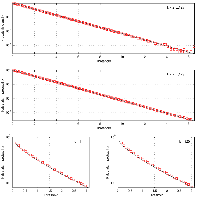
Figure 1: Probability density of the false alarm (upper plot) and the false alarm probability (middle plot) of 127 bins of the statistics ${\mathcal{F}}_{k}$ (for $k=2,\ldots,128$) given by Eq. (54). The false alarm probability of the first ($k=1$), zero frequency bin and the last ($k=129$), Nyquist frequency bin is given in the left lower and the right lower plot, respectively. The continuous lines in the upper and the middle plots are theoretical distributions given by Eqs. (31) and (33) for $n=2$ and the continuous lines in the lower plots are theoretical distributions that follow from the cumulative $\chi^{2}$ distribution with 1 degree of freedom. In the simulation one million of sequencies of 256 random independent samples drawn from zero mean and unit variance normal distribution were generated and modulus of their discrete Fourier transforms evaluated. The results of the simulations are marked by the squares.

where $|X_{k}|$ is the modulus of the $k$th component of the discrete Fourier transform of $x$. In other words the optimal statistics is the periodogram sampled at Fourier bins. When $x$ consists of independent identically distributed Gaussian random variables we know [17] that for $k=2,\ldots,N/2$ the statistics $2{\mathcal{F}}_{k}$ has a $\chi^{2}$ distribution with 2 degrees of freedom whereas for $k=1$ (zero frequency bin) and $k=N/2+1$ (maximum, Nyquist frequency bin) ${\mathcal{F}}_{k}$ has a $\chi^{2}$ distribution with 1 degree of freedom. In our Monte Carlo simulation we have generated the signal $10^{6}$ times and we have made histograms of 127 bins of the statistics ${\mathcal{F}}_{k}$. In the upper plot of Figure 1 we have shown the (appropriately normalized) histogram for all the Fourier bins for $k=2,\ldots,N/2$ and in the middle plot of Figure 1 we have presented the cumulative distribution. Thus the probability density generated in the upper plot is to be compared with Eq. (31) for $n=2$ whereas the distribution obtained in the middle one is to be compared with Eq. (33) for $n=2$. Both theoretical distributions are exponential and they are given by solid curves in the two plots. The last bin in the upper plot of Figure 1 deviates substantially from the exponential curve. This is because in this bin all the events above the maximum value of the histogram range are accumulated. We get $11$ events altogether in the last bin. The expected value of the events calculated from Eq. (43) is 8.25 (where we have put $N_{c}=127$). In the two lower plots of Figure 1 we have presented the cumulative distributions for the first and the last bin. The theoretical cumulative distribution that follows from the $\chi^{2}$ distribution with 1 degree of freedom is given by $1-\text{erf}(\sqrt{{\mathcal{F}}_{o}/2})$ (solid curve in the plots). We see that simulated and theoretical distributions agree very well.

We have next tested the formulae for the false alarm probabilities given by Eqs. (42) and (51) against the Monte Carlo simulations. We have considered again the case of $n=2$ and we have simulated the optimal statistics for the case of a monochromatic signal ($M=1$) and the case of a signal with one spindown included ($M=2$). We have generated the random sequence of length $N=2^{8}$ as in the first simulation described above. We have however introduced an extra parameter $P$—the zero padding. Namely we add zeros to the random sequence so that its total length is $(1+P)N$. When we take Fourier transform of the zero-padded signal we get additional points in the Fourier domain between the Fourier bins. Zero padding essentially amounts to interpolating the periodogram between the Fourier bins. Thus the larger the $P$ the closer the discretelly sampled periodogram to a continuous function. To generate the statistics ${\mathcal{F}}$ for the signal with one spindown we have multiplied the generated random sequence $x(k)$ by $T(k;l)=\exp[-2{\pi}il\sigma_{1}(k-1)^{2}]$, where $k=1,\ldots,N$, $l=10,\ldots,29$, and $\sigma_{1}=(3/\pi)\sqrt{5/2}$. The function $T(k;l)$ is called a filter or a template. The multiplication operation is the matched filtering which in our case is also called dechirping. The quantity $\sigma_{1}$ is the accuracy of estimation of the 1st spindown parameter for the optimal signal-to-noise ratio $d=1$ divided by $\sqrt{2}$ and it is the maximum extent of the ellipse defined by Eq. (38) measured from the origin along the spindown axis in the Cartesian (frequency, spindown)-plane. The parameter $\sigma_{1}$ defines the spacing of the templates that we choose in our simulations. The zero padding is always done after the dechirping operation. Our optimal statistics is the modulus of the discrete Fourier transform of the dechirped and zero padded data divided by the number of points in the original data ($2^{8}$ in our case). We have made $10^{5}$ trials.

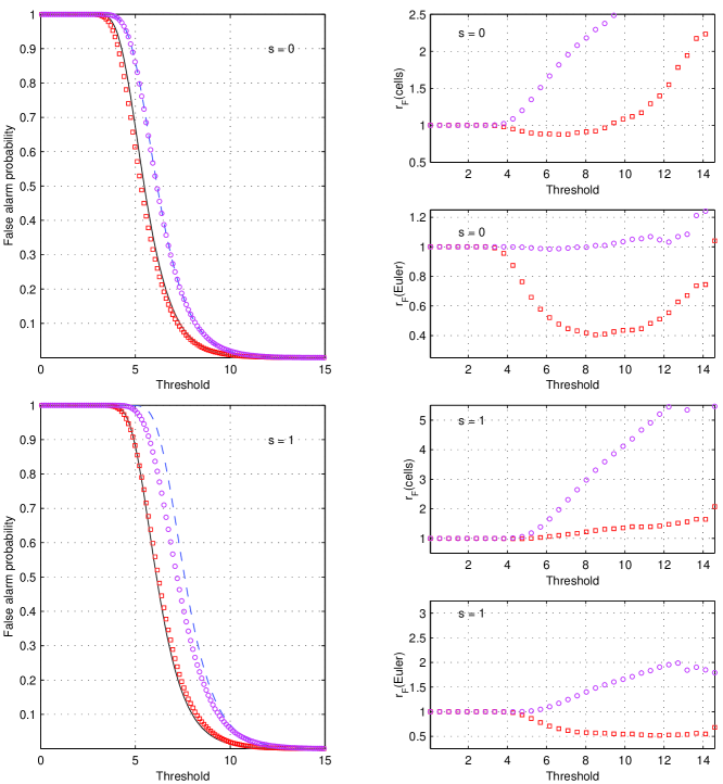
Figure 2: False alarm probabilities for a monochromatic (three upper plots) and a linearly frequency modulated signals (three lower plots). The same random sequences of length $N=2^{8}$ were generated as in the simulation in Figure 1 except that experiment was repeated $10^{5}$ times. The results of the simulation are marked by the squares (no zero padding) and by the circles (for the signal padded with $3N$ zeros). The ratio $r_{F}(\text{cells})$ is the quotient of the false alarm probability obtained from the simulations and calculated from Eq. (42) whereas $r_{F}(\text{Euler})$ is the quotient of the false alarm probability obtained from the simulations and calculated from Eq. (51).

The results of the simulation are presented in Figure 2. The three upper plots are the results for the monochromatic signal search and the three lower ones are the results for the one spindown signal search. The false alarm curves are given in the plots on the left. We see that the false alarm probability exhibits a threshold phenomenon, it drops very sharply within a narrow range of the detection threshold. We see from the plots on the left of Figure 2 that for $P=0$ (no zero padding) the results of the simulation agree well with Eq. (42) (solid line) whereas for $P=3$ there is a reasonable agreement with Eq. (51) (dashed line).

In the plots on the right of Figure 2 we have divided the probability of the false alarm obtained from the simulations by the probabilities obtained from the theoretical formulae. The upper plots give comparison with Eq. (42) based on dividing the parameter space into cells whereas the lower plots give comparison with Eq. (51) based on the expectation value of the Euler characteristic of the excursion set. We see that for the monochromatic signal for thresholds up to 10 Eq. (42) gives a reasonable agreement for $P=0$ whereas Eq. (51) gives a good agreement for $P=3$. For the frequency modulated signal for $P=0$ Eq. (42) underestimates the false alarm probability whereas Eq. (51) overestimates the false alarm probability. For $P=3$ there is an underestimate of the false alarm probability by both formulae. For thresholds greater than 10 the curves become irregular what may be attributed to a sparse number of events for such large thresholds.

3.3 Detection probability

When the signal is present a precise calculation of the pdf of ${\mathcal{F}}$ is very difficult because the presence of the signal makes the data random process $x(t)$ nonstationary. As a first approximation we can estimate the probability of detection of the signal when the parameters are unknown by the probability of detection when the parameters of the signal are known [given by Eq. (34)]. This approximation assumes that when the signal is present the true values of the phase parameters fall within the cell where ${\mathcal{F}}$ has a maximum. This approximation will be the better the higher the signal-to-noise ratio $d$. Parametric plot of probability of detection vs. probability of false alarm with optimal signal-to-noise ratio $d$ as a parameter is called the receiver operating characteristic (ROC).

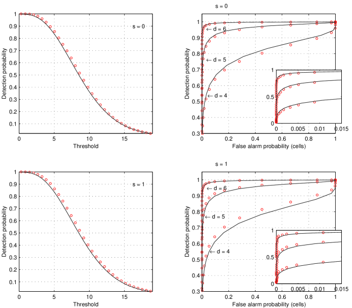
Figure 3: Probability of detection (plots on the left) and the receiver operating characteristic (plots on the right) for a monochromatic (upper plots) and a linearly frequency modulated signal (lower plots). The same random sequences of length $N=2^{8}$ were generated as in the simulation in Figure 1 except that the experiment was repeated $10^{4}$ times. The results of the simulation are marked by the circles. Theoretical distributions are given by solid lines. Probability of detection is calculated from Eqs. (32) and (34) for $n=2$ and optimal signal-to-noise ratio $d=4$. The receiver operating characteristics are parametric curves with signal-to-noise ratio $d$ as a parameter, they are calculated from Eqs. (34) and (42) for $d=4$, 5, and 6.

We have performed the numerical simulations to see how the ROC obtained from the analytical formulae presented above compares with that obtained from the discrete finite duration time series. We have generated the noise as in the simulations of the false alarm probability and we have added the signal. We have considered both the monochromatic and the linearly frequency modulated signal. The frequency of the signal was chosen not to coincide with one of the Fourier frequencies. However in the dechirping operation to detect the frequency modulated signal we have chosen the spindown parameter in the filter to coincide with the spindown parameter of the signal. We have perfomed $10^{4}$ trials and we have examined the cumulative distributions of the two Fourier bins between which the true value of the frequency of the signal had been chosen. The results are presented in Figure 3. The two upper plots are for the monochromatic signal and the lower two are for the one spindown signal. In the plots on the left we compare the probability of detection calculated from Eq. (34) with the results of the simulations and in the plots on the right we compare the theoretical and the simulated receiver operating characteristics. For the false alarm probability we have used the formula (42). In the inserts we have zoomed the ROC for small values of the false alarm probability. We see that the agreement between the theoretical and simulated ROC is quite good.

4 Number of cells for the one-component signal

Let us return to the case of a gravitational-wave signal from a spinning neutron star. In Sec. 5 of Paper II we have shown that each component of the $N$-component signal can be approximated by the following one-component signal:

$$h(t;h_{o},\Phi_{0},\boldsymbol{\xi})=h_{o}\sin\left[\Phi(t;\boldsymbol{\xi})+\Phi_{0}\right],$$ (55)

where the phase $\Phi$ of the signal is given by

$$\Phi(t;\boldsymbol{\xi}) = \sum_{k=0}^{s}\omega_{k}\left(\frac{t}{T_{o}}\right)^{k+1}+\frac{2\pi}{c}\left\{\alpha_{1}\left[R_{ES}\sin\left(\phi_{o}+\Omega_{o}t\right)+R_{E}\cos\lambda\cos\varepsilon\sin\left(\phi_{r}+\Omega_{r}t\right)\right]\right.$$ (56)

$$\left.+\alpha_{2}\left[R_{ES}\cos\left(\phi_{o}+\Omega_{o}t\right)+R_{E}\cos\lambda\cos\left(\phi_{r}+\Omega_{r}t\right)\right]\right\},$$

where $T_{o}$ denotes the observation time, $R_{ES}=$ 1 AU is the mean distance from the Earth’s center to the SSB, $R_{E}$ is the mean radius of the Earth, $\Omega_{o}$ is the mean orbital angular velocity of the Earth, and $\phi_{o}$ is a deterministic phase which defines the position of the Earth in its orbital motion at $t=0$, $\varepsilon$ is the angle between ecliptic and the Earth’s equator. The vector $\boldsymbol{\xi}$ collects all the phase parameters, it equals $\boldsymbol{\xi}=(\alpha_{1},\alpha_{2},\omega_{0},\ldots,\omega_{s})$, so the phase $\Phi$ depends on $s+3$ parameters. The dimensionless parameters $\omega_{k}$ are related to the spindown coefficients ${\stackrel{{\scriptstyle\scriptscriptstyle(k)}}{{f_{o}}}}$ introduced in Eq. (5) as follows:

$$\omega_{k}:=\frac{2\pi}{(k+1)!}{\stackrel{{\scriptstyle\scriptscriptstyle(k)}}{{f_{o}}}}T_{o}^{k+1},\quad k=0,\ldots,s.$$ (57)

The parameters $\alpha_{1}$ and $\alpha_{2}$ are defined by

$$\alpha_{1}:=f_{o}\left(\cos\varepsilon\sin\alpha\cos\delta+\sin\varepsilon\sin\delta\right),\quad\alpha_{2}:=f_{o}\cos\alpha\cos\delta.$$ (58)

In Appendix D we show that the parameters $\alpha_{1}$, $\alpha_{2}$ can be used instead of the parameters $\alpha$, $\delta$ to label the templates needed to do the matched filtering.

The signal defined by Eqs. (55) and (56) has two important properties: it has a constant amplitude and its phase is a linear function of the parameters $\boldsymbol{\xi}$. In Paper II we have shown that for this signal’s model the rms errors calculated from the inverse of the Fisher information matrix reproduce well the rms errors of the full model presented in Sec. 2. We will use here the simpified signal (55)–(56) to estimate the number of elementary cells in the parameter space.

For the signal given by Eqs. (55) and (56) the statistics ${\mathcal{F}}$ of Eq. (17) can be written as

$${\mathcal{F}}(\boldsymbol{\xi})\approx\frac{1}{2}\left\{[x_{c}(\boldsymbol{\xi})]^{2}+[x_{s}(\boldsymbol{\xi})]^{2}\right\},$$ (59)

where

$$x_{c}(\boldsymbol{\xi}):=2\sqrt{\frac{T_{o}}{S_{h}(f_{o})}}\left\langle x\cos\Phi(t;\boldsymbol{\xi})\right\rangle,\quad x_{s}(\boldsymbol{\xi}):=2\sqrt{\frac{T_{o}}{S_{h}(f_{o})}}\left\langle x\sin\Phi(t;\boldsymbol{\xi})\right\rangle.$$ (60)

We calculate the autocovariance function $C$ [defined by Eq. (36)] of the random field (59) when the data $x$ consists only of the noise $n$. We recall that $n$ is a zero mean stationary Gaussian random process. Consequently we have the following useful formulae [18]

$$\rm{E}\left\{(n|h_{1})(n|h_{2})\right\} = (h_{1}|h_{2}),$$ (61)

$$\rm{E}\left\{(n|h_{1})(n|h_{2})(n|h_{3})(n|h_{4})\right\} = (h_{1}|h_{2})(h_{3}|h_{4})+(h_{1}|h_{3})(h_{2}|h_{4})+(h_{1}|h_{4})(h_{2}|h_{3}),$$ (62)

where $h_{1}$, $h_{2}$, $h_{3}$, and $h_{4}$ are deterministic functions. Let us also observe that

$$\left\langle\sin^{2}\Phi(t;\boldsymbol{\xi})\right\rangle\approx\left\langle\cos^{2}\Phi(t;\boldsymbol{\xi})\right\rangle\approx\frac{1}{2}.$$ (63)

Making use of Eqs. (61), (62), and (63) one finds that

$$\rm{E}_{0}\left\{{\mathcal{F}}(\boldsymbol{\xi})\right\} \approx 1,$$ (64)

$$\rm{E}_{0}\left\{{\mathcal{F}}(\boldsymbol{\xi}){\mathcal{F}}(\boldsymbol{\xi}^{\prime})\right\} \approx 1+2\left[\left\langle\cos\Phi(t;\boldsymbol{\xi})\cos\Phi(t;\boldsymbol{\xi}^{\prime})\right\rangle^{2}+\left\langle\cos\Phi(t;\boldsymbol{\xi})\sin\Phi(t;\boldsymbol{\xi}^{\prime})\right\rangle^{2}\right.$$ (65)

$$\left.+\left\langle\sin\Phi(t;\boldsymbol{\xi})\cos\Phi(t;\boldsymbol{\xi}^{\prime})\right\rangle^{2}+\left\langle\sin\Phi(t;\boldsymbol{\xi})\sin\Phi(t;\boldsymbol{\xi}^{\prime})\right\rangle^{2}\right],$$

where subscript $0$ means that there is no signal in the data. For our narrowband signal to a good approximation we have

$$\left\langle\cos\Phi(t;\boldsymbol{\xi})\cos\Phi(t;\boldsymbol{\xi}^{\prime})\right\rangle \approx \frac{1}{2}\left\langle\cos[\Phi(t;\boldsymbol{\xi})-\Phi(t;\boldsymbol{\xi}^{\prime})]\right\rangle,$$ (66)

$$\left\langle\cos\Phi(t;\boldsymbol{\xi})\sin\Phi(t;\boldsymbol{\xi}^{\prime})\right\rangle \approx -\frac{1}{2}\left\langle\sin[\Phi(t;\boldsymbol{\xi})-\Phi(t;\boldsymbol{\xi}^{\prime})]\right\rangle,$$ (67)

$$\left\langle\sin\Phi(t;\boldsymbol{\xi})\cos\Phi(t;\boldsymbol{\xi}^{\prime})\right\rangle \approx \frac{1}{2}\left\langle\sin[\Phi(t;\boldsymbol{\xi})-\Phi(t;\boldsymbol{\xi}^{\prime})]\right\rangle,$$ (68)

$$\left\langle\sin\Phi(t;\boldsymbol{\xi})\sin\Phi(t;\boldsymbol{\xi}^{\prime})\right\rangle \approx \frac{1}{2}\left\langle\cos[\Phi(t;\boldsymbol{\xi})-\Phi(t;\boldsymbol{\xi}^{\prime})]\right\rangle.$$ (69)

Collecting Eqs. (64)–(69) together one gets

$$C(\boldsymbol{\xi},\boldsymbol{\xi}^{\prime}) = \rm{E}_{0}\left\{{\mathcal{F}}(\boldsymbol{\xi}){\mathcal{F}}(\boldsymbol{\xi}^{\prime})\right\}-\rm{E}_{0}\left\{{\mathcal{F}}(\boldsymbol{\xi})\right\}E_{0}\left\{{\mathcal{F}}(\boldsymbol{\xi}^{\prime})\right\}$$ (70)

$$\approx \left\langle\cos[\Phi(t;\boldsymbol{\xi})-\Phi(t;\boldsymbol{\xi}^{\prime})]\right\rangle^{2}+\left\langle\sin[\Phi(t;\boldsymbol{\xi})-\Phi(t;\boldsymbol{\xi}^{\prime})]\right\rangle^{2}.$$

The phase $\Phi$ given by Eq. (56) is a linear function of the parameters $\boldsymbol{\xi}$ hence the autocovariance function $C$ from Eq. (70) depends only on the difference $\boldsymbol{\tau}=\boldsymbol{\xi}-\boldsymbol{\xi}^{\prime}$ and it can be written as

$$C(\boldsymbol{\tau})\approx\left\langle\cos[\Phi(t;\boldsymbol{\tau})]\right\rangle^{2}+\left\langle\sin[\Phi(t;\boldsymbol{\tau})]\right\rangle^{2}.$$ (71)

To calculate the volume of the elementary cell by means of Eq. (40) we need to compute the matrix $G$ defined in Eq. (39). Substituting (71) into (39) we obtain

$$G=2\widetilde{\Gamma},$$ (72)

where the matrix $\widetilde{\Gamma}$ has the components

$$\widetilde{\Gamma}_{ij}:=\left\langle\frac{\partial\Phi}{\partial\tau_{i}}\frac{\partial\Phi}{\partial\tau_{j}}\right\rangle-\left\langle\frac{\partial\Phi}{\partial\tau_{i}}\right\rangle\left\langle\frac{\partial\Phi}{\partial\tau_{j}}\right\rangle.$$ (73)

The matrix $\widetilde{\Gamma}$ is the reduced Fisher information matrix for our signal where the initial phase parameter $\Phi_{0}$ [cf. Eq. (55)] has been reduced, see Appendix B.

As the mean (64) of the random field ${\mathcal{F}}$ is constant and its autocovariance (70) depends only on the difference $\boldsymbol{\xi}-\boldsymbol{\xi}^{\prime}$ the random field ${\mathcal{F}}$ is a homogeneous random field. Let us observe that for the fixed values of the parameters $\boldsymbol{\xi}$ the random variables $x_{c}$ and $x_{s}$ are zero mean and unit variance Gaussian random variables. However the correlation between the Gaussian fields $x_{c}$ and $x_{s}$ does not vanish:

$$\rm{E}\left\{x_{c}(\boldsymbol{\xi})x_{s}(\boldsymbol{\xi}^{\prime})\right\}\approx\left\langle\sin[\Phi(t;\boldsymbol{\xi})-\Phi(t;\boldsymbol{\xi}^{\prime})]\right\rangle,$$ (74)

and thus the Gaussian random fields $x_{c}$ and $x_{s}$ are not independent. Therefore ${\mathcal{F}}$ is not a $\chi^{2}$ random field but only a generalized $\chi^{2}$ random field. Our formula for the number of cells [Eq. (41)] and the formula for the false alarm probability [Eq. (42)] apply to any homogeneous random fields however formula (47) applies only to $\chi^{2}$ fields. Nevertheless by examining the proof of formula (47) [13, 16] we find that it is very likely that the formula holds for generalized $\chi^{2}$ random fields as well if we replace the determinant of the matrix $\Lambda$ by the determinant of the reduced Fisher matrix $\widetilde{\Gamma}$.

The total volume of the parameter space depends on the range of the individual parameters. Following Ref. [7] we assume that

$$2\pi T_{o}f_{\text{min}}\leq\omega_{0}\leq 2\pi T_{o}f_{\text{max}},$$ (75)

$$-\beta_{k}\omega_{0}\leq\omega_{k}\leq\beta_{k}\omega_{0},\quad\text{where}\quad\beta_{k}:={\displaystyle\frac{1}{k+1}\left(\frac{T_{o}}{\tau_{\text{min}}}\right)^{k}},\quad k=1,\ldots,s,$$ (76)

where $f_{\text{min}}$ and $f_{\text{max}}$ are respectively the minimum and the maximum value of the gravitational-wave frequency, $\tau_{\text{min}}$ is the minimum spindown age of the neutron star. The parameters $\alpha_{1}$ and $\alpha_{2}$ defined in Eq. (58) fill, for the fixed value of the frequency parameter $\omega_{0}$, 2-dimensional ball concentrated around the origin in the $(\alpha_{1},\alpha_{2})$-plane, with radius equal to $\omega_{0}/(2\pi T_{o})$:

$$(\alpha_{1},\alpha_{2})\in B_{2}(0,\omega_{0}/(2\pi T_{o})).$$ (77)

Taking Eqs. (75)–(77) into account the total volume $V_{\text{total}(s)}^{\text{all}}$ of the parameter space for all-sky searches with $s$ spindowns included can be calculated as follows

$$V_{\text{total}(s)}^{\text{all}} = \int\limits_{2\pi T_{o}f_{\text{min}}}^{2\pi T_{o}f_{\text{max}}}d\,\omega_{0}{\int\!\!\int}_{B_{2}(0,\omega_{0}/(2\pi T_{o}))}d\,\alpha_{1}\,d\,\alpha_{2}\int\limits_{-\beta_{1}\omega_{0}}^{\beta_{1}\omega_{0}}d\,\omega_{1}\ldots\int\limits_{-\beta_{s}\omega_{0}}^{\beta_{s}\omega_{0}}d\,\omega_{s}$$ (78)

$$= \frac{2^{2s+1}\pi^{s+2}}{(s+3)(s+1)!}T_{o}^{s+1}\left(\frac{T_{o}}{\tau_{\text{min}}}\right)^{s(s+1)/2}\left(f_{\text{max}}^{s+3}-f_{\text{min}}^{s+3}\right).$$

The volume $V_{\text{cell}(s)}^{\text{all}}$ of one cell we calculate from Eq. (40) for $M=s+3$ and $G=2\widetilde{\Gamma}_{(s)}^{\text{all}}$, where $\widetilde{\Gamma}_{(s)}^{\text{all}}$ is the reduced Fisher matrix (73) for the phase $\Phi$ given by Eq. (56) with $s$ spindowns included:

$$V_{\text{cell}(s)}^{\text{all}}=\frac{(\pi/2)^{(s+3)/2}}{\Gamma((s+5)/2)\sqrt{\det\widetilde{\Gamma}_{(s)}^{\text{all}}}}.$$ (79)

In Appendix B we have given formulae needed to calculate matrices $\widetilde{\Gamma}_{(s)}^{\text{all}}$ for $s=0,\ldots,4$ analytically. In Figure 4 we have plotted the volume $V_{\text{cell}(s)}^{\text{all}}$ of one cell as a function of the observation time for signals with various numbers $s$ of spindown parameters included.

The number $N_{\text{cells}(s)}^{\text{all}}$ of cells for all-sky searches is given by

$$N_{\text{cells}(s)}^{\text{all}}=\frac{V_{\text{total}(s)}^{\text{all}}}{V_{\text{cell}(s)}^{\text{all}}}=\frac{2^{(3s+1)/2}\pi^{s/2+1}}{\Gamma(s/2+1)}\sqrt{\det\widetilde{\Gamma}_{(s)}^{\text{all}}}\left(\frac{T_{o}}{\tau_{\text{min}}}\right)^{s(s+1)/2}T_{o}^{s+1}\left(f_{\text{max}}^{s+3}-f_{\text{min}}^{s+3}\right).$$ (80)

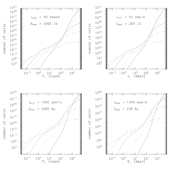
Figure 5: Number of cells in all-sky searches as a function of the observation time $T_{o}$ for different values of the minimum spindown age $\tau_{\text{min}}$ and the maximum gravitational-wave frequency $f_{\text{max}}$ (the minimum gravitational-wave frequency $f_{\text{min}}=0$). The lines shown in the plots correspond to different numbers $s$ of spindowns included: $s=4$ (solid), $s=3$ (dotted), $s=2$ (dashed), $s=1$ (dotted/dashed), and $s=0$ (double dotted/dashed). We have assumed the LIGO Hanford detector and we have put $\phi_{r}=1.456$ and $\phi_{o}=0.123$.

In Figure 5 we have plotted the number $N_{\text{cells}(s)}^{\text{all}}$ of cells as a function of the observation time $T_{o}$ for various models of the signal depending on the minimum spindown age $\tau_{\text{min}}$ and the maximum gravitational-wave frequency $f_{\text{max}}$, and for various numbers $s$ of spindowns included (the minimum gravitational-wave frequency $f_{\text{min}}=0$). We see that for a given $\tau_{\text{min}}$ and $f_{\text{max}}$ curves corresponding to different numbers $s$ intersect. This effect was observed and explained by Brady et al. [7]. To obtain the number of cells for a given observation time $T_{o}$ we always take the number of cells given by the uppermost curve. We have calculated the observation times $T_{\text{cross}(k)}^{\text{all}}$ for which the numbers of cells with $k$ and $k+1$ spindowns included coincide:

$$N_{\text{cells}(k+1)}^{\text{all}}(T_{o}=T_{\text{cross}(k)}^{\text{all}})=N_{\text{cells}(k)}^{\text{all}}(T_{o}=T_{\text{cross}(k)}^{\text{all}}),\quad k=0,\ldots,s-1.$$ (81)

In Table 1 we have given the values of $T_{\text{cross}(k)}^{\text{all}}$ for all the signal models considered.

$\tau_{\text{min}}$ (years)	$f_{\text{max}}$ (Hz)	$T_{\text{cross}(k)}^{\text{all}}$ (days)				$T_{\text{cross}(k)}^{\text{dir}}$ (days)
		$k=0$	$k=1$	$k=2$	$k=3$	$k=0$	$k=1$	$k=2$	$k=3$
40	$10^{3}$	0.21	3.11	116	311	0.03	3.53	40.5	175
40	200	0.31	5.19	158	389	0.06	6.04	60.5	242
$10^{3}$	$10^{3}$	0.46	114	575	2210	0.14	30.2	452	2300
$10^{3}$	200	0.69	157	725	3040	0.32	51.7	676	3180

Table 1: The observation times for which the numbers of cells with $k$ and $k+1$ spindowns included coincide for various models of the signal depending on the minimum spindown age $\tau_{\text{min}}$ and the maximum gravitational-wave frequency $f_{\text{max}}$. The minimum gravitational-wave frequency $f_{\text{min}}=0$. In the case of all-sky searches we have used the latitude $\lambda=46.45^{\circ}$ of the LIGO Hanford detector and we have put $\phi_{o}=0.123$ and $\phi_{r}=1.456$.

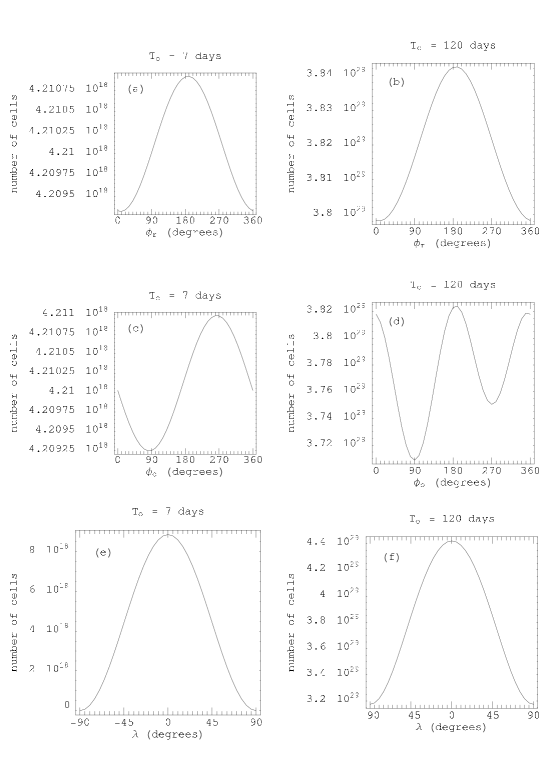
Figure 6: Dependence of number of cells in all-sky searches on the angles $\phi_{r}$, $\phi_{o}$, and the latitude $\lambda$ of the detector’s site. We have chosen the minimum spindown age $\tau_{\text{min}}=40$ years, the maximum gravitational-wave frequency $f_{\text{max}}=1$ kHz, and the minimum gravitational-wave frequency $f_{\text{min}}=0$. The plots (a), (c), and (e) are for the observation time $T_{o}$ = 7 days (and the number of spindowns $s=2$); (b), (d), and (f) are for $T_{o}$ = 120 days (and the number of spindowns $s=3$). In the plots (a), (b), (c), (d) we have used the latitude $\lambda=46.45^{\circ}$ of the LIGO Hanford detector; in (a), (b), (e), (f) we have put $\phi_{o}=0.123$; and in (c), (d), (e), (f) we have used $\phi_{r}=1.456$.

The Fisher matrix $\widetilde{\Gamma}_{(s)}^{\text{all}}$ depends on the phases $\phi_{r}$, $\phi_{o}$, and the latitude $\lambda$ of the detector (see Appendix B). We know from Paper II (see Appendix C of Paper II) that the Fisher matrix also depends on the choice of the instant of time at which the instantanenous frequency and spindown parameters are defined (in the present paper this moment is chosen to coincide with the middle of the observational interval). We find that the determinant $\det\widetilde{\Gamma}_{(s)}^{\text{all}}$ and consequently the number of cells does not depend on this choice. The dependence on the remaining parameters is studied in Figure 6. The dependence on the phases $\phi_{r}$ and $\phi_{o}$ is quite weak. The dependence on $\lambda$ is quite strong however for the detectors under construction for which $\lambda$ varies from $35.68^{\circ}$ (TAMA300) to $52.25^{\circ}$ (GEO600) the number of cells changes by a factor of 2 for 7 days of observation time and by around 10% for 120 days of observation time.

In Sec. 5 of Paper II we have shown that for directed searches the constant amplitude signal given by Eqs. (55) and (56) can be further simplified by discarding in the phase (56) terms due to the motion of the detector w.r.t. the SSB and the rms errors calculated form the inverse of the Fisher matrix do not change substancially. Such a signal reads

$$h(t;h_{o},\Phi_{0},\boldsymbol{\xi})=h_{o}\sin\left[\Phi(t;\boldsymbol{\xi})+\Phi_{0}\right],\quad\Phi(t;\boldsymbol{\xi})=\sum_{k=0}^{s}\omega_{k}\left(\frac{t}{T_{o}}\right)^{k+1}.$$ (82)

The vector $\boldsymbol{\xi}$ has now $s+1$ components: $\boldsymbol{\xi}=(\omega_{0},\ldots,\omega_{s})$.

Using Eqs. (75) and (76) the total volume $V_{\text{total}(s)}^{\text{dir}}$ of the parameter space with $s$ spindowns included for directed searches is calculated as follows

$$V_{\text{total}(s)}^{\text{dir}} = \int\limits_{2\pi T_{o}f_{\text{min}}}^{2\pi T_{o}f_{\text{max}}}d\,\omega_{0}\int\limits_{-\beta_{1}\omega_{0}}^{\beta_{1}\omega_{0}}d\,\omega_{1}\ldots\int\limits_{-\beta_{s}\omega_{0}}^{\beta_{s}\omega_{0}}d\,\omega_{s}$$ (83)

$$= \frac{2^{2s+1}\pi^{s+1}}{(s+1)(s+1)!}T_{o}^{s+1}\left(\frac{T_{o}}{\tau_{\text{min}}}\right)^{s(s+1)/2}\left(f_{\text{max}}^{s+1}-f_{\text{min}}^{s+1}\right).$$

The volume $V_{\text{total}(s)}^{\text{dir}}$ of one cell we calculate from Eq. (40) for $M=s+1$ and $G=2\widetilde{\Gamma}_{(s)}^{\text{dir}}$, where $\widetilde{\Gamma}_{(s)}^{\text{dir}}$ is the reduced Fisher matrix (73) for the polynomial phase (82) with $s$ spindowns included:

$$V_{\text{cell}(s)}^{\text{dir}}=\frac{(\pi/2)^{(s+1)/2}}{\Gamma((s+3)/2)\sqrt{\det\widetilde{\Gamma}_{(s)}^{\text{dir}}}}.$$ (84)

The matrix $\widetilde{\Gamma}_{(s)}^{\text{dir}}$ for $s=0,\ldots,4$ can be calculated analytically by means of formulae given in Appendix B.

The number $N_{\text{cells}(s)}^{\text{dir}}$ of independent cells is given by

$$N_{\text{cells}(s)}^{\text{dir}}=\frac{V_{\text{total}(s)}^{\text{dir}}}{V_{\text{cell}(s)}^{\text{dir}}}=\frac{2^{(3s+1)/2}\pi^{s/2+1}}{(s+1)\Gamma(s/2+1)}\sqrt{\det\widetilde{\Gamma}_{(s)}^{\text{dir}}}\left(\frac{T_{o}}{\tau_{\text{min}}}\right)^{s(s+1)/2}T_{o}^{s+1}\left(f_{\text{max}}^{s+1}-f_{\text{min}}^{s+1}\right).$$ (85)

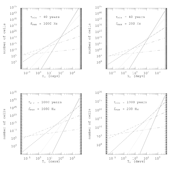
Figure 7: Number of cells in directed searches as a function of the observation time $T_{o}$ for different values of the minimum spindown age $\tau_{\text{min}}$ and the maximum gravitational-wave frequency $f_{\text{max}}$ (the minimum gravitational-wave frequency $f_{\text{min}}=0$). The lines shown in the plots correspond to different numbers $s$ of spindowns included: $s=4$ (solid), $s=3$ (dotted), $s=2$ (dashed), $s=1$ (dotted/dashed), and $s=0$ (double dotted/dashed).

In Figure 7 we have plotted the number of cells $N_{\text{cells}(s)}^{\text{dir}}$ as a function of the observation time $T_{o}$ for various models of the signal depending on the minimum spindown age $\tau_{\text{min}}$, the maximum gravitational-wave frequency $f_{\text{max}}$, and the number $s$ of spindowns included (the minimum gravitational-wave frequency $f_{\text{min}}=0$). We see that like for all-sky searches for a given $\tau_{\text{min}}$ and $f_{\text{max}}$ curves corresponding to different numbers $s$ intersect. We have calculated analytically the observation times $T_{\text{cross}(k)}^{\text{dir}}$ for which the numbers of cells with $k$ and $k+1$ spindowns included coincide:

$$N_{\text{cells}(k+1)}^{\text{dir}}\left(T_{o}=T_{\text{cross}(k)}^{\text{dir}}\right)=N_{\text{cells}(k)}^{\text{dir}}\left(T_{o}=T_{\text{cross}(k)}^{\text{dir}}\right),\quad k=0,\ldots,s-1.$$ (86)

Using Eq. (85) one obtains

$$T_{\text{cross}(k)}^{\text{dir}}=\left[\frac{(k+2)\Gamma((k+3)/2)}{2\sqrt{2\pi}(k+1)\Gamma((k+2)/2)}\sqrt{\frac{\det\widetilde{\Gamma}_{(k)}^{\text{dir}}}{\det\widetilde{\Gamma}_{(k+1)}^{\text{dir}}}}\frac{f_{\text{max}}^{k+1}-f_{\text{min}}^{k+1}}{f_{\text{max}}^{k+2}-f_{\text{min}}^{k+2}}\tau_{\text{min}}^{k+1}\right]^{1/(k+2)},\quad k=0,\ldots,s-1.$$ (87)

In Table 1 we have given the values of $T_{\text{cross}(k)}^{\text{dir}}$ for all the signal models considered.

In Table 2 we have given the number of cells both for all-sky and directed searches for various models of the signal depending on the minimum spindown age $\tau_{\text{min}}$ and the maximum gravitational-wave frequency $f_{\text{max}}$, and for the observation time $T_{o}$ of 7 and 120 days (the minimum gravitational-wave frequency $f_{\text{min}}=0$). The number of cells is calculated from Eq. (80) for all-sky searches and from Eq. (85) in the case of directed searches. For a given observation time $T_{o}$ the number $s$ of spindowns one should include in the signal’s model is obtained as such number $s$ chosen out of $s=0,\ldots,4$ for which $N_{\text{cells}(s)}^{\text{all}}$ (or $N_{\text{cells}(s)}^{\text{dir}}$) is the greatest.

We have also calculated the threshold ${\mathcal{F}}_{o}$ for the $1\%$ false alarm probability (or equivalently for $99\%$ detection confidence). By means of Eqs. (33) and (42) for $n=2$ (what corresponds to a one-component signal) the relation between the threshold ${\mathcal{F}}_{o}$ and the false alarm probability $\alpha$ reads

$${\mathcal{F}}_{o}=-\ln\left[1-(1-\alpha)^{1/N_{c}}\right],\quad\alpha=0.01,$$ (88)

where $N_{c}$ is the number of cells. Following the relation between the expectation value of the optimum statistics when the signal is present and the signal-to-noise ratio which is given by

$$\rm{E}_{1}\{{\mathcal{F}}\}=1+\frac{1}{2}d^{2},$$ (89)

we have calculated the ”threshold” signal-to-noise ratio

$$d_{o}:=\sqrt{2({\mathcal{F}}_{o}-1)},$$ (90)

where ${\mathcal{F}}_{o}$ is given by Eq. (88). The values of $d_{o}$ for various models of the signal and observation times of 7 and 120 days are given in Table 2. If the signal-to-noise ratio is $d_{o}$ then there is roughly a $50\%$ probability that the optimum statistic will cross the threshold ${\mathcal{F}}_{o}$.

$T_{o}$ (days)	$\tau_{\text{min}}$ (years)	$f_{\text{max}}$ (Hz)	all-sky			directed
			$s$	$N_{\text{cells}(s)}^{\text{all}}$	$d_{o}$	$s$	$N_{\text{cells}(s)}^{\text{dir}}$	$d_{o}$
7	40	$10^{3}$	2	$4.2\times 10^{18}$	9.6	2	$3.7\times 10^{14}$	8.6
7	40	200	2	$1.3\times 10^{15}$	8.8	2	$2.9\times 10^{12}$	8.0
7	$10^{3}$	$10^{3}$	1	$1.5\times 10^{16}$	9.0	1	$1.9\times 10^{12}$	8.0
7	$10^{3}$	200	1	$2.4\times 10^{13}$	8.3	1	$7.6\times 10^{10}$	7.6
120	40	$10^{3}$	3	$3.8\times 10^{29}$	12	3	$7.2\times 10^{23}$	11
120	40	200	2	$1.1\times 10^{26}$	11	3	$1.2\times 10^{21}$	10
120	$10^{3}$	$10^{3}$	2	$2.2\times 10^{25}$	11	2	$6.0\times 10^{17}$	9.4
120	$10^{3}$	200	1	$2.7\times 10^{22}$	11	2	$4.8\times 10^{15}$	8.9

Table 2: Number of cells for all-sky and directed searches for various models of the signal depending on the minimum spindown age $\tau_{\text{min}}$ and the maximum gravitational-wave frequency $f_{\text{max}}$, and for the observation time $T_{o}$ of 7 and 120 days. The minimum gravitational-wave frequency $f_{\text{min}}=0$. To calculate the Fisher matrix $\widetilde{\Gamma}_{(s)}^{\text{all}}$ we have used the latitude $\lambda=46.45^{\circ}$ of the LIGO Hanford detector and we have put $\phi_{o}=0.123$ and $\phi_{r}=1.456$. For each case we also give the $99\%$ confidence threshold signal-to-noise ratio $d_{o}$ calculated by virtue of Eq. (90).

5 Number of filters for the one-component signal

To calculate the number of FFTs to do the search we first need to calculate the volume of the elementary cell in the subspace of the parameter space defined by $\omega_{0}=$ const. This subspace of the parameter space is called the filter space.

Let us expand the autocovariance function $C$ of Eq. (71) around $\boldsymbol{\tau}=0$ up to terms of second order in $\boldsymbol{\tau}$:

$$C\left(\boldsymbol{\tau}\right)=1-\sum_{i,j=1}^{M}\widetilde{\Gamma}_{ij}\tau_{i}\tau_{j},$$ (91)

where $\widetilde{\Gamma}_{ij}$ are defined in Eq. (73) and $M$ is the number of phase parameters. In Eq.  (91) we have used the property that $C$ attains its maximum value of 1 for $\boldsymbol{\tau}=0$. Let us assume that $\tau_{1}$ corresponds to frequency parameter and let us maximize $C$ given by Eq. (91) with respect to $\tau_{1}$. It is easy to show that $C$ attains its maximum value, keeping $\tau_{2}$, …, $\tau_{M}$ fixed, for

$${\overline{\tau}}_{1}=-\frac{1}{\Gamma_{11}}\sum_{i=2}^{M}\Gamma_{1i}\tau_{i}.$$ (92)

Let us define

$${\overline{C}}\left(\tau_{2},\ldots,\tau_{M}\right):=C\left({\overline{\tau}}_{1},\tau_{2},\ldots,\tau_{M}\right).$$ (93)

Substituting Eqs. (91) and (92) into Eq. (93) we obtain

$${\overline{C}}\left(\tau_{2},\ldots,\tau_{M}\right)=1-\sum_{i,j=2}^{M}\overline{\Gamma}_{ij}\tau_{i}\tau_{j},$$ (94)

where

$$\overline{\Gamma}_{ij}:=\widetilde{\Gamma}_{ij}-\frac{\widetilde{\Gamma}_{1i}\widetilde{\Gamma}_{1j}}{\widetilde{\Gamma}_{11}}.$$ (95)

We define an elementary cell in the filter space by the requirement that at the boundary of the cell the correlation $\overline{C}$ equals 1/2:

$${\overline{C}}\left(\tau_{2},\ldots,\tau_{M}\right)=\frac{1}{2}.$$ (96)

Substituting (94) into (96) we arrive at the equation describing the surface of the elementary hyperellipsoid in the filter space:

$$\sum_{i,j=2}^{M}\overline{\Gamma}_{ij}\tau_{i}\tau_{j}=\frac{1}{2}.$$ (97)

The volume of the elementary cell is thus equal to [cf. Eq. (40)]

$$\overline{V}_{\text{cell}}=\frac{(\pi/2)^{(M-1)/2}}{\Gamma((M+1)/2)\sqrt{\det\overline{\Gamma}}}.$$ (98)

The volume $\overline{V}_{\text{cell}}$ of the elementary cell in the filter space is independent on the value of the frequency parameter.

Taking Eqs. (75)–(77) into account the total volume $\overline{V}_{\text{total}(s)}^{\text{all}}$ of the filter space for all-sky searches with $s$ spindowns included can be calculated as follows

$$\overline{V}_{\text{total}(s)}^{\text{all}} = \left\{{\int\!\!\int}_{B_{2}(0,\omega_{0}/(2\pi T_{o}))}d\,\alpha_{1}\,d\,\alpha_{2}\int\limits_{-\beta_{1}\omega_{0}}^{\beta_{1}\omega_{0}}d\,\omega_{1}\ldots\int\limits_{-\beta_{s}\omega_{0}}^{\beta_{s}\omega_{0}}d\,\omega_{s}\right\}_{\omega_{0}=2\pi T_{o}f_{\text{max}}}$$ (99)

$$= \frac{2^{2s}\pi^{s+1}}{(s+1)!}T_{o}^{s}\left(\frac{T_{o}}{\tau_{\text{min}}}\right)^{s(s+1)/2}f_{\text{max}}^{s+2}.$$ (100)

Putting in Eq. (99) $\omega_{0}=2\pi T_{o}f_{\text{max}}$ we have defined $\overline{V}_{\text{total}(s)}^{\text{all}}$ as that slice $\omega_{0}=\textit{const}$ of the parameter space which has maximum volume.

The volume $\overline{V}_{\text{cell}(s)}^{\text{all}}$ of one cell in the filter space we calculate from Eq. (98) for $M=s+3$:

$$\overline{V}_{\text{cell}(s)}^{\text{all}}=\frac{(\pi/2)^{(s+2)/2}}{\Gamma((s+4)/2)\sqrt{\det\overline{\Gamma}_{(s)}^{\text{all}}}},$$ (101)

where the matrix $\overline{\Gamma}_{(s)}^{\text{all}}$ is calulated from Eq. (95) for $\widetilde{\Gamma}=\widetilde{\Gamma}_{(s)}^{\text{all}}$.

The number $N_{\text{filters}(s)}^{\text{all}}$ of filters for all-sky searches is given by

$$N_{\text{filters}(s)}^{\text{all}}=\frac{\overline{V}_{\text{total}(s)}^{\text{all}}}{\overline{V}_{\text{cell}(s)}^{\text{all}}}=\frac{2^{3s/2}\pi^{(s+1)/2}(s+2)}{(s+1)\Gamma((s+1)/2)}\sqrt{\det\overline{\Gamma}_{(s)}^{\text{all}}}\left(\frac{T_{o}}{\tau_{\text{min}}}\right)^{s(s+1)/2}T_{o}^{s}f_{\text{max}}^{s+2}.$$ (102)

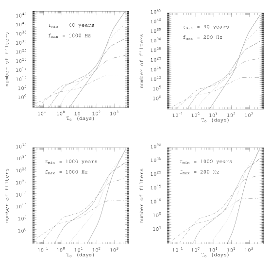
Figure 8: Number of filters in all-sky searches as a function of the observation time $T_{o}$ for different values of the minimum spindown age $\tau_{\text{min}}$ and the maximum gravitational-wave frequency $f_{\text{max}}$. The lines shown in the plots correspond to different numbers $s$ of spindowns included: $s=4$ (solid), $s=3$ (dotted), $s=2$ (dashed), $s=1$ (dotted/dashed), and $s=0$ (double dotted/dashed). We have assumed the LIGO Hanford detector and we have put $\phi_{r}=1.456$ and $\phi_{o}=0.123$.

In Figure 8 we have plotted the number $N_{\text{filters}(s)}^{\text{all}}$ of filters as a function of the observation time $T_{o}$ for various models of the signal depending on the minimum spindown age $\tau_{\text{min}}$ and the maximum gravitational-wave frequency $f_{\text{max}}$, and for various numbers $s$ of spindowns included. We see that for a given $\tau_{\text{min}}$ and $f_{\text{max}}$ curves corresponding to different numbers $s$ intersect. This effect was observed and explained in Ref. [7]: in the regime where adding an extra parameter reduces the number of filters the parameter space in the extra dimension extends less than the width of the elementary cell in this dimension. To obtain the number of filters for a given observation time $T_{o}$ we always take the number of filters given by the uppermost curve. We have also calculated the observation times $\overline{T}_{\text{cross}(k)}^{\text{all}}$ for which the numbers of filters with $k$ and $k+1$ spindowns included coincide:

$$N_{\text{filters}(k+1)}^{\text{all}}(T_{o}=\overline{T}_{\text{cross}(k)}^{\text{all}})=N_{\text{filters}(k)}^{\text{all}}(T_{o}=\overline{T}_{\text{cross}(k)}^{\text{all}}),\quad k=0,\ldots,s-1.$$ (103)

In Table 3 we have given the values of $\overline{T}_{\text{cross}(k)}^{\text{all}}$ for all the signal models considered.

$\tau_{\text{min}}$ (years)	$f_{\text{max}}$ (Hz)	$\overline{T}_{\text{cross}(k)}^{\text{all}}$ (days)				$\overline{T}_{\text{cross}(k)}^{\text{dir}}$ (days)
		$k=0$	$k=1$	$k=2$	$k=3$	$k=1$	$k=2$	$k=3$
40	$10^{3}$	0.19	3.01	113	307	3.26	38.8	171
40	200	0.30	5.07	156	384	5.58	58.0	236
$10^{3}$	$10^{3}$	0.45	111	566	2170	27.9	434	2250
$10^{3}$	200	0.66	153	715	2990	47.7	649	3100

Table 3: The observation times for which the numbers of filters with $k$ and $k+1$ spindowns included coincide for various models of the signal depending on the minimum spindown age $\tau_{\text{min}}$ and the maximum gravitational-wave frequency $f_{\text{max}}$. In the case of all-sky searches we have used the latitude $\lambda=46.45^{\circ}$ of the LIGO Hanford detector and we have put $\phi_{o}=0.123$ and $\phi_{r}=1.456$.

For directed searches the total volume $\overline{V}_{\text{total}(s)}^{\text{dir}}$ of the filter space with $s$ spindowns included we calculate using Eqs. (75) and (76):

$$\overline{V}_{\text{total}(s)}^{\text{dir}}=\left\{\int\limits_{-\beta_{1}\omega_{0}}^{\beta_{1}\omega_{0}}d\,\omega_{1}\ldots\int\limits_{-\beta_{s}\omega_{0}}^{\beta_{s}\omega_{0}}d\,\omega_{s}\right\}_{\omega_{0}=2\pi T_{o}f_{\text{max}}}=\frac{2^{2s}\pi^{s}}{(s+1)!}\left(\frac{T_{o}}{\tau_{\text{min}}}\right)^{s(s+1)/2}\left(f_{\text{max}}T_{o}\right)^{s}.$$ (104)

The volume $\overline{V}_{\text{cell}(s)}^{\text{dir}}$ of one cell in the filter space for directed searches with $s$ spindowns included we calculate from Eq. (98) for $M=s+1$:

$$\overline{V}_{\text{cell}(s)}^{\text{dir}}=\frac{(\pi/2)^{s/2}}{\Gamma((s+2)/2)\sqrt{\det\overline{\Gamma}_{(s)}^{\text{dir}}}},$$ (105)

where the matrix $\overline{\Gamma}_{(s)}^{\text{dir}}$ is calulated from Eq. (95) for $\widetilde{\Gamma}=\widetilde{\Gamma}_{(s)}^{\text{dir}}$.

The number $N_{\text{filters}(s)}^{\text{all}}$ of filters in the case of directed searches is thus given by:

$$N_{\text{filters}(s)}^{\text{dir}}=\frac{\overline{V}_{\text{total}(s)}^{\text{dir}}}{\overline{V}_{\text{cell}(s)}^{\text{dir}}}=\frac{2^{(3s-2)/2}\pi^{(s+1)/2}}{\Gamma((s+3)/2)}\sqrt{\det\overline{\Gamma}_{(s)}^{\text{dir}}}\left(\frac{T_{o}}{\tau_{\text{min}}}\right)^{s(s+1)/2}\left(f_{\text{max}}T_{o}\right)^{s}.$$ (106)

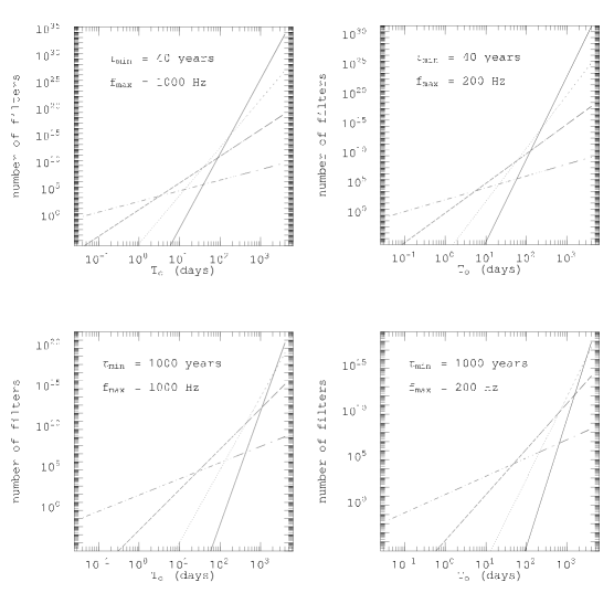
Figure 9: Number of filters in directed searches as a function of the observation time $T_{o}$ for different values of the minimum spindown age $\tau_{\text{min}}$ and the maximum gravitational-wave frequency $f_{\text{max}}$. The lines shown in the plots correspond to different numbers $s$ of spindowns included: $s=4$ (solid), $s=3$ (dotted), $s=2$ (dashed), $s=1$ (dotted/dashed).

In Figure 9 we have plotted the number of filters for various models of the signal depending on the minimum spindown age $\tau_{\text{min}}$ and the maximum gravitational-wave frequency $f_{\text{max}}$, and for various numbers $s$ of spindowns included. We have also calculated analytically the observation times $\overline{T}_{\text{cross}(k)}^{\text{dir}}$ for which the numbers of filters with $k$ and $k+1$ spindowns included coincide:

$$N_{\text{filters}(k+1)}^{\text{dir}}\left(T_{o}=\overline{T}_{\text{cross}(k)}^{\text{dir}}\right)=N_{\text{filters}(k)}^{\text{dir}}\left(T_{o}=\overline{T}_{\text{cross}(k)}^{\text{dir}}\right),\quad k=1,\ldots,s-1.$$ (107)

Using Eq. (106) one obtains

$$\overline{T}_{\text{cross}(k)}^{\text{dir}}=\left[\frac{\Gamma((k+4)/2)}{2\sqrt{2\pi}\Gamma((k+3)/2)}\sqrt{\frac{\det\overline{\Gamma}^{\text{dir}}_{(k)}}{\det\overline{\Gamma}^{\text{dir}}_{(k+1)}}}\frac{\tau_{\text{min}}^{k+1}}{f_{\text{max}}}\right]^{1/(k+2)},\quad k=1,\ldots,s-1.$$ (108)

In Table 3 we have given the values of $\overline{T}_{\text{cross}(k)}^{\text{dir}}$ for all the signal models considered.

In Table 4 we have given the number of filters both for all-sky and directed searches for various models of the signal depending on the minimum spindown age $\tau_{\text{min}}$ and the maximum gravitational-wave frequency $f_{\text{max}}$, and for the observation time $T_{o}$ of 7 and 120 days. The number of filters is calculated from Eq. (102) for all-sky searches and from Eq. (106) in the case of directed searches. For a given observation time $T_{o}$ the number $s$ of spindowns one should include in the signal’s model is obtained as such number $s$ chosen out of $s=0,\ldots,4$ for which $N_{\text{filters}(s)}^{\text{all}}$ (or $N_{\text{filters}(s)}^{\text{dir}}$) is the greatest.

$T_{o}$ (days)	$\tau_{\text{min}}$ (years)	$f_{\text{max}}$ (Hz)	all-sky			directed
			$s$	$N_{\text{filters}(s)}^{\text{all}}$	${\mathcal{P}}$ (Tf)	$s$	$N_{\text{filters}(s)}^{\text{dir}}$	${\mathcal{P}}$ (Tf)
7	40	$10^{3}$	2	$1.4\times 10^{10}$	$2.6\times 10^{3}$	2	$9.5\times 10^{5}$	$1.7\times 10^{-1}$
7	40	200	2	$2.3\times 10^{7}$	$7.8\times 10^{-1}$	2	$3.8\times 10^{4}$	$1.3\times 10^{-3}$
7	$10^{3}$	$10^{3}$	1	$4.6\times 10^{7}$	8.5	1	$3.8\times 10^{3}$	$7.0\times 10^{-4}$
7	$10^{3}$	200	1	$3.7\times 10^{5}$	$1.3\times 10^{-2}$	1	$7.7\times 10^{2}$	$2.6\times 10^{-5}$
120	40	$10^{3}$	3	$8.4\times 10^{19}$	$1.7\times 10^{13}$	3	$1.3\times 10^{14}$	$2.7\times 10^{7}$
120	40	200	2	$1.1\times 10^{17}$	$4.3\times 10^{9}$	3	$1.0\times 10^{12}$	$3.9\times 10^{4}$
120	$10^{3}$	$10^{3}$	2	$4.4\times 10^{15}$	$9.2\times 10^{8}$	2	$9.0\times 10^{7}$	$1.8\times 10$
120	$10^{3}$	200	1	$2.4\times 10^{13}$	$9.3\times 10^{5}$	2	$3.6\times 10^{6}$	$1.4\times 10^{-1}$

Table 4: Number of filters for all-sky and directed searches for various models of the signal depending on the minimum spindown age $\tau_{\text{min}}$ and the maximum gravitational-wave frequency $f_{\text{max}}$, and for the observation time $T_{o}$ of 7 and 120 days. To calculate the Fisher matrix $\overline{\Gamma}_{(s)}^{\text{all}}$ we have used the latitude $\lambda=46.45^{\circ}$ of the LIGO Hanford detector and we have put $\phi_{o}=0.123$ and $\phi_{r}=1.456$. For each case we also give the number ${\mathcal{P}}$ of floating point operations per second (flops) needed to do the search; ${\mathcal{P}}$ is calculated by means of Eq. (109).

We shall next compare the number of filters obtained above with the number of filters calculated by Brady et al. [7]. In their calculations they have assumed a constant amplitude of the signal however they have used a full model of the phase. To calculate the number of templates they have used so called metric approach of Owen [19]. They have assumed a certain geometry of spacing of the templates: combination of a hexagonal and a hypercubic spacing and they have introduced an additional parameter—a mismatch $\mu$, which was the measure of the correlation of the two neighbouring templates. Also in their calculation they have assumed that the data processing method involves resampling of the time series so that the resampled signal is monochromatic. We shall compare the number of filters in Table 4 of our paper with the corresponding number of filters given in Table 1 of [7]. Our calculations correspond to mismatch $\mu=0.5$. This means that to compare our numbers of filters with the corresponding numbers of Brady et al. our numbers have to be multiplied by 2.4, 5.8, 15, and 40 for the signal with 0, 1, 2, and 3 spindowns respectively for all-sky searches and by 1.3, 1.7, 2.2 for 1, 2, and 3 spindowns respectively for directed searches. The difference in the volume of our hyperellipsoidal cells and their volumes of elementary patches means [see Ref. [7], Eq. (5.18) for all-sky searches and the paragraph above Eq. (7.2) for directed searches] that our numbers aditionally have to be multiplied by 1.7, 2.2, 2.8, and 3.6 for all-sky searches and by 1.0, 1.4, 1.3 for directed searches for comparison. After introducing the corrections for the mismatch parameter and the size of an elementary cell we find that our corrected number of templates is greater than the number of templates given in Table 1 of [7] by (going from top to bottom of Table 1) $2.8\times 10^{4}$, 14, 2.7, and 1.5 for all-sky searches and by 2.2, 1.7, 0.31, and 0.25 for directed searches. We thus conclude that considering the differences in the way the calculations were done there is a reasonable agreement between the number of filters obtained by the two approaches except for one case: all-sky searches with the maximum frequency $f_{\text{max}}=200$ Hz and the minimum spindown age $\tau_{\text{min}}=1000$ years where the difference is 4 orders of magnitude.

We would also like to point out to the uncertainties in the calculation of the number of filters. Our model of the intrinsic spin frequency evolution of the neutron star is extremely simple: we approximate the frequency evolution by a Taylor series. In reality the frequency evolution will be determined by complex physical processes. The size of the parameter space is likewise uncertain. The range for the spindown parameters [see Eqs. (75)–(76)] was chosen so that the total size of our parameter space is the same as in [7]. The approximation of the time derivative of the frequency as $f_{\text{max}}/\tau_{\text{min}}$ that is used to estimate the maximum value of the spindowns is probably an order of magnitude estimate. This implies that the size of the parameter space and consequently the number of filters is accurate within $s(s+1)/2$ orders of magnitude, where $s$ is the number of spindowns in the phase of the signal. Even this large uncertainty does not change the conclusion that all-sky searches for 120 days of observation time are computationally too prohibitive.

To estimate the computational requirement to do the signal search we adopt a simple formula [see Eq. (6.11) of [7]] for the number ${\mathcal{P}}$ of floating point operations per second (flops) required assuming that the data processing rate should be comparable to the data aquisition rate (it is assumed that fast Fourier transform (FFT) algorithm is used):

$${\mathcal{P}}=6f_{\text{max}}N_{f}[\log_{2}(2f_{\text{max}}T_{o})+1/2],$$ (109)

where $N_{f}$ is the number of filters. The above formula assumes that we calculate only one modulus of the Fourier transform. Calculation of the optimal statistics ${\mathcal{F}}$ for the amplitude modulated signal requires two such muduli for each component of the signal [see Eq. (99) of Paper I, we assume that the observation time is an integer multiple of the sidereal day so that $C=0$] and several multiplications. Moreover if dechirping operations are used instead of resampling, the data processing would involve complex FFTs. All these operation will not increase the complexity of the analysis i.e. the number of floating point operations will still go as $O(N\log_{2}(N))$, where $N$ is the number of points to be processed.

In Table 4 we have given the computer power ${\mathcal{P}}$ (in Teraflops, Tf) required for all the cases considered. We see that for 120 days of observation time all-sky searches are computationally too prohibitive whereas for directed searches only one case ($\tau_{\text{min}}=1000$ years, $f_{\text{max}}=200$ Hz) is within reach of a 1 Teraflops computer. For 7 days of observation time all cases except for the most demanding all-sky search with $\tau_{\text{min}}=40$ years and $f_{\text{max}}=1$ kHz are within a reach of a 1 Teraflops computer.

Finally we would like to point to a technique that can distribute the data processing into several smaller computers. We shall call this technique signal splitting. We can divide the available bandwidth of the detector $(f_{\text{min}},f_{\text{max}})$ into $M$ adjacent intervals of length $B$. We then apply a standard technique of heterodyning. For each of the chosen bands we multiply our data time series by $\exp(-2\pi if_{I})$, where $f_{I}=f_{\text{min}}+IB$ ($I=0,\ldots,M-1$). Such an operation moves the spectrum of the data towards zero by frequency $f_{I}$. We then apply a low pass filter with a cutoff frequency $B$ and we resample the resulting sequence with the frequency $2B$. The result is $M$ time series sampled at frequency $2B$ instead of one sampled at $2f_{\text{max}}$. The resampled sequencies are shorter than the original ones by a factor of $M$ and each can be processed by a separate computer. We only need to perform the signal splitting operation once before the signal search. The splitting operation can also be performed continuously when the data are collected so that there is no delay in the analysis. The signal splitting does not lead to a substancial saving in the total computational power but yields shorter data sequencies for the analysis. For example for the case of 7 days of observation time and sampling rate of 1 kHz the data itself would occupy around 10 GB of memory (assuming double precision) which is available on expensive supercomputers whereas if we split the data into a bandwidth of 50 Hz so that sampling frequency is only 100 Hz each sequence will occupy 0.5 GB memory which is available on inexpensive personal computers.

In the case of a narrowband detector, e.g. for the GEO600 detector tuned to a certain frequency $f_{o}$ around a bandwidth $B$, it is natural to apply the above data reduction technique so that the resulting sampling frequency is $2B$. Such a technique is applied in data preprocessing of bar detectors [23]. From the formulae given in the present section one can show that to perform the all-sky search with the integration time of 7 days for pulsars in the bandwidth of 50 Hz around the frequency of 300 Hz and minimum spindown age of 40 years so that the processing proceeds at the rate of data aquisition requires a 1 Teraflops computer. Since the data sequence occupies only 0.5 GB of memory the data processing task can be distributed over several smaller computers. If we also relax the requirement of data processing to be done in real time the signal search can be performed by a 20 Gigaflops workstation in a year.

6 Suboptimal filtering

It will very often be the case that the filter we use to extract the signal from the noise is not optimal. This may be the case when we do not know the exact form of the signal (this is almost always the case in practice) or we choose a suboptimal filter to reduce the computational cost and simplify the analysis. We shall consider here an important special case of a suboptimal filter that may be usful in the analysis of gravitational-wave signals from a spinning neutron star.

6.1 General theory

We shall assume a constant amplitude one-component model of the signal. Then the optimal (maximum likelihood) statistics is given by Eq. (59). Let us suppose that we do not model the phase accurately and instead of the two optimal filters $\cos\left[\Phi(t;\boldsymbol{\xi})\right]$ and $\sin\left[\Phi(t;\boldsymbol{\xi})\right]$ we use filters with a phase $\Phi^{\prime}(t;\boldsymbol{\xi}^{\prime})$, where function $\Phi^{\prime}$ is different form $\Phi$ and the set of filter parameters $\boldsymbol{\xi}^{\prime}$ is in general different from $\boldsymbol{\xi}$, i.e. ${\mathcal{F}}_{\text{sub}}$ has the form [cf. Eqs. (59) and (60)]

$${\mathcal{F}}_{\text{sub}}=\frac{2T_{o}}{S_{h}(f_{o})}\left[\left\langle x\cos\Phi^{\prime}(t;\boldsymbol{\xi}^{\prime})\right\rangle^{2}+\left\langle x\sin\Phi^{\prime}(t;\boldsymbol{\xi}^{\prime})\right\rangle^{2}\right],$$ (110)

where we have assumed that the suboptimal filters are narrowband at some ”carrier” frequency $f_{o}$ as in the case of optimal filters.

Let us first establish the probability density functions of ${\mathcal{F}}_{\text{sub}}$ when the phase parameters $\boldsymbol{\xi}^{\prime}$ are known. Since the dependence on the data random process is the same as in the optimal case the false alarm and detection probability densities will be the same as for the optimal case i.e. $2{\mathcal{F}}_{\text{sub}}$ has a central or a noncentral $\chi^{2}$ distribution with 2 degrees of freedom depending on whether the signal is absent or present. From the narrowband property of the suboptimal filter we get the following expressions for the expectation values and the variances of ${\mathcal{F}}_{\text{sub}}$ ($0$ means that signal is absent and $1$ means that signal is present):

$$\text{E}_{0}\left\{{\mathcal{F}}_{\text{sub}}\right\}=1,\quad\text{E}_{1}\left\{{\mathcal{F}}_{\text{sub}}\right\}=1+\frac{1}{2}d_{\text{sub}}^{2},$$ (111)

$$\text{Var}_{0}\left\{{\mathcal{F}}_{\text{sub}}\right\}=1,\quad\text{Var}_{1}\left\{{\mathcal{F}}_{\text{sub}}\right\}=1+d_{\text{sub}}^{2},$$ (112)

where

$$d_{\text{sub}}:=d\left\{\left\langle\cos[\Phi(t;\boldsymbol{\xi})-\Phi^{\prime}(t;\boldsymbol{\xi}^{\prime})]\right\rangle^{2}+\left\langle\sin[\Phi(t;\boldsymbol{\xi})-\Phi^{\prime}(t;\boldsymbol{\xi}^{\prime})]\right\rangle^{2}\right\}^{1/2},$$ (113)

here $d$ is the optimal signal-to-noise ratio.

We see that for the suboptimal filter introduced above the false alarm probability has exactly the same $\chi^{2}$ distribution as in the optimal case whereas the probability of detection has noncentral $\chi^{2}$ distribution but with a different noncentrality parameter $d_{\text{sub}}^{2}$. We shall call $d_{\text{sub}}$ (the square root of the noncentrality parameter) the suboptimal signal-to-noise ratio. It is clear that when the phases of the signal and the suboptimal filter are different the suboptimal signal-to-noise ratio is strictly less and the probability of detection is less than for the optimal filter.

When the parameters $\boldsymbol{\xi}^{\prime}$ are unknown the functional ${\mathcal{F}}_{\text{sub}}$ is a random field and we can obtain the false alarm probabilities as in the case of an optimal filter. Here we only quote the formula based on the number of independent cells of the random field. One thing we must remember is that the number of cells for the suboptimal and the optimal filters will in general be different because they may have a different functional dependence and a different number of parameters. Thus we have [cf. Eqs. (33) and (42) for $n=2$]

$$P^{T}_{sF}({\mathcal{F}}_{o})=1-[1-\exp(-{\mathcal{F}}_{o})]^{N_{sc}},$$ (114)

where $N_{sc}$ is the number of cells for the suboptimal filter.

The detection probability for the suboptimal filter is given by [cf. Eqs. (32) and (34) for $n=2$]

$$P_{sD}(d_{\text{sub}},{\mathcal{F}}_{o}):=\int^{\infty}_{{\mathcal{F}}_{o}}p_{s1}(d_{\text{sub}},{\mathcal{F}})\,d{\mathcal{F}},$$ (115)

where

$$p_{s1}({d_{\text{sub}},{\mathcal{F}}})=I_{0}\left(d_{\text{sub}}\sqrt{2{\mathcal{F}}}\right)\exp\left(-{\mathcal{F}}-\frac{1}{2}d_{\text{sub}}^{2}\right).$$ (116)

Probability of detection for the suboptimal filter is obtained from the probability of detection for the optimal one by replacing the optimal signal-to-noise ratio $d$ by the suboptimal one $d_{\text{sub}}$.

When we design a suboptimal filtering scheme we would like to know what is the expected number of false alarms with such a scheme and what is the expected number of detections. As in the optimal case the expected number $N_{sF}$ of false alarms with suboptimal filter is given by [cf. Eqs. (33) and (43) for $n=2$]

$$N_{sF}=N_{sc}\exp(-{\mathcal{F}}_{o}).$$ (117)

To obtain the expected number of detections we assume that the signal-to-noise ratio $d$ varies inversely proportionally to the distance from the source and that the sources are uniformly distributed in space. We also assume that the space is Euclidean. Let us denote by $d_{1}$ the signal-to-noise ratio for which the number of events is one. Then the number of events corresponding to the signal-to-noise ratio $d$ is $(d_{1}/d)^{3}$. The expected number of the detected events is given by

$$N_{D}(d_{1},{\mathcal{F}}_{o})=3\int^{\infty}_{0}x^{2}P_{D}\left(\frac{d_{1}}{x},{\mathcal{F}}_{o}\right)\,dx$$ (118)

in the case of the optimal filter, and by

$$N_{sD}(d_{1\text{sub}},{\mathcal{F}}_{o})=3\int^{\infty}_{0}x^{2}P_{sD}\left(\frac{d_{1\text{sub}}}{x},{\mathcal{F}}_{o}\right)\,dx$$ (119)

for the suboptimal filter. Let us note that [cf. Eq. (113)]

$$d_{1\text{sub}}=d_{1}\left\{\left\langle\cos[\Phi(t;\boldsymbol{\xi})-\Phi^{\prime}(t;\boldsymbol{\xi}^{\prime})]\right\rangle^{2}+\left\langle\sin[\Phi(t;\boldsymbol{\xi})-\Phi^{\prime}(t;\boldsymbol{\xi}^{\prime})]\right\rangle^{2}\right\}^{1/2}.$$ (120)

Because of the statistical nature of the detection any signal can only be detected with a certain probability less than 1. In the case of Gaussian noise for signals with the signal-to-noise ratio around the threshold this probability is roughly 1/2 and it increases exponentially with increasing signal-to-noise ratio. In Appendix C we give a worked example of the application of the statistical formulae for the suboptimal filtering derived above.

6.2 Fitting factor

To study the quality of suboptimal filters (or search templates as they are sometimes called) one of the present authors [20, 21] introduced an $l-$factor defined as the square root of the correlation between the signal and the suboptimal filter. It turned out that a more general and more natural quantity is the fitting factor introduced by Apostolatos [22]. The fitting factor FF between a signal $h(t;\boldsymbol{\theta})$ and a filter $h^{\prime}(t;\boldsymbol{\theta}^{\prime})$ ($\boldsymbol{\theta}$ and $\boldsymbol{\theta}^{\prime}$ are the parameters of the signal and the filter, respectively) is defined as

$$\text{FF}:=\max_{\boldsymbol{\theta}^{\prime}}\frac{\left(h(t;\boldsymbol{\theta})|h^{\prime}(t;\boldsymbol{\theta}^{\prime})\right)}{\sqrt{\left(h(t;\boldsymbol{\theta})|h(t;\boldsymbol{\theta})\right)}\sqrt{\left(h^{\prime}(t;\boldsymbol{\theta}^{\prime})|h^{\prime}(t;\boldsymbol{\theta}^{\prime})\right)}}.$$ (121)

If both the signal $h$ and the filter $h^{\prime}$ are narrowband around the same frequency $f_{o}$ the scalar products $(\cdot|\cdot)$ from Eq. (121) can be computed from the formula

$$(h_{1}|h_{2})\approx\frac{2}{S_{h}(f_{o})}\int_{-T_{o}/2}^{T_{o}/2}h_{1}(t)h_{2}(t)\,dt,$$ (122)

where $S_{h}$ is the one-sided noise spectral density and $T_{o}$ is the observation time.

Let us assume that the signal and the filter can be written as

$$h(t;\boldsymbol{\theta})=h_{o}\sin\Psi(t;\boldsymbol{\zeta}),\quad h^{\prime}(t;\boldsymbol{\theta}^{\prime})=h^{\prime}_{o}\sin\Psi^{\prime}(t;\boldsymbol{\zeta}^{\prime}),$$ (123)

where $h_{o}$ and $h^{\prime}_{o}$ are constant amplitudes, $\boldsymbol{\zeta}$ and $\boldsymbol{\zeta}^{\prime}$ denote the parameters entering the phases $\Psi$ and $\Psi^{\prime}$ of the signal and the filter, respectively. We substitute Eqs. (123) into Eq. (121). Using Eq. (122) we obtain

$$\text{FF}\approx\max_{\boldsymbol{\zeta}^{\prime}}\frac{1}{T_{o}}\int_{-T_{o}/2}^{T_{o}/2}\cos\left[\Psi(t;\boldsymbol{\zeta})-\Psi^{\prime}(t;\boldsymbol{\zeta}^{\prime})\right]\,dt.$$ (124)

It is easy to maximize the FF (124) with respect to the initial phase of the filter. Let us denote the initial phases of the functions $\Psi$ and $\Psi^{\prime}$ by $\Phi_{0}$ and $\Phi^{\prime}_{0}$, respectively. Then

$$\Psi(t;\boldsymbol{\zeta})=\Phi(t;\boldsymbol{\xi})+\Phi_{0},\quad\Psi^{\prime}(t;\boldsymbol{\zeta}^{\prime})=\Phi^{\prime}(t;\boldsymbol{\xi}^{\prime})+\Phi^{\prime}_{0},$$ (125)

where $\boldsymbol{\xi}$ and $\boldsymbol{\xi}^{\prime}$ denote the remaining parameters of the signal and the filter, respectivley. After substitution Eqs. (125) into Eq. (124) we easily get

FF $$\approx \max_{\Phi^{\prime}_{0},\boldsymbol{\xi}^{\prime}}\left\langle\cos\left[\Phi(t;\boldsymbol{\xi})-\Phi^{\prime}(t;\boldsymbol{\xi}^{\prime})+\left(\Phi_{0}-\Phi^{\prime}_{0}\right)\right]\right\rangle$$ (126)

$$= \max_{\Phi^{\prime}_{0},\boldsymbol{\xi}^{\prime}}\left\{\cos\left(\Phi_{0}-\Phi^{\prime}_{0}\right)\left\langle\cos\left[\Phi(t;\boldsymbol{\xi})-\Phi^{\prime}(t;\boldsymbol{\xi}^{\prime})\right]\right\rangle-\sin\left(\Phi_{0}-\Phi^{\prime}_{0}\right)\left\langle\sin\left[\Phi(t;\boldsymbol{\xi})-\Phi^{\prime}(t;\boldsymbol{\xi}^{\prime})\right]\right\rangle\right\}$$

$$= \max_{\boldsymbol{\xi}^{\prime}}\left\{\left\langle\cos\left[\Phi(t;\boldsymbol{\xi})-\Phi^{\prime}(t;\boldsymbol{\xi}^{\prime})\right]\right\rangle^{2}+\left\langle\sin\left[\Phi(t;\boldsymbol{\xi})-\Phi^{\prime}(t;\boldsymbol{\xi}^{\prime})\right]\right\rangle^{2}\right\}^{1/2}.$$

Thus we obtain that the FF is nothing else but the ratio of the maximized value of the suboptimal signal-to-noise ratio $d_{\text{sub}}$ and the optimal signal-to-noise ratio $d$ [cf. Eq. (113)]. We stress however that the value of the fitting factor by itself is not adequate for determining the quality of a particular search template—one also needs the underlying probability distributions (both the false alarm and the detection) derived in the previous subsection. This is clearly shown by an example in Appendix C.

In the remaining part of this subsection we shall propose a way of approximate computation of the fitting factor. Let us now assume that the filter and the signal coincide, i.e. $\Phi^{\prime}=\Phi$, and the filter parameters $\boldsymbol{\xi}^{\prime}$ differ from the parameters $\boldsymbol{\xi}$ of the signal by small quantities $\Delta\boldsymbol{\xi}$: $\boldsymbol{\xi}^{\prime}=\boldsymbol{\xi}+\Delta\boldsymbol{\xi}$. The Eq. (126) can be rewritten as

$$\text{FF}\approx\max_{\Delta\boldsymbol{\xi}}\left\{\left\langle\cos\left[\Phi(t;\boldsymbol{\xi})-\Phi(t;\boldsymbol{\xi}+\Delta\boldsymbol{\xi})\right]\right\rangle^{2}+\left\langle\sin\left[\Phi(t;\boldsymbol{\xi})-\Phi(t;\boldsymbol{\xi}+\Delta\boldsymbol{\xi})\right]\right\rangle^{2}\right\}^{1/2}.$$ (127)

Obviously the FF (127) attains its maximum value of 1 when $\Delta\boldsymbol{\xi}=0$. Let us expand the expression in curly brackets on the right-hand side of Eq. (127) w.r.t. $\Delta\boldsymbol{\xi}$ around $\Delta\boldsymbol{\xi}=0$ up to terms of second order in $\Delta\boldsymbol{\xi}$. The result is

$$\text{FF}\approx\left\{1-\min_{\Delta\boldsymbol{\xi}}\left(\sum_{i,j}\Gamma_{ij}\Delta\xi_{i}\Delta\xi_{j}\right)\right\}^{1/2},$$ (128)

where

$$\Gamma_{ij}:=\left\langle\frac{\partial\Phi}{\partial\xi_{i}}\frac{\partial\Phi}{\partial\xi_{j}}\right\rangle-\left\langle\frac{\partial\Phi}{\partial\xi_{i}}\right\rangle\left\langle\frac{\partial\Phi}{\partial\xi_{j}}\right\rangle.$$ (129)

One can employ the formula (128) to estimate the FF in the case when the filter $\Phi^{\prime}$ is obtained from the signal $\Phi$ by replacing some of the signal parameters by zeros, provided the signal $\Phi$ depends weakly on these discarded parameters. Let the signal $\Phi$ depend on $n$ parameters $\xi_{1},\ldots,\xi_{n}$, and the filter $\Phi^{\prime}$ is defined by

$$\Phi^{\prime}(t;\xi^{\prime}_{1},\ldots,\xi^{\prime}_{k}):=\Phi(t;\xi^{\prime}_{1},\ldots,\xi^{\prime}_{k},\underbrace{0,\ldots,0}_{n-k}),$$ (130)

where $k<n$, so the filter $\Phi^{\prime}$ depends on $k$ parameters $\xi^{\prime}_{1},\ldots,\xi^{\prime}_{k}$. One can write

$$\Phi(t;\boldsymbol{\xi})-\Phi^{\prime}(t;\boldsymbol{\xi}^{\prime})=\Phi(t;\xi_{1},\ldots,\xi_{n})-\Phi(t;\xi^{\prime}_{1},\ldots,\xi^{\prime}_{k},\underbrace{0,\ldots,0}_{n-k})=\Phi(t;\boldsymbol{\xi})-\Phi(t;\boldsymbol{\xi}+\Delta\boldsymbol{\xi})$$ (131)

with

$$\Delta\xi_{i}=\left\{\begin{array}[]{ll}\xi^{\prime}_{i}-\xi_{i},&i=1,\ldots,k,\\ -\xi_{i},&i=k+1,\ldots,n.\end{array}\right.$$ (132)

We want to approximate the differnce $\Phi(t;\boldsymbol{\xi})-\Phi(t;\boldsymbol{\xi}+\Delta\boldsymbol{\xi})$ with $\Delta\boldsymbol{\xi}$ given by Eq. (132) by its Taylor expansion around $\Delta\boldsymbol{\xi}=0$. It is reasonable provided the two following conditions are satisfied. Firstly, the filter parameters differ slightly from the respective parameters of the signal, i.e. the quantitites $\Delta\xi_{i}$ are small compared to $\xi_{i}$ for $i=1,\ldots,k$. Secondly, the function $\Phi$ depends on the parameters $\xi_{k+1},\ldots,\xi_{n}$ (discarded from the filter) weakly enough to make a reasonable approximation by Taylor expansion up to $\Delta\xi_{i}=-\xi_{i}$ for $i=k+1,\ldots,n$. If the above holds, one can use the formula (128) to approximate the FF. Taking Eqs. (131) and (132) into account, from Eq. (128) one gets

$$\text{FF}\approx\left\{1-\min_{\Delta\xi_{1},\ldots,\Delta\xi_{k}}\left(\sum_{i,j=1}^{n}\Gamma_{ij}\Delta\xi_{i}\Delta\xi_{j}\Bigg{|}_{\Delta\xi_{k+1}=-\xi_{k+1},\ldots,\Delta\xi_{n}=-\xi_{n}}\right)\right\}^{1/2}.$$ (133)

6.3 Fitting factor vs. 1/4 of a cycle criterion

Let us consider the phase of the gravitational-wave signal of the form [cf. Eq. (5)]

$$\Phi(t)=2\pi\sum_{k=0}^{s_{1}}{\stackrel{{\scriptstyle\scriptscriptstyle(k)}}{{f_{o}}}}\frac{t^{k+1}}{(k+1)!}+\frac{2\pi}{c}{\bf n}_{0}\cdot{\bf r}_{\rm ES}(t)\sum_{k=0}^{s_{2}}{\stackrel{{\scriptstyle\scriptscriptstyle(k)}}{{f_{o}}}}\frac{t^{k}}{k!}+\frac{2\pi}{c}{\bf n}_{0}\cdot{\bf r}_{\rm E}(t)\sum_{k=0}^{s_{3}}{\stackrel{{\scriptstyle\scriptscriptstyle(k)}}{{f_{o}}}}\frac{t^{k}}{k!}.$$ (134)

In Paper I we have introduced the following criterion: we exclude an effect from the model of the signal in the case when it contributes less than 1/4 of a cycle to the phase of the signal during the observation time. In Paper II we have shown that if we restrict to observation times $T_{o}\leq 120$ days, frequencies $f_{o}\leq 1000$ Hz, and spindown ages $\tau\geq 40$ years, the phase model (134) meets the criterion for an appropriate choice of the numbers $s_{1}$, $s_{2}$, and $s_{3}$. We have also shown that the effect of the star proper motion in the phase is negligible if we assume that the star moves w.r.t. the SSB not faster than $10^{3}$ km/s and its distance to the Earth $r_{o}\geq 1$ kpc. In Table 5, which is Table 1 of Paper II, one can find the numbers $s_{1}$, $s_{2}$, and $s_{3}$ needed to meet 1/4 of a cycle criterion for different observation times $T_{o}$, maximum values $f_{\text{max}}$ of the gravitational-wave frequency, and minimum values $\tau_{\text{min}}$ of the neutron star spindown age.

$T_{o}$ (days)	$\tau_{\text{min}}$ (years)	$f_{\text{max}}$ (Hz)	$s_{1}$	$s_{2}$	$s_{3}$
120	40	$10^{3}$	4	3	0
120	40	200	4	2	0
120	$10^{3}$	$10^{3}$	2	1	0
120	$10^{3}$	200	2	1	0
7	40	$10^{3}$	2	1	0
7	40	200	2	1	0
7	$10^{3}$	$10^{3}$	1	1	0
7	$10^{3}$	200	1	1	0

Table 5: The number of spindown terms needed in various contributions to the phase of the signal depending on the type of population of neutron stars searched for [cf. Eq. (134)]. The number $s_{1}$ refers to the dominant polynomial in time term in Eq. (134), $s_{2}$ refers to the Earth orbital motion contribution, and $s_{3}$ refers to the Earth diurnal motion contribution.

In Appendix A of Paper I we have indicated that the 1/4 of a cycle criterion is only a sufficient condition to exclude a parameter from the phase of the signal but not necessary. In this subsection we study the effect of neglecting certain parameters in the template by calculating FFs. We employ the approximate formula (133) developed in the previous subsection to calculate FF between the one-component constant amplitude signals with the phases given by Eq. (134) for numbers $s_{1}$, $s_{2}$, and $s_{3}$ taken from Table 5 and the same signals with a smaller number (as compared to that given in Table 5) of spindowns included. We have found that for the first two models of Table 5 if in the template one neglects the fourth spindown, FF is greater than 0.99, both for all-sky and directed searches. For other cases in Table 5 we have found that neglecting any spindown parameter can result in the FF appreciably less than one.

In Paper II we have considered the effect of the proper motion of the neutron star on the phase of the signal assuming that it moves uniformly with respect to the SSB reference frame. We have found that for the observation time $T_{o}=$ 120 days and the extreme case of a neutron star at a distance $r_{o}=$ 40 pc moving with the transverse velocity $|{\bf v}_{{\rm ns}\perp}|=10^{3}$ km/s (where ${\bf v}_{{\rm ns}\perp}$ is the component of the star’s velocity ${\bf v}_{\rm ns}$ perpendicular to the vector ${\bf n}_{0}$), gravitational-wave frequency $f_{o}=1$ kHz, and spindown age $\tau=$ 40 years, proper motion contributes only $\sim$4 cycles to the phase of the signal. We have shown in Paper II that in this extreme case the phase model consistent with the 1/4 of a cycle criterion reads [cf. Eq. (33) in Paper II]

$$\Phi(t)=2\pi\sum_{k=0}^{4}{\stackrel{{\scriptstyle\scriptscriptstyle(k)}}{{f_{o}}}}\frac{t^{k+1}}{(k+1)!}+\frac{2\pi}{c}{\bf n}_{0}\cdot{\bf r}_{\rm ES}(t)\sum_{k=0}^{3}{\stackrel{{\scriptstyle\scriptscriptstyle(k)}}{{f_{o}}}}\frac{t^{k}}{k!}+\frac{2\pi}{c}\left({\bf n}_{0}\cdot{\bf r}_{\rm E}(t)+\frac{{\bf v}_{{\rm ns}\perp}}{r_{o}}\cdot{\bf r}_{\rm ES}(t)\,t\right)f_{o}.$$ (135)

The ratio ${\bf v}_{{\rm ns}\perp}/r_{o}$ determines the proper motion of the star and can be expressed in terms of the proper motions $\mu_{\alpha}$ and $\mu_{\delta}$ in right ascension $\alpha$ and declination $\delta$, respectively (see Sec. 4 of Paper II).

For the extreme case described above we have applied formula (133) to calculate the FF between the one-component constant amplitude signal with the phase given by Eq. (135) and the same signal with a simplified phase. We have found that when both proper motion parameteres $\mu_{\alpha}$, $\mu_{\delta}$ and the fourth spindown parameter ${\stackrel{{\scriptstyle\scriptscriptstyle(4)}}{{f_{o}}}}$ are neglected, the FF is greater than 0.99 for both all-sky and directed searches. Thus we conclude that neglecting the fourth spindown and the proper motion does not reduce appreciably the probability of detection of the signal.

It is also interesting to compare the results obtained from the calculation of the fitting factor with the results summarized in Table 1 for the observation times when the number of cells for models with $k$ and $k+1$ spindowns coincides. The observation times given in Table 1 can be interpreted as observation times at which one should include the $k+1$ parameter in the template. We see that for the first two models in Table 5 the Table 1 says that only 3 spindowns are needed as indicated by the calculation of the FF. The remaining cases also agree except for the cases of 120 days of observation time and 200 Hz frequency where Table 1 indicates one less spindown than Table 5. Finally we note that the crossover observation times in Table 1 agree within a few percent with those for the number of filters given in Table 3.

7 Monte Carlo simulations and the Cramér-Rao bound

As signal-to-noise ratio goes to infinity the maximum-liklihood estimators become unbiased and their rms errors tend to the errors calculated from the covariance matrix. The rms errors calculated from the covariance matrix are the smallest error achievable for unbiased estimators and they give what is called the Cramér-Rao bound.

In this section we shall study some practical aspects of detecting phase modulated and multiparameter signals in noise and estimating their parameters. For simplicity we consider the polynomial phase signal with a constant amplitude. Our aim is to estimate the parameters of the signal accurately. We compare the results of the Monte Carlo simulations with the Cramér-Rao bound.

We consider a monochromatic signal and signals with 1, 2, and 3 spindown parameters. In our simulations we add white noise to the signals and we repeat our simulations for several values of the optimal signal-to-noise ratio $d$. To detect the signal and estimate its parameters we calculate the optimal statistics ${\mathcal{F}}$ derived in Sec. 3. The maximum likelihood detection involves finding the global maximum of ${\mathcal{F}}$. Our algorithm consists of two parts: a coarse search and a fine search. The coarse search involves calculation of ${\mathcal{F}}$ on an appropriate grid in parameter space and finding the maximum value of ${\mathcal{F}}$ on the grid and the values of the parameters of the signal that give the maximum. This gives coarse estimators of the parameters. Fine search involves finding the maximum of ${\mathcal{F}}$ using optimization routines with the starting value determined from the coarse estimates of the parameters. The grid for the coarse search is determined by the region of convergence of the optimization routine used in the fine search. We have determined the regions of convergence of our optimization routines in the noise free case. For the case of a monochromatic signal when ${\mathcal{F}}$ depends only on one parameter (frequency) our optimization algorithm is based on golden section search and parabolic interpolation. For a signal with some spindowns included ${\mathcal{F}}$ depends on $s+1$ parameters ($s$ is number of spindowns) and we use Nelder-Mead simplex algorithm.

To perform our simulations we have used MATLAB software where the above optimization algorithms are implemented in fmin (1-parameter case) and fmins ($n$-parameter case) routines. Both algorithms involve only calculation of the function to be maximized at certain points but not its derivatives. For the multiparameter case the regions of convergence are approximately parallelepipeds. We have summarized our results in the Table 6 below. We have given the values of the intersection of the parallelepipeds with the coordinate axes in the parameter space. We have expressed these values in the units of square roots of diagonal values of the inverse of the matrix $G$ given by Eq. (39).

$s$	$r_{0}$	$r_{1}$	$r_{2}$	$r_{3}$
0	10	–	–	–
1	0.7	0.5	–	–
2	0.2	0.08	0.1	–
3	$\sim$0.08	$\sim$0.02	$\sim$0.01	$\sim$0.03

Table 6: Coordinates of the regions of convergence for the polynomial phase signals with $s$ spindowns included in the units of the square roots of diagonal elements of the inverse of the matrix $G$ given by Eq. (39). The region of convergence for the $k$th ($k=0,\ldots,3$) spindown is the interval $[-r_{k},r_{k}]$.

In the case of the signal with 3 spindowns our estimation of the radius of convergence is very crude because the computational burden to do such a calculation is very heavy. The above results hold for the statistics ${\mathcal{F}}$ calculated when data is only signal and no noise.

In the coarse search we have chosen a rectangular grid in the spindown parameter space with the nodes separated by twice the values given in Table 6 and we have chosen the spindown parameter ranges to be from $-3$ to 3 times the square roots of the corresponding diagonal elements of matrix $G$ given by Eq. (39). We have made $10^{4}$ simulations in the case of a monochromatic signal, 1-spindown, and 2-spindown signals and for each signal-to-noise ratio. The case of 3 spindowns turned out to be computationally too prohibitive. In each case we have taken the length of the signal to be $2^{5}$ points.

In our simulations we observe that above a certain signal-to-noise ratio that we shall call the threshold signal-to-noise ratio the results of the Monte Carlo simulations agree very well with the calculations of the rms errors from the covarince matrix however below the threshold signal-to-noise ratio they differ by a large factor. This threshold effect is well-known in signal processing [24] and has also been observed in numerical simulations for the case of a coalescing binary chirp signal [25, 26]. There exist more refined theoretical bounds on the rms errors that explain this effect and they were also studied in the context of the gravitational-wave signal from a coalescing binary [27]. Here we present a simple model that explains the deviations from the covariance matrix and reproduces well the results of the Monte Carlo simulations. The model makes use of the concept of the elementary cell of the parameter space that we introduced in Sec. 3. The calculation given below is a generalization of the calculation of the rms error for the case of a monochromatic signal given by Rife and Boorstyn [28].

When the values of parameters of the template that correspond to the maximum of the functional ${\mathcal{F}}$ fall within the cell in the parameter space where the signal is present the rms error is satisfactorily approximated by the covariance matrix. However sometimes as a result of noise the global maximum is in the cell where there is no signal. We then say that an outlier has occurred. In the simplest case we can assume that the probability density of the values of the outliers is uniform over the search interval of a parameter and then the rms error is given by

$$\sigma_{out}^{2}=\frac{\Delta^{2}}{12},$$ (136)

where $\Delta$ is the length of the search interval for a given parameter. The probability that an outlier occurs will be the higher the lower the signal-to-noise ratio. Let $q$ be the probability that an outlier occurs. Then the total variance $\sigma^{2}$ of the estimator of a parameter is the wighted sum of the two errors

$$\sigma^{2}=\sigma_{out}^{2}q+\sigma_{CR}^{2}(1-q),$$ (137)

where $\sigma_{CR}$ is the rms errors calculated form the covariance matrix for a given parameter.

Let us now calculate the probability $q$. Let ${\mathcal{F}}_{s}$ be the value of ${\mathcal{F}}$ in the cell where the signal is present and let ${\mathcal{F}}_{o}$ be its value in the cells where signal is absent. We have

$$1-q=P\{\mbox{all:}\,{\mathcal{F}}_{o}<{\mathcal{F}}_{s}\}=\int_{0}^{\infty}P\{\mbox{all:}\,{\mathcal{F}}_{o}<{\mathcal{F}}_{s}|{\mathcal{F}}_{s}={\mathcal{F}}\}P\{{\mathcal{F}}_{s}={\mathcal{F}}\}\,d{\mathcal{F}},$$ (138)

where $P$ stands for probability. Since the values of the output of the filter in each cell are independent and they have the same probability density function we have

$$P\{\mbox{all:}\,{\mathcal{F}}_{o}<{\mathcal{F}}_{s}|{\mathcal{F}}_{s}={\mathcal{F}}\}=\left[P\{{\mathcal{F}}_{o}<{\mathcal{F}}_{s}|{\mathcal{F}}_{s}={\mathcal{F}}\}\right]^{N_{c}-1},$$ (139)

where $N_{c}$ is the number of cells of the parameter space. Thus

$$1-q=\int^{\infty}_{0}p_{1}(d,{\mathcal{F}})\left[\int^{\mathcal{F}}_{o}p_{0}(y)\,dy\right]^{N_{c}-1}\,d{\mathcal{F}},$$ (140)

where $p_{0}$ and $p_{1}$ are probability density functions of respectively false alarm and detection given by Eqs. (31) and (32).

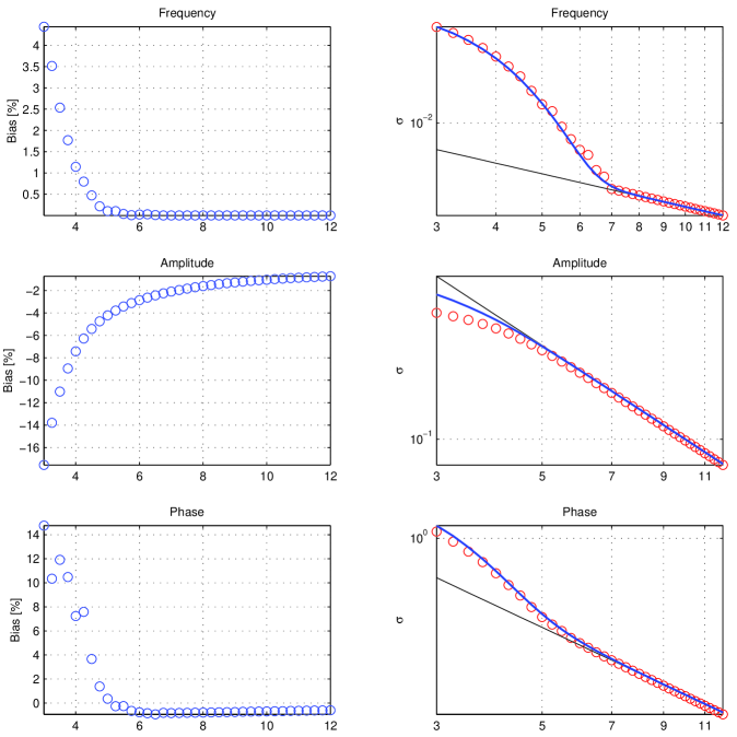
Figure 10: Simulations of the biases (plots on the left) and the rms errors (plots on the right) for a monochromatic signal. The results of the simulations are marked by the circles. The $x$-axes are labelled by the optimal signal-to-noise ratio. The thin solid lines in the plots on the right are calculated from the covariance matrix and the thick lines follow from Eqs. (137) and (140).

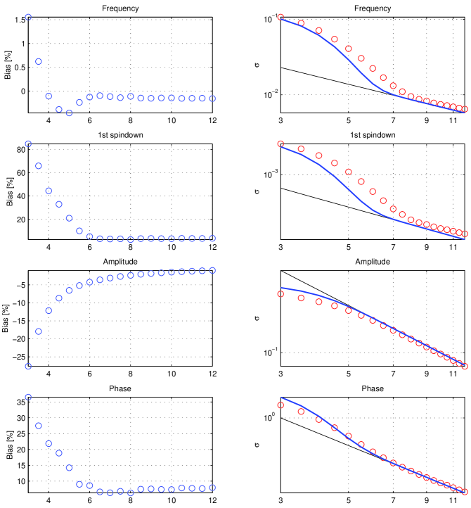
Figure 11: Simulations of the biases (plots on the left) and the rms errors (plots on the right) for a 1-spindown signal. The results of the simulations are marked by the circles. The $x$-axes are labelled by the optimal signal-to-noise ratio. The thin solid lines in the plots on the right are calculated from the covariance matrix and the thick lines follow from Eqs. (137) and (140).

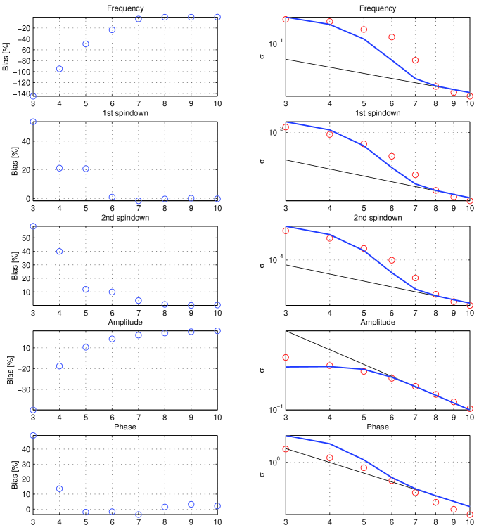
Figure 12: Simulations of the biases (plots on the left) and the rms errors (plots on the right) for a 2-spindown signal. The results of the simulations are marked by the circles. The $x$-axes are labelled by the optimal signal-to-noise ratio. The thin solid lines in the plots on the right are calculated from the covariance matrix and the thick lines follow from Eqs. (137) and (140).

In Figures 10, 11, and 12 we have presented the results of our simulations and we have compared them with the rms errors calculated from the covariance matrix. We have also calculated the errors from our simple model presented above using Eqs. (137) and (140). In the case of frequency, spindowns, and phase to calculate $\sigma_{out}$ we have assumed uniform probability density. The estimator of the amplitude is proportional to the modulus $|\widetilde{X}|$ of the Fourier transform of the data and in the case of the amplitude we have calculated $\sigma_{out}$ for the probability density of $|\widetilde{X}|$ assuming that there is no signal in the data. We see that the agreement between the simulated and calculated errors is very good. This confirms that our simple model is correct. We also give biases of the estimators in our simulations. We see from Figures 10–12 that as signal-to-noise ratio increases the simulated biases tend to zero and the standard deviations tend to rms errors calculated from the covariance matrices.

Appendix A Functions $A$, $B$, and $C$

The functions $A$, $B$, and $C$ in Eqs. (14) for the observation time chosen as an integer number of sidereal days take the form (here $n$ is a positive integer)

$$A\bigg{|}_{T_{o}=n\,2\pi/\Omega_{r}} = \frac{1}{16}\sin^{2}2\gamma\left[9\cos^{4}\lambda\cos^{4}\delta+\frac{1}{2}\sin^{2}2\lambda\sin^{2}2\delta+\frac{1}{32}\left(3-\cos 2\lambda\right)^{2}\left(3-\cos 2\delta\right)^{2}\right]$$ (141)

$$+\frac{1}{32}\cos^{2}2\gamma\left[4\cos^{2}\lambda\sin^{2}2\delta+\sin^{2}\lambda\left(3-\cos 2\delta\right)^{2}\right],$$

$$B\bigg{|}_{T_{o}=n\,2\pi/\Omega_{r}} = \frac{1}{32}\sin^{2}2\gamma\left[\left(3-\cos 2\lambda\right)^{2}\sin^{2}\delta+4\sin^{2}2\lambda\cos^{2}\delta\right]$$ (142)

$$+\frac{1}{4}\cos^{2}2\gamma\left(1+\cos 2\lambda\cos 2\delta\right),$$

$$C\bigg{|}_{T_{o}=n\,2\pi/\Omega_{r}} = 0.$$ (143)

We see that the functions $A$, $B$, and $C$ depend only on one unknown parameter of the signal—the declination $\delta$ of the gravitational-wave source. They also depend on the latitude $\lambda$ of the detector’s location and the orientation $\gamma$ of the detector’s arms with respect to local geographical directions.

Appendix B The Fisher matrix

In this appendix we give the explicit analytic formula for the Fisher matrix for the simplified model of the gravitational-wave signal from a spinning neutron star. The model is defined by Eqs. (55) and (56) in Sec. 4. It has a constant amplitude and its phase is linear in the parameters. In Paper II we have shown that this model reproduces well the accuracy of the estimators of the parameters calculated from the full model which has amplitude modulation and nonlinear phase. In this paper in Sec. 5 we show that the number of templates needed to perform all-sky searches calculated from the linear model reproduces well the number of templates calculated from the nonlinear phase model in Ref. [7]. Thus we see that the Fisher matrix presented below can be used in the theoretical studies of data analysis of gravitational-wave signals from spinning neutron stars instead of a very complex Fisher matrix for the full model.

In Paper II we have found that the Fisher matrix depends on the choice of the initial time within the observational interval (initial time is that instant of time at which the instantaneous frequency and the spindown parameters are defined, see Appendix C of Paper II). However one finds that the determinant of the transformation between the two Fisher matrices with different values of the initial time chosen is 1. Consequently the number of cells and the number of filters do not depend on the choice of initial time. We present our analytic formula for the initial time chosen to coincide with the middle of the observation interval. This simplifies the analytic expressions considerably.

The Fisher matrix $\Gamma_{(s)}^{\text{all}}$ for all-sky searches with $s$ spindowns included is defined by

$$\left(\Gamma_{(s)}^{\text{all}}\right)_{ij}:=\frac{1}{T_{o}}\int_{-T_{o}/2}^{T_{o}/2}\frac{\partial\Psi\left(t;\boldsymbol{\zeta}\right)}{\partial\zeta_{i}}\frac{\partial\Psi\left(t;\boldsymbol{\zeta}\right)}{\partial\zeta_{j}}dt,$$ (144)

where $\boldsymbol{\zeta}=(\Phi_{0},\boldsymbol{\xi})$, $\boldsymbol{\xi}=(\alpha_{1},\alpha_{2},\omega_{0},\ldots,\omega_{s})$, and the phase $\Psi$ is equal to

$$\Psi\left(t;\boldsymbol{\zeta}\right)=\Phi_{0}+\Phi\left(t;\boldsymbol{\xi}\right);$$ (145)

the function $\Phi$ is given by Eq. (56). We have calculated the Fisher matrix $\Gamma_{(s)}^{\text{all}}$ for $s=4$. The result is

$$\Gamma_{(4)}^{\text{all}}=\left(\begin{array}[]{cccccccc}1&\Gamma_{\Phi_{0}\alpha_{1}}&\Gamma_{\Phi_{0}\alpha_{2}}&0&\frac{1}{12}&0&\frac{1}{80}&0\\ &\Gamma_{\alpha_{1}\alpha_{1}}&\Gamma_{\alpha_{1}\alpha_{2}}&\Gamma_{\alpha_{1}\omega_{0}}&\Gamma_{\alpha_{1}\omega_{1}}&\Gamma_{\alpha_{1}\omega_{2}}&\Gamma_{\alpha_{1}\omega_{3}}&\Gamma_{\alpha_{1}\omega_{4}}\\ &&\Gamma_{\alpha_{2}\alpha_{2}}&\Gamma_{\alpha_{2}\omega_{0}}&\Gamma_{\alpha_{2}\omega_{1}}&\Gamma_{\alpha_{2}\omega_{2}}&\Gamma_{\alpha_{2}\omega_{3}}&\Gamma_{\alpha_{2}\omega_{4}}\\ &&&\frac{1}{12}&0&\frac{1}{80}&0&\frac{1}{448}\\ &&&&\frac{1}{80}&0&\frac{1}{448}&0\\ &&&&&\frac{1}{448}&0&\frac{1}{2304}\\ &&&&&&\frac{1}{2304}&0\\ &&&&&&&\frac{1}{11264}\end{array}\right),$$ (146)

where (here $\Xi_{o}:=\Omega_{o}T_{o}$ and $\Xi_{r}:=\Omega_{r}T_{o}$)

$$\Gamma_{\Phi_{0}\alpha_{1}} = \frac{4\pi r_{ES}}{c\Xi_{o}}\sin\phi_{o}\sin\frac{\Xi_{o}}{2}+\frac{4\pi r_{E}}{c\Xi_{r}}\cos\varepsilon\,\cos\lambda\,\sin\phi_{r}\sin\frac{\Xi_{r}}{2},$$

$$\Gamma_{\Phi_{0}\alpha_{2}} = \frac{4\pi r_{ES}}{c\Xi_{o}}\cos\phi_{o}\sin\frac{\Xi_{o}}{2}+\frac{4\pi r_{E}}{c\Xi_{r}}\cos\lambda\,\cos\phi_{r}\sin\frac{\Xi_{r}}{2},$$

$$\Gamma_{\alpha_{1}\alpha_{1}} = \frac{2\pi^{2}r_{ES}^{2}}{c^{2}}\left(1-\cos 2\phi_{o}\frac{\sin\Xi_{o}}{\Xi_{o}}\right)+\frac{2\pi^{2}r_{E}^{2}}{c^{2}}\cos^{2}\varepsilon\,\cos^{2}\lambda\left(1-\cos 2\phi_{r}\frac{\sin\Xi_{r}}{\Xi_{r}}\right)$$

$$+\frac{8\pi^{2}r_{E}r_{ES}}{c^{2}}\cos\varepsilon\,\cos\lambda\left[\cos(\phi_{o}-\phi_{r})\frac{\sin\frac{1}{2}(\Xi_{r}-\Xi_{o})}{\Xi_{r}-\Xi_{o}}-\cos(\phi_{o}+\phi_{r})\frac{\sin\frac{1}{2}(\Xi_{r}+\Xi_{o})}{\Xi_{r}+\Xi_{o}}\right],$$

$$\Gamma_{\alpha_{1}\alpha_{2}} = \frac{2\pi^{2}r_{ES}^{2}}{c^{2}}\sin 2\phi_{o}\frac{\sin\Xi_{o}}{\Xi_{o}}+\frac{2\pi^{2}r_{E}^{2}}{c^{2}}\cos\varepsilon\,\cos^{2}\lambda\,\sin 2\phi_{r}\frac{\sin\Xi_{r}}{\Xi_{r}}+\frac{8\pi^{2}r_{E}r_{ES}}{c^{2}\left(\Xi_{r}^{2}-\Xi_{o}^{2}\right)}\cos\lambda$$

$$\times\left\{\left[\cos\phi_{r}\sin\phi_{o}\left(\Xi_{r}\cos\varepsilon-\Xi_{o}\right)+\cos\phi_{o}\sin\phi_{r}\left(\Xi_{r}-\Xi_{o}\cos\varepsilon\right)\right]\cos\frac{\Xi_{r}}{2}\sin\frac{\Xi_{o}}{2}\right.$$

$$\left.+\left[\cos\phi_{r}\,\sin\phi_{o}\left(\Xi_{r}-\Xi_{o}\cos\varepsilon\right)+\cos\phi_{o}\,\sin\phi_{r}\left(\Xi_{r}\cos\varepsilon-\Xi_{o}\right)\right]\sin\frac{\Xi_{r}}{2}\cos\frac{\Xi_{o}}{2}\right\},$$

$$\Gamma_{\alpha_{1}\omega_{0}} = \frac{2\pi r_{ES}}{c\Xi_{o}^{2}}\cos\phi_{o}\left(2\sin\frac{\Xi_{o}}{2}-\Xi_{o}\cos\frac{\Xi_{o}}{2}\right)$$

$$+\frac{2\pi r_{E}}{c\Xi_{r}^{2}}\cos\varepsilon\,\cos\lambda\,\cos\phi_{r}\left(2\sin\frac{\Xi_{r}}{2}-\Xi_{r}\cos\frac{\Xi_{r}}{2}\right),$$

$$\Gamma_{\alpha_{1}\omega_{1}} = \frac{\pi r_{ES}}{c\Xi_{o}^{3}}\sin\phi_{o}\left[4\Xi_{o}\cos\frac{\Xi_{o}}{2}-\left(8-\Xi_{o}^{2}\right)\sin\frac{\Xi_{o}}{2}\right]$$

$$+\frac{\pi r_{E}}{c\Xi_{r}^{3}}\cos\varepsilon\,\cos\lambda\,\sin\phi_{r}\left[4\Xi_{r}\cos\frac{\Xi_{r}}{2}-\left(8-\Xi_{r}^{2}\right)\sin\frac{\Xi_{r}}{2}\right],$$

$$\Gamma_{\alpha_{1}\omega_{2}} = \frac{\pi r_{ES}}{2c\Xi_{o}^{4}}\cos\phi_{o}\left[\Xi_{o}\left(24-\Xi_{o}^{2}\right)\cos\frac{\Xi_{o}}{2}-6\left(8-\Xi_{o}^{2}\right)\sin\frac{\Xi_{o}}{2}\right]$$

$$+\frac{\pi r_{E}}{2c\Xi_{r}^{4}}\cos\varepsilon\,\cos\lambda\,\cos\phi_{r}\left[\Xi_{r}\left(24-\Xi_{r}^{2}\right)\cos\frac{\Xi_{r}}{2}-6\left(8-\Xi_{r}^{2}\right)\sin\frac{\Xi_{r}}{2}\right],$$

$$\Gamma_{\alpha_{1}\omega_{3}} = \frac{\pi r_{ES}}{4c\Xi_{o}^{5}}\sin\phi_{o}\left[8\Xi_{o}\left(-24+\Xi_{o}^{2}\right)\cos\frac{\Xi_{o}}{2}+\left(384-48\Xi_{o}^{2}+\Xi_{o}^{4}\right)\sin\frac{\Xi_{o}}{2}\right]$$

$$+\frac{\pi r_{E}}{4c\Xi_{r}^{5}}\cos\varepsilon\,\cos\lambda\,\sin\phi_{r}\left[8\Xi_{r}\left(-24+\Xi_{r}^{2}\right)\cos\frac{\Xi_{r}}{2}+\left(384-48\Xi_{r}^{2}+\Xi_{r}^{4}\right)\sin\frac{\Xi_{r}}{2}\right],$$

$$\Gamma_{\alpha_{1}\omega_{4}} = -\frac{\pi}{8c}\left\{\frac{r_{ES}}{\Xi_{o}^{6}}\cos\phi_{o}\left[\Xi_{o}\left(1920-80\Xi_{o}^{2}+\Xi_{o}^{4}\right)\cos\frac{\Xi_{o}}{2}-10\left(384-48\Xi_{o}^{2}+\Xi_{o}^{4}\right)\sin\frac{\Xi_{o}}{2}\right]\right.$$

$$\left.+\frac{r_{E}}{\Xi_{r}^{6}}\cos\varepsilon\,\cos\lambda\,\cos\phi_{r}\left[\Xi_{r}\left(1920-80\Xi_{r}^{2}+\Xi_{r}^{4}\right)\cos\frac{\Xi_{r}}{2}-10\left(384-48\Xi_{r}^{2}+\Xi_{r}^{4}\right)\sin\frac{\Xi_{r}}{2}\right]\right\},$$

$$\Gamma_{\alpha_{2}\alpha_{2}} = \frac{2\pi^{2}r_{ES}^{2}}{c^{2}}\left(1+\cos 2\phi_{o}\frac{\sin\Xi_{o}}{\Xi_{o}}\right)+\frac{2\pi^{2}r_{E}^{2}}{c^{2}}\cos^{2}\lambda\left(1+\cos 2\phi_{r}\frac{\sin\Xi_{r}}{\Xi_{r}}\right)$$

$$+\frac{8\pi^{2}r_{E}r_{ES}}{c^{2}}\cos\lambda\left[\cos(\phi_{o}-\phi_{r})\frac{\sin\frac{1}{2}(\Xi_{r}-\Xi_{o})}{\Xi_{r}-\Xi_{o}}+\cos(\phi_{o}+\phi_{r})\frac{\sin\frac{1}{2}(\Xi_{r}+\Xi_{o})}{\Xi_{r}+\Xi_{o}}\right],$$

$$\Gamma_{\alpha_{2}\omega_{0}} = \frac{2\pi r_{ES}}{c\Xi_{o}^{2}}\sin\phi_{o}\left(\Xi_{o}\cos\frac{\Xi_{o}}{2}-2\sin\frac{\Xi_{o}}{2}\right)+\frac{2\pi r_{E}}{c\Xi_{r}^{2}}\cos\lambda\,\sin\phi_{r}\left(\Xi_{r}\cos\frac{\Xi_{r}}{2}-2\sin\frac{\Xi_{r}}{2}\right),$$

$$\Gamma_{\alpha_{2}\omega_{1}} = \frac{\pi r_{ES}}{c\Xi_{o}^{3}}\cos\phi_{o}\left[4\Xi_{o}\cos\frac{\Xi_{o}}{2}-\left(8-\Xi_{o}^{2}\right)\sin\frac{\Xi_{o}}{2}\right]$$

$$+\frac{\pi r_{E}}{c\Xi_{r}^{3}}\cos\lambda\,\cos\phi_{r}\left[4\Xi_{r}\cos\frac{\Xi_{r}}{2}-\left(8-\Xi_{r}^{2}\right)\sin\frac{\Xi_{r}}{2}\right],$$

$$\Gamma_{\alpha_{2}\omega_{2}} = \frac{\pi r_{ES}}{2c\Xi_{o}^{4}}\sin\phi_{o}\left[-\Xi_{o}\left(24-\Xi_{o}^{2}\right)\cos\frac{\Xi_{o}}{2}+6\left(8-\Xi_{o}^{2}\right)\sin\frac{\Xi_{o}}{2}\right]$$

$$+\frac{\pi r_{E}}{2c\Xi_{r}^{4}}\cos\lambda\,\sin\phi_{r}\left[-\Xi_{r}\left(24-\Xi_{r}^{2}\right)\cos\frac{\Xi_{r}}{2}+6\left(8-\Xi_{r}^{2}\right)\sin\frac{\Xi_{r}}{2}\right],$$

$$\Gamma_{\alpha_{2}\omega_{3}} = \frac{\pi r_{ES}}{4c\Xi_{o}^{5}}\cos\phi_{o}\left[8\Xi_{o}\left(-24+\Xi_{o}^{2}\right)\cos\frac{\Xi_{o}}{2}+\left(384-48\Xi_{o}^{2}+\Xi_{o}^{4}\right)\sin\frac{\Xi_{o}}{2}\right]$$

$$+\frac{\pi r_{E}}{4c\Xi_{r}^{5}}\cos\lambda\,\cos\phi_{r}\left[8\Xi_{r}\left(-24+\Xi_{r}^{2}\right)\cos\frac{\Xi_{r}}{2}+\left(384-48\Xi_{r}^{2}+\Xi_{r}^{4}\right)\sin\frac{\Xi_{r}}{2}\right],$$

$$\Gamma_{\alpha_{2}\omega_{4}} = \frac{\pi}{8c}\left\{\frac{r_{ES}}{\Xi_{o}^{6}}\sin\phi_{o}\left[\Xi_{o}\left(1920-80\Xi_{o}^{2}+\Xi_{o}^{4}\right)\cos\frac{\Xi_{o}}{2}-10\left(384-48\Xi_{o}^{2}+\Xi_{o}^{4}\right)\sin\frac{\Xi_{o}}{2}\right]\right.$$

$$\left.+\frac{r_{E}}{\Xi_{r}^{6}}\cos\lambda\,\sin\phi_{r}\left[\Xi_{r}\left(1920-80\Xi_{r}^{2}+\Xi_{r}^{4}\right)\cos\frac{\Xi_{r}}{2}-10\left(384-48\Xi_{r}^{2}+\Xi_{r}^{4}\right)\sin\frac{\Xi_{r}}{2}\right]\right\}.$$

The above formulae could further be simplified if we assume that the observation time is an integer multiple of one sidereal day. We also note that if we have data corresponding to a full year we can start our observation at a time corresponding to any position of the detector in its motion around the Sun. This means that in such a case we can choose the phases $\phi_{r}$ and $\phi_{o}$ arbitrarily.

The Fisher matrix $\Gamma_{(s)}^{\text{all}}$ for $s=0,\ldots,3$ equals to the submatrix of $\Gamma_{(4)}^{\text{all}}$ consisting of the first $s+3$ columns and the first $s+3$ rows of $\Gamma_{(4)}^{\text{all}}$. The reduced matrix $\widetilde{\Gamma}_{(s)}^{\text{all}}$ defined in Eq. (73) can also be obtained from the matrix $\Gamma_{(s)}^{\text{all}}$ by means of the following procedure: take the inverse of $\Gamma_{(s)}^{\text{all}}$, remove the first column and the first row of the inverse, take again the inverse of such a submatrix—it equals $\widetilde{\Gamma}_{(s)}^{\text{all}}$.

In the case of directed searches the Fisher matrix $\Gamma_{(s)}^{\text{dir}}$ is also defined by Eq. (144), but now $\boldsymbol{\zeta}=(\Phi_{0},\boldsymbol{\xi})$, $\boldsymbol{\xi}=(\omega_{0},\ldots,\omega_{s})$, and the phase $\Phi$ is given by Eq. (82). The Fisher matrix $\Gamma_{(4)}^{\text{dir}}$ with $s=4$ spindowns included reads

$$\Gamma_{(4)}^{\text{dir}}=\left(\begin{array}[]{cccccccc}1&0&\frac{1}{12}&0&\frac{1}{80}&0\\ &\frac{1}{12}&0&\frac{1}{80}&0&\frac{1}{448}\\ &&\frac{1}{80}&0&\frac{1}{448}&0\\ &&&\frac{1}{448}&0&\frac{1}{2304}\\ &&&&\frac{1}{2304}&0\\ &&&&&\frac{1}{11264}\end{array}\right).$$ (147)

The Fisher matrix $\Gamma_{(s)}^{\text{dir}}$ for $s=0,\ldots,3$ equals to the submatrix of $\Gamma_{(4)}^{\text{dir}}$ consisting of $s+1$ first columns and $s+1$ first rows of $\Gamma_{(4)}^{\text{dir}}$. The reduced matrix $\widetilde{\Gamma}_{(s)}^{\text{dir}}$ defined by Eq. (73) can be obtained from the matrix $\Gamma_{(s)}^{\text{dir}}$ by means of the same procedure as described above for the case of all-sky searches.

Appendix C Suboptimal filtering

Very often suboptimal filter (or a search template) is proposed in hierarchical signal searches. In such a search one passes the data through a suboptimal filter that requires much less computational cost than the optimal filter and one registers the condidate events. Then one passes the data through optimal filters however only for the values (or around the values) of the parameters of the candidate events to assess the significance of the candidate events. In such a search one would like to ensure that there is no loss of events. A way to achieve this when using a suboptimal filter is to lower the threshold with respect to the threshold chosen for the optimal filter so that the number of expected significant events is the same as with the optimum filter. The probability densities derived in Sec. 6.1 can be used to calculate what the lowered threshold should be.

To illustrate the general theory developed in Sec. 6 we have considered the following example. We have assumed the observation time $T_{o}$ to be 3 days and we have restricted ourselves to directed searches. For such a case the model of the phase consistent with the 1/4 of a cycle criterion has $s_{1}=2$ spindowns in the dominant term, $s_{2}=1$ spindown in the contribution due to the Earth orbital motion and no contribution due to the Earth diurnal motion ($s_{3}=0$), cf. Eq. (134). We have correlated this signal with a template that has $s_{1}=1$, $s_{2}=1$, and $s_{3}=0$. Assuming the gravitational-wave frequency $f_{o}=1$ kHz and the maximum values of the spindowns for the spindown age $\tau=40$ yr the fitting factor is 0.91, the number of cells $N_{c}$ for the optimal random field is $2.3\times 10^{12}$ and the number of cells $N_{sc}$ for the suboptimal random field is $3.7\times 10^{12}$. We have found that the fitting factor is practically independent on the right ascension and the declination of the gravitational-wave source.

In our computations we assume that we lower the threshold according to the law

$${\mathcal{F}}_{oL}=({\mathcal{F}}_{o}-1)\text{FF}^{2}+1.$$ (148)

The above rule is motivated by the relation between the expectation value of the statistics ${\mathcal{F}}$ and the optimal signal-to-noise ratio given by Eq. (89).

The numerical results obtained using formulae derived in Sec. 6.1 are presented in Figure 13. We have assumed the false alarm probability to be 1% for the optimal filter. There is one more input parameter that we need in order to calculate the numbers of expected events: the signal-to-noise ratio $d_{1}$ for which the number of events is 1. In the upper left plot in Figure 13 we have shown the ratio of the expected number of the detected events for the suboptimal filtering [calculated from Eq. (119)] and the optimal one [calculated from Eq. (118)] as a function of $d_{1}$. We have assumed that in the suboptimal filter we lower the threshold according to Eq. (148). We have also put $\text{FF}=0.91$.

To assess the number of events that one loses using a search template Apostolatos [22] assumed that the number of detected events decreases as FF³. In the right upper plot of Figure 13 we have compared the number of detected events calculated from Eq. (119) and the ones calculated using FF³ law. We see that in general FF³ law underestimates the event loss. However for the fitting factors close to one the difference is small.

We have calculated the numbers of expected detections and false alarms for the optimal and suboptimal filter both with original and lowered thresholds. The results are presented in the two lower plots in Figure 13. In the plot on the left diamonds mark the ratio of the number of the detected events for the suboptimal filter with lowered threshold [calculated from Eqs. (119) and (148)] and the number of events detected with the optimum filter [calculated from Eq. (118)]; squares denote the ratio of the number of events detected by suboptimal filtering without lowering the threshold and the number of events detected with the optimum filter; the solid line gives the fraction of the detected events calculated from FF³ law; all dependencies are shown as functions of the fitting factor. The lower plot on the right gives the ratio of the expected number of false alarms with the suboptimal filter and lowered threshold and the expected number of false alarms for the optimal filter.

From our example we see that when using a suboptimal filter by appropriate lowering of the threshold we can detect all that events that can be detected with an optimal filter. There is however a limitation to threshold lowering arising from the fact that below a certain threshold the false alarm rate can increase to an unmanageable level. In the real data analysis there may be other limitations. For example below a certain threshold a forest of non-Gaussian events may appear completely obscuring the real signals.

Appendix D The use of parameters $\alpha_{1}$ and $\alpha_{2}$ to label the filters

If one knows the values of the parameters $\alpha_{1}$, $\alpha_{2}$, and $f_{o}$ it is possible to solve Eqs. (58) with respect to the angles $\alpha$ and $\delta$. One can show that each triple $(\alpha_{1},\alpha_{2},f_{o})$ gives two such solutions which can be written as follows (note that because $\delta\in[-\frac{\pi}{2},\frac{\pi}{2}]$ to determine $\delta$ uniquely it is enough to know $\sin\delta$):

$$\sin\delta = \beta_{1}\sin\varepsilon\pm\sqrt{1-\beta_{1}^{2}-\beta_{2}^{2}},$$ (149)

$$\cos\delta = \sqrt{1-\sin^{2}\delta},$$ (150)

$$\sin\alpha = \frac{\beta_{1}-\sin\varepsilon\sin\delta}{\cos\varepsilon\cos\delta},$$ (151)

$$\cos\alpha = \frac{\beta_{2}}{\cos\delta},$$ (152)

where

$$\beta_{1}:=\frac{\alpha_{1}}{f_{o}},\quad\beta_{2}:=\frac{\alpha_{2}}{f_{o}}.$$ (153)

The correspondence between the parameters $\alpha_{1}$, $\alpha_{2}$, $f_{o}$ and $\alpha$, $\delta$ given by Eqs. (149)–(152) implies that one can use $\alpha_{1}$, $\alpha_{2}$ instead of $\alpha$, $\delta$ to label the templates needed for matched filtering. To do this the family of templates labelled by $\alpha$, $\delta$ (and the other parameters) must be replaced by two template families labelled by $\alpha_{1}$, $\alpha_{2}$ (and the other parameters). The first family arises when in the original family one replaces $\sin\delta$, $\cos\delta$, $\sin\alpha$, and $\cos\alpha$ by the left-hand sides of Eqs. (149)–(152) with $+$ sign chosen in the front of the square root in Eq. (149). In the second family the replacements are made with $-$ sign chosen. The filters labelled by parameters $\alpha_{1}$ and $\alpha_{2}$ will to a good appproximation be linear and the theory of data processing developed in this paper applies to such a filtering scheme.

When as a result of filtering of the data one gets a significant event one obtains at the same time the maximum likelihood estimators of the parameters $\alpha_{1}$, $\alpha_{2}$, $f_{o}$ (and the others). One can obtain the maximum likelihood estimators of the position $(\alpha,\delta)$ of the gravitational-wave source in the sky by means of Eqs. (149)–(152). Note that one should expect to get the maximum correlation for a template belonging to one out of two families described above, what means that after filtering one would also know which sign on the left-hand side of Eq. (149) should be chosen.

The covariance matrix for the parameters $\alpha$, $\delta$, and $f_{o}$ can be obtained from the covariance matrix for the parameters $\alpha_{1}$, $\alpha_{2}$, and $f_{o}$ by means of the law of propagation of errors. Let us introduce

$${\mathbf{x}}:=(\alpha_{1},\alpha_{2},f_{o}),\quad{\mathbf{y}}:=(\alpha,\delta,f_{o}).$$ (154)

Let $C_{\mathbf{x}}$ be the covariance matrix for the parameters ${\mathbf{x}}$, then the covariance matrix $C_{\mathbf{y}}$ for the parameters ${\mathbf{y}}$ can be calculated as follows:

$$C_{\mathbf{y}}=JC_{\mathbf{x}}J^{T},$$ (155)

where $T$ denotes matrix transposition and the Jacobi matrix $J$ has components:

$$J=\left(\begin{array}[]{ccc}{\displaystyle\frac{\partial\alpha}{\partial\alpha_{1}}}&{\displaystyle\frac{\partial\alpha}{\partial\alpha_{2}}}&{\displaystyle\frac{\partial\alpha}{\partial f_{o}}}\\[8.61108pt] {\displaystyle\frac{\partial\delta}{\partial\alpha_{1}}}&{\displaystyle\frac{\partial\delta}{\partial\alpha_{2}}}&{\displaystyle\frac{\partial\delta}{\partial f_{o}}}\\[8.61108pt] 0&0&1\end{array}\right).$$ (156)

All derivatives entering Eq. (156) can be calulated using Eqs. (149)–(152).

Figure 4: Volume of one cell (in units s^-2) in all-sky searches as a function of the observation time $T_{o}$ for the LIGO Hanford detector (latitude $\lambda=46.45^{\circ}$). We have calculated the volume of one cell from Eq. (79). The lines shown in the plot correspond to different numbers $s$ of spindowns included: $s=4$ (solid), $s=3$ (dotted), $s=2$ (dashed), $s=1$ (dotted/dashed), and $s=0$ (double dotted/dashed). We have set $\phi_{r}=1.456$ and $\phi_{o}=0.123$.

Figure 13: Suboptimal filtering. In the upper left plot we show the ratio $N_{sD}(d_{1\text{sub}},{\mathcal{F}}_{oL})/N_{D}(d_{1},{\mathcal{F}}_{o})$ of the expected number of the detected events for the suboptimal filtering [calculated from Eq. (119)] and the optimal one [calculated from Eq. (118)] as a function of the signal-to-noise ratio $d_{1}$ (the signal-to-noise ratio for which the number of events is one). We have assumed that in the suboptimal filter we lower the threshold according to Eq. (148). We have also put $\text{FF}=0.91$. In the right upper plot we give the ratio $r=[N_{sD}(d_{1\text{sub}},{\mathcal{F}}_{oL})/N_{D}(d_{1},{\mathcal{F}}_{o})]/\text{FF}^{3}$ as a function of the fitting factor (we have used $d_{1}=16.6$). In the left lower plot diamonds mark the ratio $N_{sD}(d_{1\text{sub}},{\mathcal{F}}_{oL})/N_{D}(d_{1},{\mathcal{F}}_{o})$ of the number of the detected events for the suboptimal filter with lowered threshold [calculated from Eqs. (119) and (148)] and the number of events detected with the optimum filter [calculated from Eq. (118)]; squares denote the ratio $N_{sD}(d_{1\text{sub}},{\mathcal{F}}_{o})/N_{D}(d_{1},{\mathcal{F}}_{o})$ of the number of events detected by suboptimal filtering without lowering the threshold and the number of events detected with the optimum filter; the solid line gives the fraction of the detected events calculated from FF³ law; all dependencies are shown as functions of the fitting factor (we have put $d_{1}=16.6$). The lower plot on the right gives the ratio of the expected number of false alarms with the suboptimal filter and lowered threshold and the expected number of false alarms for the optimal filter.

References

- [1] K. Danzmann et al., in Gravitational Wave Experiments, edited by E. Coccia, G. Pizzella, and F. Ronga (World Scientific, Singapore, 1995), pp. 100–111.
- [2] A. Abramovici et al., Science 256, 325 (1992).
- [3] C. Bradaschia et al., Nucl. Instrum. Methods Phys. Res. A 289, 518 (1990).
- [4] K. Tsubono et al., in Gravitational Wave Detection. Proceedings of the TAMA International Workshop on Gravitational Wave Detection, edited by K. Tsubono, M.-K. Fujimoto, and K. Kuroda (Universal Academy Press, Tokyo, 1997), pp. 183–191.
- [5] P. Jaranowski, A. Królak, and B. F. Schutz, Phys. Rev. D 58, 063001 (1998).
- [6] P. Jaranowski and A. Królak, Phys. Rev. D, in press, gr-qc/9809046.
- [7] P. R. Brady, T. Creighton, C. Cutler, and B. F. Schutz, Phys. Rev. D 57, 2101 (1998).
- [8] N. Andersson, Astrophys. J., in press, gr-qc/9706075.
- [9] L. Lindblom, B. J. Owen, and S. M. Morsink, Phys. Rev. Lett. 80, 4843 (1998).
- [10] B. J. Owen, L. Lindblom, C. Cutler, B. F. Schutz, A. Vecchio, and N. Andersson, Phys. Rev. D 58, 084020 (1998).
- [11] L. Bildsten, Astrophys. J., in press, astro-ph/9804325.
- [12] M. H. A. Davis, in Gravitational Wave Data Analysis, edited by B. F. Schutz (Kluwer, Dordrecht, 1989), pp. 73–94.
- [13] R. Adler, The Geometry of Random Fields (John Wiley & Sons, 1981).
- [14] C. W. Helström, Statistical Theory of Signal Detection, 2nd ed. (Pergamon Press, London, 1968).
- [15] H. Cramér and M. R. Leadbetter, Stationary and Related Stochastic Processes (Sample Function Properties and Their Applications) (John Wiley & Sons, 1967).
- [16] K. J. Worsley, Advances in Applied Probability 26, 13 (1994).
- [17] D. B. Percival and A. T. Walden, Spectral Analysis for Physical Applications (Cambridge University Press, Cambridge, 1993), p. 222.
- [18] Formula (61) is derived in L. S. Finn, Phys. Rev. D 46, 5236 (1992), and formula (62) was obtained by us; in the proof of (62) we have used Lemma 5.3.1 from Ref. [13], p. 108.
- [19] B. J. Owen, Phys. Rev. D 53, 6749 (1996).
- [20] A. Królak, in Proceedings of the Cornelius Lanczos International Conference, edited by J. D. Brown, M. T. Chu, D. C. Ellison, and R. J. Plemmons (SIAM, Philadelphia, 1994), p. 482.
- [21] A. Królak, K. D. Kokkotas, and G. Schäfer, Phys. Rev. D 52, 2089 (1995).
- [22] T. A. Apostolatos, Phys. Rev. D 52, 605 (1995).
- [23] P. Astone et al., Phys. Rev. D 47, 362 (1993).
- [24] H. L. Van Trees, Detection, Estimation and Modulation Theory, Part I (Wiley, New York, 1969).
- [25] K. D. Kokkotas, A. Królak, and G. Tsegas, Class. Quantum Grav. 11, 1901 (1994).
- [26] R. Balasubramanian, B. S. Sathyaprakash, and S. V. Dhurandhar, Phys. Rev. D 53, 3033 (1996).
- [27] D. Nicholson and A. Vecchio, Phys. Rev. D 57, 4588 (1998).
- [28] D. C. Rife and R. R. Boorstyn, IEEE Transactions on Information Theory IT-20, 591 (1974).