Relativistic dust disks and the Wilson-Mathews approach

Abstract

Treating problems in full general relativity is highly complex and frequently approximate methods are employed to simplify the solution. We present comparative solutions of a infinitesimally thin relativistic, stationary, rigidly rotating disk obtained using the full equations and the approximate approach suggested by Wilson & Mathews. We find that the Wilson-Mathews method has about the same accuracy as the first post-Newtonian approximation.

I Introduction

The numerical solution of Einstein’s field equations in three spatial dimensions in simulating for example the merging process of two neutron stars is very complicated, and only very recently have methods been developed for treating such problems in full general relativity. One of the main difficulties is encountered in the treatment of the radiation degrees of freedom. An approximation scheme developed by Wilson & Mathews [1] simplifies the problem by imposing a conformally flat condition on the three metric, throwing away all radiation degrees of freedom. This reduces firstly the number of field equations and secondly reduces them to Poisson like equations exclusively. In general, the first post-Newtonian approximation of Einstein’s theory is identical to the one of the Wilson-Mathews scheme, and in spherical symmetry Wilson-Mathews is identical with Einstein.

As pointed out by Cook et al. [2], this approximation should be viable and verifiable for systems in a true equilibrium state. They investigated the accuracy of Wilson & Mathews’ approximative scheme on isolated rapidly rotating relativistic stars, and found largest errors of about 5% for any quantity analyzed. As the approximate scheme has been used in calculating the evolution of a binary system [3] which is very far from spherical symmetry, it is desirable to have test cases, that depart stronger from spherical symmetry than rotating stars do.

Here we present the model of an infinitesimally thin, pressureless disk that rotates rigidly. This problem was considered by Bardeen & Wagoner [4] up to the tenth post-Newtonian approximation and has been solved exactly by Neugebauer & Meinel [5]. Thus, it serves as an ideal test bed to check the validity of any numerical method solving the stationary, axisymmetric field equations [6] and in particular Wilson & Mathews’ approximation scheme. To demonstrate the general accuracy of the numerical method employed we present the numerical solution of the full Einstein equations as well.

II Basic Equations

To describe the stationary, axisymmetric equilibrium of an infinitesimally thin disk we use a cylindrical coordinate system ($c=1$, $c$ velocity of light)

$$x_{0}=t,x_{1}=\rho,x_{2}=z,x_{3}=\varphi$$ (1)

where the disk is located in the equatorial plane (z=0), and the rotation axis coincides with the $z$-axis.

A Full Einstein equations

The general line element for an axisymmetric and stationary mass configuration can be written as [4]

$$ds^{2}=e^{2\mu}\left(d\rho^{2}+dz^{2}\right)+[\rho Be^{-\nu}(d\varphi-\omega dt)]^{2}-e^{2\nu}dt^{2},$$ (2)

where the metric potentials $\nu,\mu,\omega$ and $B$ are functions of $\rho$ and $z$. As the disk has no vertical extension, the global solution of the problem may be obtained by solving the vacuum field equations, where the presence of the disk manifests itself through jump conditions in the first (vertical) $z-$derivatives of the metric functions.

As shown by [4] and [6], the vacuum Einstein equations $G_{ij}=0$ for the metric (2) are then given explicitly by

$$\nabla(\nabla\nu) = \frac{1}{2}\rho^{2}B^{2}e^{-4\nu}\nabla\omega\cdot\nabla\omega-\frac{1}{B}\nabla B\cdot\nabla\nu$$ (3)

$$\frac{1}{\rho^{2}}\nabla(\rho^{2}\nabla\omega) = -\frac{1}{a}\nabla a\cdot\nabla\omega,\hskip 11.38092pt\mbox{with}\hskip 7.11317pta:=\frac{B^{3}}{e^{4\nu}}$$ (4)

$$\nabla(\rho\nabla B) = 0$$ (5)

$$\Delta_{c}\mu = \frac{1}{4}\rho^{2}B^{2}e^{-4\nu}\nabla\omega\cdot\nabla\omega+\frac{1}{B}\nabla B\cdot\nabla\nu$$ (6)

$$- \nabla{\nu}\cdot\nabla\nu+\frac{1}{\rho}\frac{\partial\nu}{\partial\rho},$$ (7)

with the $\nabla$-Operator in cylindrical coordinates ($\rho,z$), and the Cartesian (in $\rho$ and $z$) Laplace operator $\Delta_{c}$.

The boundary conditions in the equatorial plane within the disk region $\rho<\rho_{d}$, where $\rho_{d}$ denotes the outer disk radius are then given by (see [6])

$$\nu_{,z} = 2\pi\sigma\,\frac{1+v_{\varphi}^{2}}{1-v_{\varphi}^{2}}$$ (8)

$$\omega_{,z} = -8\pi\sigma\,\frac{\Omega-\omega}{1-v_{\varphi}^{2}}$$ (9)

$$B_{,z} = 0$$ (10)

$$\mu_{,z} = -2\pi\sigma.$$ (11)

Here $\sigma$ and $P$ denote the surface density and pressure, and $v_{\varphi}=\rho Be^{-2\nu}(\Omega-\omega)$ is the orbital velocity of the gas. We note that in case of a pressureless ($P=0$) dust disk the metric function $B$ is identical to unity [4].

Radial hydrostatics yields the relation $e^{\nu}\left(1-v_{\varphi}^{2}\right)^{1/2}=const.$ in the disk, where $\rho\leq\rho_{d}$. In the outer part of the equatorial plane, $\rho>\rho_{d}$, and along the polar axis symmetry conditions are used for the metric coefficients. At infinity $\nu,\mu,$ and $\omega$ tend to zero, and $B=1$.

B Wilson-Mathews formulation

The method developed by Wilson and Mathews [1] consists in approximating the line element (2) by using a spatially isotropic form and neglecting the non-isotropic parts. Specifically, for the problem at hand we rewrite the exact metric as

$$ds^{2} = e^{2\tilde{\mu}}\left[\left(d\rho^{2}+dz^{2}\right)+\rho^{2}(d\varphi-\tilde{\omega}dt)^{2}\right]$$ (12)

$$+ \rho^{2}\tilde{B}^{2}(d\varphi-\tilde{\omega}dt)^{2}-e^{2\tilde{\nu}}dt^{2}$$ (13)

with the functions $\tilde{\nu}$, $\tilde{B}$, $\tilde{\mu}$ and $\tilde{\omega}$.

By comparison with (2) we may identify

$$e^{2\mu}=e^{2\tilde{\mu}},\omega=\tilde{\omega},\nu=\tilde{\nu}$$ (14)

and for the metric function $\tilde{B}$ we obtain

$$B^{2}=(e^{2\tilde{\mu}}+\tilde{B}^{2})e^{2\tilde{\nu}}.$$ (15)

Applying the approximation by Wilson & Mathews, we neglect the non-isotropic part and set $\tilde{B}=0$. Simultaneously we have to omit the corresponding field equation (for $B$), and we obtain the approximate field equations from (3), (4), and (7) by setting $B=e^{\tilde{\nu}+\tilde{\mu}}$

$$\nabla(\nabla\tilde{\nu}) = \frac{1}{2}\rho^{2}e^{2(\tilde{\mu}-\tilde{\nu})}\nabla\tilde{\omega}\cdot\nabla\tilde{\omega}-\nabla(\tilde{\nu}+\tilde{\mu})\cdot\nabla\tilde{\nu}$$ (16)

$$\nabla(\rho^{2}\nabla\tilde{\omega}) = -\rho^{2}\nabla(3\tilde{\mu}-\tilde{\nu})\cdot\nabla\tilde{\omega},$$ (17)

$$\Delta_{c}\tilde{\mu} = \frac{1}{4}\rho^{2}e^{2(\tilde{\mu}-\tilde{\nu})}\nabla\tilde{\omega}\cdot\nabla\tilde{\omega}+\nabla\tilde{\mu}\cdot\nabla\tilde{\nu}+\frac{1}{\rho}\frac{\partial\tilde{\nu}}{\partial\rho}$$ (18)

Furthermore, we have to substitute for $B$ in the equation for the orbital velocity, and obtain $v_{\varphi}=\rho e^{(\tilde{\mu}-\tilde{\nu})}(\Omega-\tilde{\omega})$. For our test case of a rigidly rotating dust disk ($B=1$) we may summarize the exact Einstein metric and the approximative Wilson-Mathews form as

$$ds^{2}=e^{2\mu}\left[\left(d\rho^{2}+dz^{2}\right)+\rho^{2}e^{-2(\nu+\mu)}(d\varphi-\omega dt)^{2}\right]\\ -e^{2\nu}dt^{2},$$ (19)

and

$$ds^{2}=e^{2\tilde{\mu}}\left[\left(d\rho^{2}+dz^{2}\right)+\rho^{2}(d\varphi-\tilde{\omega}dt)^{2}\right]\\ -e^{2\tilde{\nu}}dt^{2},$$ (20)

respectively. Comparing (19) and (20), it is striking that the only difference between exact and approximate method for the dust disk example lies in the function $e^{2\zeta}\equiv e^{2(\nu+\mu)}$. The function $\zeta$ gives the deviation from three-dimensional conformal flatness in Einstein’s theory and it has been shown that in the first post-Newtonian approximation $\zeta$ vanishes for the dust disk solution [4].

C Method of solution

The field equations for the exact and the approximate case together with the boundary conditions are solved numerically for the problem of a rigidly rotating dust disk. As the numerical procedure has been described in more detail by Kley [6] we give here only a brief sketch of the method. To prevent problems with the conditions at infinity the computational domain $[0:\infty;0:\infty]$ is mapped onto the unit square where the radius $\rho_{d}$ of the disk is located at $1/2$. This domain is covered here by $50\times 50$ gridcells and the partial differential equations are discretized to second order spatial accuracy on this grid yielding a coupled system of equations. Together with the boundary jump conditions these equations are then solved iteratively until convergence has been achieved. The accuracy of the solutions may be estimated using the analytical solution [5] and post-Newtonian approximation [4] of the dust disk.

III Results

To give an idea of the degree of non-isotropy of the three metric for the exact Einsteinian disk we display in Figure 1 the behaviour of the function $\zeta(\rho)$ within the disk for different values of the central redshift. In the figure the numerically obtained solution of the field equations (3)-(7) together with the boundary conditions (8)-(11) is compared to the exact solution as given by [5]. The errors over the whole disk for all central redshifts are usually well below 1% and only at the outer edge of the disk the worst deviation is about 2% for $z=3$. This demonstrates the accuracy of the numerical method employed, even for the moderate gridsize used.

FIG. 1.: The function $e^{2\zeta}$ which gives the deviation from local flatness plotted for the Einsteinian dust disk as function of the normalized radius $\rho/\rho_{d}$ for three different central redshifts of the disk. The diamonds refer to the numerical solution of the full Einstein equations, while the solid lines refer to the exact solution.

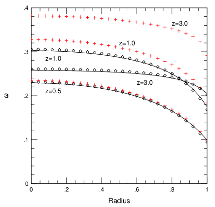
FIG. 2.: The metric function $\omega$ as a function of the normalized radius $\rho/\rho_{d}$ for three different central redshifts of the disk. The diamonds refer to the numerical solution of the full Einstein equations, while the crosses denote the numerical solution obtained by using the Wilson-Mathews approach. The solid lines refer to the exact solution.

We compared the numerically obtained approximate metric coefficients $\tilde{\nu}$, $\tilde{\mu}$ and $\tilde{\omega}$ versus radius with the exact solution and find that in case of the ”lapse” potential $\nu$ the deviation from the exact case is always below 2.5%, even for central redshifts as large as 3. For the function $\mu$ the deviation is larger, 2.3% for $z=0.5$, 5.5% for $z=1.0$, and about 20% for $z=3$. The results for the metric function $\omega$ are displayed in Fig. 2. The errors are very large for higher redshifts, about 9% for $z=1$ and up to 48% for $z=3$. The approximate solution (crosses) shows also the wrong trend of the evolution of $\omega$ with redshift. While in the Einsteinian disk case $\omega$ increases first with redshift, and then decreases for $z>2$, in the approximative solution $\omega$ seems to increase steadily with $z$.

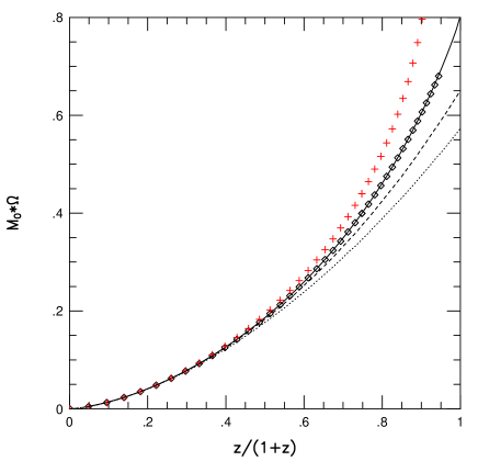
FIG. 3.: The quantity $\Omega M_{0}$ as a function of central redshift $z$ for the dust disk. The open squares correspond to the numerical solution of the full Einstein equations, the crosses to the approximate Wilson-Mathews procedure. The solid line refers to the exact solution, and the dotted and dashed line to the first and second post-Newtonian approximation respectively, of the Einstein equations.

The overall deviations of the metric functions from the exact case may be understood qualitatively by looking at the line elements (19) and (20). As the lapse is not too much affected by the simplification in the spatial three metric it will be calculated quite accurately in the Wilson-Mathews approach. The rotational coefficient $\omega$ is affected mostly and hence shows the largest errors. We may nevertheless infer that at least for central redshifts up to $z=0.5$ the approximate solution is very accurate, but for higher relativistic disks the agreement deteriorates. Note, that $z=.55$ was the maximum (polar) redshift tested in the comparison for rotating stars by Cook et al. [2].

As a further illustration of the range of applicability of the Wilson-Mathews approximation, it is interesting to plot global quantities. In Fig. 3 we display the dependence of the dimensionless quantity $\Omega M_{0}$ versus the parameter $\gamma=z/(1+z)$. One notices again the very good agreement of the numerical and exact solution of the full Einstein equations. Interestingly, the post-Newtonian approximations approach the exact solution from below while the Wilson-Mathews approximation lies always above the exact solution. In case of the full Einsteinian disk for infinite central redshift $\Omega*M_{0}$ reaches a finite maximum of about $0.8$.

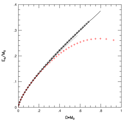
FIG. 4.: The binding energy as a function of $\Omega M_{0}$. The symbols are identical to Figure 3.

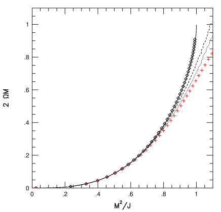
FIG. 5.: Dimensionless combination of the parameters measurable at infinity: gravitational mass $M$, angular momentum $J$ and angular velocity $\Omega$. The symbols are identical to Figure 3.

In Fig. 4 the normalized binding energy $E_{b}/M_{0}=1-M/M_{0}$ is plotted versus $\Omega M_{0}$. For a given rest mass $M_{0}$ and angular rotation rate $\Omega$ the Wilson-Mathews approximation yields a lower binding energy for the dust disk than the Einstein disk. The dotted line for the post-Newtonian solution ends at $\Omega*M_{0}=0.57$ because this refers already to $z=\infty$ (cf. Fig. 3).

Finally, in Figure 5 the dimensionless rotation rate $M\Omega$ is plotted versus the dimensionless total angular momentum $M^{2}/J$, parameters that are measurable at infinity. The value $2\Omega M=M^{2}/J=1$ corresponds to the extreme Kerr limit of the dust disk solution (see [5]). Again, the Wilson-Mathews approximation lies beyond the post-Newtonian approximation and does not yield the correct black hole limit.

IV Conclusions

We have calculated numerically model sequences of a rigidly rotating disk of dust using a) the full Einstein equations and b) the modified Wilson-Mathews scheme. By comparing those to the known exact solution by Neugebauer & Meinel [5], we have shown that the Wilson-Mathews approximation yields results which are accurate to about 5% if the central redshift of the disk is smaller than 0.5; but may be significantly higher for stronger relativistic models. We conclude that the Wilson-Mathews approach for solving the Einstein equations yields results which are at most as accurate as the first post-Newtonian approximation, at least for rigidly rotating disks of dust. Hence, its application to stronger relativistic configurations e.g. in close, compact binary systems has to be handled with caution.

REFERENCES

- [1] J.R. Wilson, G.J. Mathews, in Frontiers in Numerical Relativity, Eds. Evans et al. (1988, Urbana, Ill.); J.R. Wilson, G.J. Mathews, PRL 75, 4161 (1995); J.R. Wilson, G.J. Mathews and P. Marronetti, PRD 54, 1317 (1996).
- [2] G.B. Cook, S.L. Shapiro, and S.A. Teukolsky, PRD 53, 5533 (1996).
- [3] T. W. Baumgarte, G.B. Cook, M.A. Scheel, S.L. Shapiro, and S.A. Teukolsky, PRD 57, 7299 (1998).
- [4] J.M. Bardeen and R.V. Wagoner, Astrophys. J. 167, 359 (1971).
- [5] G. Neugebauer and R. Meinel, Astrophys. J. 414, L97 (1993); G. Neugebauer and R. Meinel, PRL 75, 3046 (1995).
- [6] W. Kley, Mon. Not. Roy. Astron. Soc. 287, 26 (1997).