Isolated Horizons:
A Generalization of Black Hole Mechanics

Abstract

A set of boundary conditions defining a non-rotating isolated horizon are given in Einstein-Maxwell theory. A space-time representing a black hole which itself is in equilibrium but whose exterior contains radiation admits such a horizon . Physically motivated, (quasi-)local definitions of the mass and surface gravity of an isolated horizon are introduced. Although these definitions do not refer to infinity, the quantities assume their standard values in Reissner-Nordström solutions. Finally, using these definitions, the zeroth and first laws of black hole mechanics are established for isolated horizons.

The similarity between the laws of black hole mechanics and those of ordinary thermodynamics is one of the most remarkable results to emerge from classical general relativity [1, 2, 3]. However, in the standard formulation, the zeroth and first laws apply only to stationary black holes. From a physical perspective, the requirement of stationarity seems too strong since it excludes situations in which there may be radiation far away from the black hole. Indeed, in a realistic gravitational collapse (depicted in figure 1a), although one expects the horizon to reach an equilibrium state at late times, one also expects gravitational and other radiation to be present near null infinity. One would hope that the familiar laws of black hole mechanics continue to hold in such situations. The purpose of this letter is to show that this expectation is correct: We will outline a new framework to describe a generic (non-rotating) isolated black hole and extend the laws of black hole mechanics to this broader class of space-times. This framework also serves as the point of departure for analyzing the quantum geometry of horizons non-perturbatively, which in turn provides a statistical mechanical explanation of the Bekenstein-Hawking entropy associated with the horizon [4].

The key idea is to replace the notion of a stationary black hole with that of an isolated horizon. This can be identified with a portion of the event horizon which is in equilibrium, i.e., across which there is no flux of gravitational radiation or matter fields. Examples of isolated horizons are shown in figures 1a and 1b. For technical simplicity, in this letter we will restrict our attention to non-rotating horizons.

\psfrag{Ifs}{\Large$\mathfs{I}^{+}$}\psfrag{Mcal}{\Large$\mathcal{M}$}\psfrag{i+}{\Large$i^{+}$}\psfrag{i0}{\Large$i^{0}$}\psfrag{Delta}{\Large$\Delta$}\psfrag{Mpln}{\Large$M$}\includegraphics{collapse.eps}

(a)

(b)

Figure 1: (a) A typical gravitational collapse. The portion $\Delta$ of the horizon at late times is isolated. The space-time $\mathcal{M}$ of interest is the triangular region bounded by $\Delta$, $\mathfs{I}^{+}$ and a partial Cauchy slice $M$.  (b) Space-time diagram of a black hole which is initially in equilibrium, absorbs a small amount of radiation, and again settles down to equilibrium. Portions $\Delta_{1}$ and $\Delta_{2}$ of the horizon are isolated.

Initially, the difference between static black holes and non-rotating isolated horizons may appear rather small. Therefore, one might expect the required extension of the laws of black hole mechanics to be straightforward. However, this is not the case. Technically, the generalization involved is enormous: In Einstein-Maxwell theory, while there is only a three-parameter family of static black hole solutions, the space of solutions with isolated, non-rotating horizons is infinite dimensional [5]. The conceptual non-triviality of the problem runs even deeper and is brought out by the following considerations. To formulate the zeroth and first laws, one needs a definition of the ‘extrinsic parameters’ of the black hole — particularly the surface gravity $\kappa$ and the mass $M$. In the static context, $M$ is taken to be the ADM mass and $\kappa$ is taken to be the acceleration of that static Killing vector field which is unit at infinity. Although these parameters are associated with the black hole, they cannot be constructed from the space-time geometry only near the horizon; they are genuinely global concepts. Now, if one has a non-static isolated horizon, the ADM mass cannot be identified with the mass of the black hole since it also includes the mass associated with the radiative fields far away from the horizon. Similarly, in the absence of a global Killing field, the definition of $\kappa$ is far from obvious: the above prescription for normalizing the null generator of the horizon, whose acceleration defines $\kappa$, is no longer applicable. Therefore even the formulation — let alone the proof — of the zeroth and first laws appears problematic at first. However, we will show that these problems can be overcome.

The calculations reported in this letter are carried out in the ‘connection-dynamics’ framework for general relativity [6]. The basic gravitational degrees of freedom in this framework consist of an SL$(2,\mathbb{C})$ soldering form ${{}\,\leavevmode\hbox{$\displaystyle\vphantom{\sigma}$}\!\leavevmode\hbox{$\displaystyle\sigma_{a}$}\leavevmode\hbox{$\displaystyle\vphantom{\sigma}$}^{AA^{\prime}}\leavevmode\hbox{$\displaystyle\vphantom{\sigma}$}}$ and a self-dual SL$(2,\mathbb{C})$ connection ${{}\,\leavevmode\hbox{$\displaystyle\vphantom{A}$}^{4}\!\leavevmode\hbox{$\displaystyle A_{a}$}\leavevmode\hbox{$\displaystyle\vphantom{A}$}_{A}\leavevmode\hbox{$\displaystyle\vphantom{A}$}^{B}\leavevmode\hbox{$\displaystyle\vphantom{A}$}}$ over space-time. (Here, the lower case latin letters are used for space-time indices and the upper case primed and unprimed indices refer to SL$(2,\mathbb{C})$ spinors.) The electromagnetic U$(1)$ connection will be denoted by ${{}\,\leavevmode\hbox{$\displaystyle\vphantom{\mathbb{A}}$}^{4}\!\leavevmode\hbox{$\displaystyle\mathbb{A}{}$}\leavevmode\hbox{$\displaystyle\vphantom{\mathbb{A}}$}}_{a}$.

Boundary Conditions

A non-rotating, isolated horizon is a 3-dimensional hypersurface $\Delta$ in space-time which satisfies the following conditions:

1. $\Delta$ is null, topologically $S^{2}\times\mathbb{R}$, and equipped with a preferred foliation by 2-surfaces $S_{\Delta}$ transverse to its null normal $\ell^{a}$. We will denote the other null normal to the foliation by $n^{a}$ and partially fix the normalization by setting $\ell^{a}n_{a}=-1$ and requiring the pull-back to $\Delta$ of $n_{a}$ to be curl-free.

2. All equations of motion are satisfied at $\Delta$.

3. The surface $\Delta$ is isolated in the sense that there is no flux of radiation either through or along it: ${{}\,\leavevmode\hbox{$\displaystyle\vphantom{R}$}\!\leavevmode\hbox{$\displaystyle R_{{\mathchoice{{\vtop{\halign{#\cr$\displaystyle\textstyle{a}$\crcr\kern-1.20552pt\nointerlineskip\cr{\tiny$\displaystyle\mathord{\Leftarrow}\mkern-6.0mu\cleaders\hbox{$\displaystyle\mkern-2.0mu\mathord{=}\mkern-2.0mu$}\hfill\mkern-6.0mu\mathord{=}$}\crcr}}\vphantom{\textstyle{a}}}}{{\vtop{\halign{#\cr$\displaystyle\textstyle{a}$\crcr\kern-1.20552pt\nointerlineskip\cr{\tiny$\displaystyle\mathord{\Leftarrow}\mkern-6.0mu\cleaders\hbox{$\displaystyle\mkern-2.0mu\mathord{=}\mkern-2.0mu$}\hfill\mkern-6.0mu\mathord{=}$}\crcr}}\vphantom{\textstyle{a}}}}{{\vtop{\halign{#\cr\hfil$\displaystyle\scriptstyle{a}$\hfil\crcr\kern 1.20552pt\nointerlineskip\cr{\tiny$\displaystyle\mathord{\Leftarrow}\mkern-6.0mu\cleaders\hbox{$\displaystyle\mkern-2.0mu\mathord{=}\mkern-2.0mu$}\hfill\mkern-6.0mu\mathord{=}$}\crcr}}}}{{\vtop{\halign{#\cr\hfil$\displaystyle\scriptstyle{a}$\hfil\crcr\kern 1.20552pt\nointerlineskip\cr{\tiny$\displaystyle\mathord{\Leftarrow}\mkern-6.0mu\cleaders\hbox{$\displaystyle\mkern-2.0mu\mathord{=}\mkern-2.0mu$}\hfill\mkern-6.0mu\mathord{=}$}\crcr}}}}}b}$}\leavevmode\hbox{$\displaystyle\vphantom{R}$}}\,{{}\,\leavevmode\hbox{$\displaystyle\vphantom{\ell}$}\!\leavevmode\hbox{$\displaystyle\ell^{b}$}\leavevmode\hbox{$\displaystyle\vphantom{\ell}$}}=0$ and ${{}\,\leavevmode\hbox{$\displaystyle\vphantom{R}$}\!\leavevmode\hbox{$\displaystyle R_{{\mathchoice{{\vtop{\halign{#\cr$\displaystyle\textstyle{a}$\crcr\kern-1.20552pt\nointerlineskip\cr{\tiny$\displaystyle\mathord{\Leftarrow}\mkern-6.0mu\cleaders\hbox{$\displaystyle\mkern-2.0mu\mathord{=}\mkern-2.0mu$}\hfill\mkern-6.0mu\mathord{=}$}\crcr}}\vphantom{\textstyle{a}}}}{{\vtop{\halign{#\cr$\displaystyle\textstyle{a}$\crcr\kern-1.20552pt\nointerlineskip\cr{\tiny$\displaystyle\mathord{\Leftarrow}\mkern-6.0mu\cleaders\hbox{$\displaystyle\mkern-2.0mu\mathord{=}\mkern-2.0mu$}\hfill\mkern-6.0mu\mathord{=}$}\crcr}}\vphantom{\textstyle{a}}}}{{\vtop{\halign{#\cr\hfil$\displaystyle\scriptstyle{a}$\hfil\crcr\kern 1.20552pt\nointerlineskip\cr{\tiny$\displaystyle\mathord{\Leftarrow}\mkern-6.0mu\cleaders\hbox{$\displaystyle\mkern-2.0mu\mathord{=}\mkern-2.0mu$}\hfill\mkern-6.0mu\mathord{=}$}\crcr}}}}{{\vtop{\halign{#\cr\hfil$\displaystyle\scriptstyle{a}$\hfil\crcr\kern 1.20552pt\nointerlineskip\cr{\tiny$\displaystyle\mathord{\Leftarrow}\mkern-6.0mu\cleaders\hbox{$\displaystyle\mkern-2.0mu\mathord{=}\mkern-2.0mu$}\hfill\mkern-6.0mu\mathord{=}$}\crcr}}}}}b}$}\leavevmode\hbox{$\displaystyle\vphantom{R}$}}\,{{}\,\leavevmode\hbox{$\displaystyle\vphantom{n}$}\!\leavevmode\hbox{$\displaystyle n^{b}$}\leavevmode\hbox{$\displaystyle\vphantom{n}$}}=0$, where $\Leftarrow$ denotes the pull-back to the foliation two-spheres $S_{\Delta}$.

4. $\Delta$ is a non-rotating, non-expanding future boundary of the space-time $\mathcal{M}$ under consideration: $\ell^{a}$ is geodesic and expansion-free and $n^{a}$ is shear-free with negative expansion $\theta_{(n)}$ which is constant on each leaf of the preferred foliation.

Note that these conditions are local since they are enforced only at points of $\Delta$ and well-defined despite the residual rescaling freedom $(\ell^{a},n_{a})\rightarrow(F\ell^{a},F^{-1}n_{a})$ with $F$ constant on each $S_{\Delta}$. Let us summarize the consequences of these conditions which are directly relevant here. (For a more complete discussion, see [5].) First, the pull-backs to $\Delta$ of the Maxwell field, its dual, and the space-time metric are spherically symmetric. However, the space-time geometry need not be spherically symmetric even in a neighborhood of $\Delta$; the situation is rather similar to that at null infinity. Second, the area $A_{\Delta}$ of the spherical sections $S_{\Delta}$ and the electric and magnetic charges, $Q$ and $P$, contained within them are constant in time. Furthermore, the pull-back $g_{{\mathchoice{{\vtop{\halign{#\cr$\textstyle{ab}$\crcr\kern-1.20552pt\nointerlineskip\cr{\tiny\leftarrowfill}\crcr}}\vphantom{\textstyle{ab}}}}{{\vtop{\halign{#\cr$\textstyle{ab}$\crcr\kern-1.20552pt\nointerlineskip\cr{\tiny\leftarrowfill}\crcr}}\vphantom{\textstyle{ab}}}}{{\vtop{\halign{#\cr\hfil$\scriptstyle{ab}$\hfil\crcr\kern 1.20552pt\nointerlineskip\cr{\tiny\leftarrowfill}\crcr}}}}{{\vtop{\halign{#\cr\hfil$\scriptstyle{ab}$\hfil\crcr\kern 1.20552pt\nointerlineskip\cr{\tiny\leftarrowfill}\crcr}}}}}}$ to $\Delta$ of the metric satisfies $\mathfs{L}_{\ell}\,g_{{\mathchoice{{\vtop{\halign{#\cr$\textstyle{ab}$\crcr\kern-1.20552pt\nointerlineskip\cr{\tiny\leftarrowfill}\crcr}}\vphantom{\textstyle{ab}}}}{{\vtop{\halign{#\cr$\textstyle{ab}$\crcr\kern-1.20552pt\nointerlineskip\cr{\tiny\leftarrowfill}\crcr}}\vphantom{\textstyle{ab}}}}{{\vtop{\halign{#\cr\hfil$\scriptstyle{ab}$\hfil\crcr\kern 1.20552pt\nointerlineskip\cr{\tiny\leftarrowfill}\crcr}}}}{{\vtop{\halign{#\cr\hfil$\scriptstyle{ab}$\hfil\crcr\kern 1.20552pt\nointerlineskip\cr{\tiny\leftarrowfill}\crcr}}}}}}=0$, but $\ell^{a}$ need not be a Killing vector of the full metric $g_{ab}$ even at the horizon. Third, it is easy to show that $\ell^{a}$ is twist- and shear-free and $n^{a}$ is twist-free. Finally, the pull-back ${{}\,\leavevmode\hbox{$\displaystyle\vphantom{F}$}^{4}\!\leavevmode\hbox{$\displaystyle F_{{\mathchoice{{\vtop{\halign{#\cr$\displaystyle\textstyle{ab}$\crcr\kern-1.20552pt\nointerlineskip\cr{\tiny$\displaystyle\mathord{\Leftarrow}\mkern-6.0mu\cleaders\hbox{$\displaystyle\mkern-2.0mu\mathord{=}\mkern-2.0mu$}\hfill\mkern-6.0mu\mathord{=}$}\crcr}}\vphantom{\textstyle{ab}}}}{{\vtop{\halign{#\cr$\displaystyle\textstyle{ab}$\crcr\kern-1.20552pt\nointerlineskip\cr{\tiny$\displaystyle\mathord{\Leftarrow}\mkern-6.0mu\cleaders\hbox{$\displaystyle\mkern-2.0mu\mathord{=}\mkern-2.0mu$}\hfill\mkern-6.0mu\mathord{=}$}\crcr}}\vphantom{\textstyle{ab}}}}{{\vtop{\halign{#\cr\hfil$\displaystyle\scriptstyle{ab}$\hfil\crcr\kern 1.20552pt\nointerlineskip\cr{\tiny$\displaystyle\mathord{\Leftarrow}\mkern-6.0mu\cleaders\hbox{$\displaystyle\mkern-2.0mu\mathord{=}\mkern-2.0mu$}\hfill\mkern-6.0mu\mathord{=}$}\crcr}}}}{{\vtop{\halign{#\cr\hfil$\displaystyle\scriptstyle{ab}$\hfil\crcr\kern 1.20552pt\nointerlineskip\cr{\tiny$\displaystyle\mathord{\Leftarrow}\mkern-6.0mu\cleaders\hbox{$\displaystyle\mkern-2.0mu\mathord{=}\mkern-2.0mu$}\hfill\mkern-6.0mu\mathord{=}$}\crcr}}}}}}$}\leavevmode\hbox{$\displaystyle\vphantom{F}$}^{AB}\leavevmode\hbox{$\displaystyle\vphantom{F}$}}$ to $S_{\Delta}$ of the curvature of ${{}\,\leavevmode\hbox{$\displaystyle\vphantom{A}$}^{4}\!\leavevmode\hbox{$\displaystyle A_{a}$}\leavevmode\hbox{$\displaystyle\vphantom{A}$}_{A}\leavevmode\hbox{$\displaystyle\vphantom{A}$}^{B}\leavevmode\hbox{$\displaystyle\vphantom{A}$}}$ satisfies

$${{}\,\leavevmode\hbox{$\displaystyle\vphantom{F}$}^{4}\!\leavevmode\hbox{$\displaystyle F_{{\mathchoice{{\vtop{\halign{#\cr$\displaystyle\textstyle{ab}$\crcr\kern-1.20552pt\nointerlineskip\cr{\tiny$\displaystyle\mathord{\Leftarrow}\mkern-6.0mu\cleaders\hbox{$\displaystyle\mkern-2.0mu\mathord{=}\mkern-2.0mu$}\hfill\mkern-6.0mu\mathord{=}$}\crcr}}\vphantom{\textstyle{ab}}}}{{\vtop{\halign{#\cr$\displaystyle\textstyle{ab}$\crcr\kern-1.20552pt\nointerlineskip\cr{\tiny$\displaystyle\mathord{\Leftarrow}\mkern-6.0mu\cleaders\hbox{$\displaystyle\mkern-2.0mu\mathord{=}\mkern-2.0mu$}\hfill\mkern-6.0mu\mathord{=}$}\crcr}}\vphantom{\textstyle{ab}}}}{{\vtop{\halign{#\cr\hfil$\displaystyle\scriptstyle{ab}$\hfil\crcr\kern 1.20552pt\nointerlineskip\cr{\tiny$\displaystyle\mathord{\Leftarrow}\mkern-6.0mu\cleaders\hbox{$\displaystyle\mkern-2.0mu\mathord{=}\mkern-2.0mu$}\hfill\mkern-6.0mu\mathord{=}$}\crcr}}}}{{\vtop{\halign{#\cr\hfil$\displaystyle\scriptstyle{ab}$\hfil\crcr\kern 1.20552pt\nointerlineskip\cr{\tiny$\displaystyle\mathord{\Leftarrow}\mkern-6.0mu\cleaders\hbox{$\displaystyle\mkern-2.0mu\mathord{=}\mkern-2.0mu$}\hfill\mkern-6.0mu\mathord{=}$}\crcr}}}}}}$}\leavevmode\hbox{$\displaystyle\vphantom{F}$}^{AB}\leavevmode\hbox{$\displaystyle\vphantom{F}$}}=-2i(\Phi_{11}-\Psi_{2})\,{{}\,\leavevmode\hbox{$\displaystyle\vphantom{\epsilon}$}^{2}\!\leavevmode\hbox{$\displaystyle\epsilon_{{ab}}$}\leavevmode\hbox{$\displaystyle\vphantom{\epsilon}$}}\,{{}\,\leavevmode\hbox{$\displaystyle\vphantom{\iota}$}\!\leavevmode\hbox{$\displaystyle\iota^{{(A}}$}\leavevmode\hbox{$\displaystyle\vphantom{\iota}$}}\,{{}\,\leavevmode\hbox{$\displaystyle\vphantom{o}$}\!\leavevmode\hbox{$\displaystyle o^{{B)}}$}\leavevmode\hbox{$\displaystyle\vphantom{o}$}},$$ (1)

where $\Psi_{2}$ and $\Phi_{11}$ are Newman-Penrose components of the Weyl and Ricci tensors, ${{}\,\leavevmode\hbox{$\displaystyle\vphantom{\epsilon}$}^{2}\!\leavevmode\hbox{$\displaystyle\epsilon{}$}\leavevmode\hbox{$\displaystyle\vphantom{\epsilon}$}}$ is the volume form on the foliation two spheres, and the spinors $\iota^{A}$ and $o^{A}$ satisfy $i{{}\,\leavevmode\hbox{$\displaystyle\vphantom{\sigma}$}\!\leavevmode\hbox{$\displaystyle\sigma^{a}$}\leavevmode\hbox{$\displaystyle\vphantom{\sigma}$}_{AA^{\prime}}\leavevmode\hbox{$\displaystyle\vphantom{\sigma}$}}\,{{}\,\leavevmode\hbox{$\displaystyle\vphantom{\iota}$}\!\leavevmode\hbox{$\displaystyle\iota^{A}$}\leavevmode\hbox{$\displaystyle\vphantom{\iota}$}}\,{{}\,\leavevmode\hbox{$\displaystyle\vphantom{\bar{\iota}}$}\!\leavevmode\hbox{$\displaystyle\bar{\iota}^{A^{\prime}}$}\leavevmode\hbox{$\displaystyle\vphantom{\bar{\iota}}$}}=n^{a}$ and $i{{}\,\leavevmode\hbox{$\displaystyle\vphantom{\sigma}$}\!\leavevmode\hbox{$\displaystyle\sigma^{a}$}\leavevmode\hbox{$\displaystyle\vphantom{\sigma}$}_{AA^{\prime}}\leavevmode\hbox{$\displaystyle\vphantom{\sigma}$}}\,{{}\,\leavevmode\hbox{$\displaystyle\vphantom{o}$}\!\leavevmode\hbox{$\displaystyle o^{A}$}\leavevmode\hbox{$\displaystyle\vphantom{o}$}}\,{{}\,\leavevmode\hbox{$\displaystyle\vphantom{\bar{o}}$}\!\leavevmode\hbox{$\displaystyle\bar{o}^{A^{\prime}}$}\leavevmode\hbox{$\displaystyle\vphantom{\bar{o}}$}}=\ell^{a}$.

The Zeroth Law

To define the surface gravity $\kappa$ of an isolated horizon, we must first fix the normalization of $\ell^{a}$; $\kappa$ is then the acceleration of the ‘correctly’ normalized $\ell^{a}$. Recall that $\ell^{a}$ itself is free of shear, expansion and twist, whence we cannot fix its normalization through its intrinsic properties at the horizon. However, since the expansion $\theta_{(n)}$ of $n^{a}$ is strictly negative, we can always fix the normalization of $n^{a}$ by setting $\theta_{(n)}$ to any given value. This in turn fixes the normalization of $\ell^{a}$ since $\ell^{a}n_{a}=-1$ and exhausts the residual rescaling freedom completely. Furthermore, if in the Reissner-Nordström solutions $\ell^{a}$ is taken to be the restriction to $\Delta$ of the properly normalized static Killing field, then $\theta_{(n)}=-2/r_{\Delta}$, where $r_{\Delta}$ is the radius of $\Delta$ (i.e., $A_{\Delta}=4\pi r_{\Delta}^{2}$). Since we want to include this family in our analysis, let us require $n^{a}$ (and hence $\ell^{a}$) always be normalized so $\theta_{(n)}=-2/r_{\Delta}$. We now define the surface gravity $\kappa$ of an isolated horizon by

$$\ell^{b}\nabla_{b}\ell^{a}=:\kappa\ell^{a}.$$ (2)

By construction, this expression reproduces the usual surface gravity in Reissner-Nordström space-times. Furthermore, in the Einstein-Maxwell case, one can now show that for all space-times satisfying our boundary conditions, $\kappa$ is given by:

$$\kappa=-r_{\!\Delta}\,\Psi_{2}$$ (3)

Finally, note that $\kappa$ is entirely local to the surface $\Delta$.

With this definition of surface gravity, the zeroth law of black hole mechanics can now be derived for a generic isolated horizon via a simple topological argument. The key point is that the pull-back to any $S_{\Delta}$ of the self-dual connection ${{}\,\leavevmode\hbox{$\displaystyle\vphantom{A}$}^{4}\!\leavevmode\hbox{$\displaystyle A_{a}$}\leavevmode\hbox{$\displaystyle\vphantom{A}$}_{A}\leavevmode\hbox{$\displaystyle\vphantom{A}$}^{B}\leavevmode\hbox{$\displaystyle\vphantom{A}$}}$ is a connection on the spin bundle of that 2-sphere. Since the Chern number of the spin bundle over $S^{2}$ is unity, (1) gives

$$2\pi i=\oint_{S_{\Delta}}{{}\,\leavevmode\hbox{$\displaystyle\vphantom{F}$}^{4}\!\leavevmode\hbox{$\displaystyle F^{AB}$}\leavevmode\hbox{$\displaystyle\vphantom{F}$}}\,{{}\,\leavevmode\hbox{$\displaystyle\vphantom{\iota}$}\!\leavevmode\hbox{$\displaystyle\iota_{A}$}\leavevmode\hbox{$\displaystyle\vphantom{\iota}$}}\,{{}\,\leavevmode\hbox{$\displaystyle\vphantom{o}$}\!\leavevmode\hbox{$\displaystyle o_{B}$}\leavevmode\hbox{$\displaystyle\vphantom{o}$}}=i(\Phi_{11}-\Psi_{2})A_{\Delta}\quad\Rightarrow\quad\kappa=-r_{\Delta}\left(\Phi_{11}-{\textstyle\frac{2\pi}{A_{\Delta}}}\right).$$ (4)

In the Einstein-Maxwell case considered in this letter, the value of $\Phi_{11}$ at $\Delta$ is completely determined in terms of $Q$, $P$ and $A_{\Delta}$. Since these are all constant on $\Delta$, $\kappa$ must also be constant on the horizon. This result is precisely the zeroth law of black hole mechanics.

The First Law

To derive the first law, we must first definite the mass of an isolated horizon. Our definition will be motivated by the Hamiltonian framework.

A key question faced by any set of boundary conditions is whether they enable one to formulate an action principle. For boundary conditions at infinity, it is well-known that the answer is in the affirmative: In the absence of internal boundaries, an action principle can be found by adding a boundary term at infinity to the standard bulk action [6]. Similarly with our boundary conditions, one can again obtain a well-defined variational principle for the gravitational variables $\sigma$ and ${{}\,\leavevmode\hbox{$\displaystyle\vphantom{A}$}^{4}\!\leavevmode\hbox{$\displaystyle A{}$}\leavevmode\hbox{$\displaystyle\vphantom{A}$}}$ by adding a second boundary term, now at $\Delta$ [4]. To make the variational principle well-defined for the Maxwell connection $\mathbb{A}$, one has to gauge-fix ${{}\,\leavevmode\hbox{$\displaystyle\vphantom{\mathbb{A}}$}^{4}\!\leavevmode\hbox{$\displaystyle\mathbb{A}{}$}\leavevmode\hbox{$\displaystyle\vphantom{\mathbb{A}}$}}$ partially at $\Delta$. As in the definition of $\kappa$, our choice is designed to accomodate the standard static connection ${{}\,\leavevmode\hbox{$\displaystyle\vphantom{\mathbb{A}}$}^{4}\!\leavevmode\hbox{$\displaystyle\mathbb{A}{}$}\leavevmode\hbox{$\displaystyle\vphantom{\mathbb{A}}$}}$ in the Reissner-Nordström solutions: We set ${{}\,\leavevmode\hbox{$\displaystyle\vphantom{\mathbb{A}}$}^{4}\!\leavevmode\hbox{$\displaystyle\mathbb{A}{}$}\leavevmode\hbox{$\displaystyle\vphantom{\mathbb{A}}$}}\cdot\ell=Q/r_{\Delta}$ on the horizon. Also, in what follows, we will set the magnetic charge $P$ to zero for simplicity.

To pass to the Hamiltonian framework, one performs a Legendre transform. Let us foliate the space-time $\mathcal{M}$ by partial Cauchy surfaces $M$ with inner boundaries $S_{\Delta}$ and outer boundaries at spatial infinity. The phase space consists of quadruplets $({{}\,\leavevmode\hbox{$\displaystyle\vphantom{A}$}\!\leavevmode\hbox{$\displaystyle A_{a}$}\leavevmode\hbox{$\displaystyle\vphantom{A}$}^{AB}\leavevmode\hbox{$\displaystyle\vphantom{A}$}},{{}\,\leavevmode\hbox{$\displaystyle\vphantom{\Sigma}$}\!\leavevmode\hbox{$\displaystyle\Sigma_{ab}$}\leavevmode\hbox{$\displaystyle\vphantom{\Sigma}$}^{AB}\leavevmode\hbox{$\displaystyle\vphantom{\Sigma}$}},\mathbb{A}_{a},\mathbb{E}_{ab})$ satisfying appropriate boundary conditions, where ${{}\,\leavevmode\hbox{$\displaystyle\vphantom{A}$}\!\leavevmode\hbox{$\displaystyle A_{a}$}\leavevmode\hbox{$\displaystyle\vphantom{A}$}_{A}\leavevmode\hbox{$\displaystyle\vphantom{A}$}^{B}\leavevmode\hbox{$\displaystyle\vphantom{A}$}}$ and $\mathbb{A}_{a}$ are the pull-backs to $M$ of ${{}\,\leavevmode\hbox{$\displaystyle\vphantom{A}$}^{4}\!\leavevmode\hbox{$\displaystyle A_{a}$}\leavevmode\hbox{$\displaystyle\vphantom{A}$}_{A}\leavevmode\hbox{$\displaystyle\vphantom{A}$}^{B}\leavevmode\hbox{$\displaystyle\vphantom{A}$}}$ and ${{}\,\leavevmode\hbox{$\displaystyle\vphantom{\mathbb{A}}$}^{4}\!\leavevmode\hbox{$\displaystyle\mathbb{A}_{a}$}\leavevmode\hbox{$\displaystyle\vphantom{\mathbb{A}}$}}$, ${{}\,\leavevmode\hbox{$\displaystyle\vphantom{\Sigma}$}\!\leavevmode\hbox{$\displaystyle\Sigma_{ab}$}\leavevmode\hbox{$\displaystyle\vphantom{\Sigma}$}^{AB}\leavevmode\hbox{$\displaystyle\vphantom{\Sigma}$}}$ is the pull-back to $M$ of the 2-form $2{{}\,\leavevmode\hbox{$\displaystyle\vphantom{\sigma}$}\!\leavevmode\hbox{$\displaystyle\sigma_{[a}$}\leavevmode\hbox{$\displaystyle\vphantom{\sigma}$}^{AA^{\prime}}\leavevmode\hbox{$\displaystyle\vphantom{\sigma}$}}\,{{}\,\leavevmode\hbox{$\displaystyle\vphantom{\sigma}$}\!\leavevmode\hbox{$\displaystyle\sigma_{b]}$}\leavevmode\hbox{$\displaystyle\vphantom{\sigma}$}^{B}\leavevmode\hbox{$\displaystyle\vphantom{\sigma}$}_{A^{\prime}}\leavevmode\hbox{$\displaystyle\vphantom{\sigma}$}}$, and $\mathbb{E}_{ab}$ is the electric field 2-form of the Maxwell field. The symplectic structure is given by

$$\Omega(\delta_{1},\delta_{2}) {}=\frac{-i}{8\pi G}\left\{\int_{M}\mathrm{Tr}\left[\delta_{1}\Sigma\wedge\delta_{2}A-\delta_{2}\Sigma\wedge\delta_{1}A\right]+4\oint_{S_{\Delta}}\mathrm{Tr}\left[\delta_{1}(r_{\Delta}A)\wedge\delta_{2}(r_{\Delta}A)\right]\right\} {}\qquad\qquad-\int_{M}\left(\delta_{2}\mathbb{A}\wedge\delta_{1}\mathbb{E}-\delta_{1}\mathbb{A}\wedge\delta_{2}\mathbb{E}\right),$$

where $\delta_{1}$ and $\delta_{2}$ represent any two tangent vectors to the phase space.

Fix a time-like vector field $t^{a}$, transverse to the leaves $M$ which equals $\ell^{a}$ on $\Delta$ and tends to an unit time translation orthogonal to $M$ at spatial infinity. The corresponding Hamiltonian $H_{t}$ is given by

$$H_{t}=\int_{\Sigma}\mbox{constraints}+\underbrace{\lim_{r\rightarrow\infty}\,\frac{1}{4\pi}\oint_{S_{r}}\left(-\frac{r}{G}\Psi_{2}\right){{}\,\leavevmode\hbox{$\displaystyle\vphantom{\epsilon}$}^{2}\!\leavevmode\hbox{$\displaystyle\epsilon{}$}\leavevmode\hbox{$\displaystyle\vphantom{\epsilon}$}}missing}_{E_{\mathrm{ADM}}}-\underbrace{\frac{1}{4\pi}\oint_{S_{\Delta}}\left(-\frac{r_{\Delta}}{G}\Psi_{2}+\frac{Q}{r_{\Delta}}\phi_{1}\right){{}\,\leavevmode\hbox{$\displaystyle\vphantom{\epsilon}$}^{2}\!\leavevmode\hbox{$\displaystyle\epsilon{}$}\leavevmode\hbox{$\displaystyle\vphantom{\epsilon}$}}missing}_{M_{\Delta}},$$ (5)

where $\phi_{1}$ is a Newman-Penrose component of the Maxwell field tensor. Note that the surface term at infinity is precisely the ADM energy. Indeed, in all physical theories, energy is the on-shell value of the generator of the appropriate time-translation. For example, in space-times with several asymptotic regions, energy in any one ‘sector’ is the on-shell value of the Hamiltonian which generates an unit time-translation in that region and no evolution in the others. Hence, it is natural to interpret the surface term at $S_{\Delta}$ in (5) as the energy associated with the isolated horizon corresponding to the time translation $\ell^{a}$. Since $\ell^{a}$ defines the rest frame of the isolated black hole, this energy is the mass $M_{\Delta}$ of the isolated horizon. The surface term can be re-expressed using the above definition of surface gravity as

$$M_{\Delta}=\frac{1}{4\pi G}\kappa A_{\Delta}+\Phi Q,$$ (6)

where $\Phi=Q/r_{\Delta}$ is the electric potential of the horizon. Thus, when $\kappa$ and $M_{\Delta}$ are defined appropriately, Smarr’s formula [7] for the ADM mass of the Reissner-Nordström black holes extends to all isolated horizons.

It follows immediately from the above remarks that the Hamiltonian $H_{t}$ vanishes identically in Reissner-Nordström space-times. (This is actually to be expected from rather general considerations in symplectic geometry.) Moreover, we can evaluate $H_{t}$ in any space-time where $\Delta$ extends to future timelike infinity as in figure 1a. Hamilton’s equations of motion read

$$\delta H_{t}=\Omega(\delta,X_{H_{t}}).$$ (7)

where $X_{H_{t}}$ is the Hamiltonian vector field of $H_{t}$. One can show the surface term on the right side of this equation vanishes due to boundary conditions, leaving only a bulk contribution. Furthermore, the bulk term can be shown to equal the $\delta$-variation of an integral over future null infinity $\mathfs{I}^{+}$, provided the fields in question have suitable fall-off [5]. The value $E_{\infty}^{\mathrm{Rad}}$ of this integral is precisely the total flux of energy through $\mathfs{I}^{+}$ [8]. Equivalently, $E_{\infty}^{\mathrm{Rad}}$ is the total energy contained in radiative modes of the gravitational and electromagnetic fields [8]. It follows from (7), together with the vanishing of both $H_{t}$ and $E_{\infty}^{\mathrm{Rad}}$ on stationary solutions, that $H_{t}=E_{\infty}^{\mathrm{Rad}}$ whenever the constraints are satisfied and the above fall-off conditions hold. Substituting this result in (5) gives

$$M_{\Delta}=E_{\mathrm{ADM}}-E_{\infty}^{\mathrm{Rad}}$$ (8)

on shell; the black hole mass is the future limit of the Bondi mass. Physically, this is exactly what one would expect to find in a space-time containing both a black hole and radiation. To our knowledge, $M_{\Delta}$ does not agree with any of the proposed quasi-local mass expressions in the charged case. Rather, $M_{\Delta}$ is ‘the mass of the black hole together with its static hair;’ it includes the energy associated with static fields emanating from $\Delta$ but not contributions due to radiative excitations outside $\Delta$.

We are now in a position to establish the analogue of the first law of black hole mechanics for general isolated horizons. In our framework, it is natural to regard $r_{\Delta}$ and $Q$ as the independent variables and express other physical quantities associated with the isolated horizons in terms of them:

$$M_{\Delta} {}=\frac{r_{\Delta}}{2}\left(1+\frac{Q^{2}}{r_{\Delta}^{2}}\right) \hskip 28.45274ptA_{\Delta} {}=4\pi r_{\Delta}^{2} \kappa {}=\frac{1}{2r_{\Delta}}\left(1-\frac{Q^{2}}{r_{\Delta}^{2}}\right) \hskip 28.45274pt\Phi {}=\frac{Q}{r_{\Delta}}$$ (9)

One can simply vary this expression of the black hole mass to find

$$\delta M_{\Delta}=\frac{1}{8\pi G}\kappa\delta A_{\Delta}+\Phi\delta Q.$$ (10)

This is the first law of black hole mechanics, generalized to isolated horizons.

Discussion

In summary, we introduced boundary conditions to define the notion of a non-rotating isolated horizon. A striking consequence of these conditions is that, even though the exterior admits an infinite number of radiative degrees of freedom, one can nonetheless associate with the horizon extrinsic parameters $\kappa$ and $M_{\Delta}$ which have several physically desirable properties. In particular, the obvious generalizations of the zeroth and first laws of black hole mechanics hold. Furthermore, the boundary conditions are also well-suited for obtaining Lagrangian and Hamiltonian frameworks. This feature enables one to quantize the system non-perturbatively and provide a statistical mechanical derivation of entropy [4].

We conclude with a few remarks:

• Non-trivial examples of isolated horizons can be obtained as follows. First, consider the gravitational collapse of a spherically symmetric star (figure 1a without radiation) and regard the horizon $\Delta$ and future null-infinity $\mathfs{I}^{+}$ as ‘initial-value surfaces’ for a new space-time. Specify radiative data which is zero on $\Delta$ and non-zero on $\mathfs{I}^{+}$ and evolve it back to obtain a space-time $\mathcal{M}$ admitting both radiation and an isolated horizon. For a second example, begin with a Schwarzschild-Kruskal space-time and change the initial data outside $r=R>2M$ on a Cauchy surface to include radiation. Evolve this data to obtain a space-time $\mathcal{M}$ containing an isolated horizon which persists until radiation intersects the event horizon of the original space-time. With our next example, we see there can be isolated horizons which are not parts of an event horizon. Consider the surface $\Delta_{1}$ in figure 2. It seems physically unreasonable to exclude $\Delta_{1}$, by fiat, from all thermodynamical considerations and focus only on the event horizon $\Delta_{2}$, especially if the second collapse occurs a very long time after the first. Indeed all our results apply to $\Delta_{1}$ as well. Therefore, the notion of an isolated horizon seems better suited to equilibrium thermodynamics. Finally, cosmological horizons with thermodynamical properties, such as those in de Sitter space-times, are encompassed by our treatment even though the space-time does not contain a black-hole in the usual sense.

  

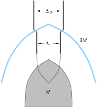
  Figure 2: A spherical star of mass $M$ undergoes collapse. Later, a spherical shell of mass $\delta{M}$ falls into the resulting black hole. While $\Delta_{1}$ and $\Delta_{2}$ are both isolated horizons, only $\Delta_{2}$ is part of the event horizon.

• The calculations of this paper have been performed using the connection dynamics framework [6] for general relativity. Although the boundary conditions take a particularly compact form in terms of these variables, we fully expect the classical framework can be formulated in terms of geometrodynamical variables. For passage to non-perturbative quantization [4], however, the connection variables seem essential.

• Our framework is closely related to an interesting body of ideas developed by Hayward [9]. Specifically, the isolated horizons introduced here are special cases of Hayward’s trapping horizons. The additional conditions imposed here were essential to our construction of Lagrangian and Hamiltonian frameworks, which in turn made it possible to carry out a non-perturbative quantization [4]. Our strategies for defining $\kappa$ and $M_{\Delta}$ are also different from those introduced in [9]. In particular, our definition yields the standard surface gravity for Reissner-Nordström black-holes, while the trapping gravity $\kappa$ of [9] does not.

• There are at least three directions in which our framework should be generalized to encompass other interesting situations. First, of course, rotating horizons should be allowed. This would entail constructing local expressions for the angular momentum and rotational velocity of an isolated horizon. At the present time, this appears to be mostly a technical matter as it requires one to weaken only the last boundary condition (on $n^{a}$) above. Second, Wald and collaborators have pointed out that the zeroth and first laws are largely theory independent in the stationary case [10]. It would be interesting to attempt to extend that analysis to isolated horizons. Finally, one can envisage genuinely dynamical processes. An extension of the framework along these lines would require non-trivial modifications but may be very useful, e.g., in numerical studies of black hole collisions.

Acknowledgments

We would like to thank participants at the Third Mexican School on Gravitation and Mathematical Physics at Mazatlán for numerous comments. This work was supported by the NSF grants PHY95-14240 and INT97-22514 and by the Eberly research funds of the Pennsylvania State University.

References

• [1] J.D. Bekenstein. Black Holes and Entropy. Phys. Rev. D7 (1973) 2333-2346.
• [2] J.M. Bardeen, B. Carter and S.W. Hawking. The Four Laws of Black Hole Mechanics. Commun. Math. Phys. 31 (1973) 161-170.
• [3] R.M. Wald. Quantum Field Theory in Curved Spacetime and Black Hole Thermodynamics. University of Chicago Press, Chicago, 1994.
• [4] A. Ashtekar, J. Baez, A. Corichi and K. Krasnov. Quantum geometry and black hole entropy. Phys. Rev. Lett. 80 (1998) 904-907.
A. Ashtekar, A. Corichi and K. Krasnov. Isolated Black Holes: The Classical Phase Space. To appear.
A. Ashtekar, J. Baez and K. Krasnov. Quantum Geometry of Isolated Horizons and Black Hole Entropy. To appear.
• [5] A. Ashtekar, C. Beetle and S. Fairhurst. The Mechanics of Isolated Horizons. To appear.
• [6] A. Ashtekar. Lectures on Non-Perturbative Canonical Gravity. World Scientific, Singapore, 1991.
A. Ashtekar. New variables for classical and quantum gravity. Phys. Rev. Lett. 57 (1986) 2244-2247.
A. Ashtekar. New hamiltonian formulation of general relativity. Phys. Rev. D36 (1987) 1587-1602.
• [7] L. Smarr. Mass Formula for Kerr Black Holes. Phys. Rev. Lett. 30 (1973) 71-73.
• [8] A. Ashtekar and M. Streubel. Symplectic geometry of radiative modes and conserved quantities at null infinity. Proc. R. Soc. Lond. A 376 (1981) 585-607.
A. Ashtekar. Radiative degrees of freedom of the gravitational field in exact general relativity. J. Math. Phys. 22 (1981) 2885-2895.
• [9] S.A. Hayward. General laws of black-hole dynamics. Phys. Rev. D49 (1994) 6467-6474.
• [10] R.M. Wald. Black Holes and Thermodynamics. In Black Holes and Relativistic Stars, ed. R.M. Wald. University of Chicago Press, Chicago, 1998.