On Accelerated Inertial Frames in Gravity and Electromagnetism

Abstract

When a charged insulating spherical shell is uniformly accelerated, an oppositely directed electric field is produced inside. Outside the field is the Born field of a uniformly accelerated charge, modified by a dipole. Radiation is produced.

When the acceleration is annulled by the nearly uniform gravity field of an external shell with a $1+\beta\cos\theta$ surface distribution of mass, the differently viewed Born field is static and joins a static field outside the external shell; no radiation is produced.

We discuss gravitational analogues of these phenomena. When a massive spherical shell is accelerated, an untouched test mass inside experiences a uniform gravity field and accelerates parallelly to the surrounding shell.

In the strong gravity régime we illustrate these effects using exact conformastatic solutions of the Einstein-Maxwell equations with charged dust. We consider a massive charged shell on which the forces due to nearly uniform electrical and gravitational fields balance. Both fields are reduced inside by the ratio of the $g_{00}$ inside the shell to that away from it. The acceleration of a free test particle, relative to a static observer, is reduced correspondingly. We give physical explanations of these effects.

Institute of Astronomy¹ and Clare College², Cambridge,

PPARC Senior Fellow on leave at School of Maths & Physics,

The Queen’s University³, Belfast. BT7 1NN,

Racah Institute of Physics⁴, The Hebrew University, Jerusalem,

Department of Theoretical Physics, Charles University⁵, Prague.

1 Introduction

When a massive spherical shell is accelerated a free body inside it experiences a parallel gravity field, i.e., the inertial axes inside accelerate. When the massive shell rotates the inertial axes inside also rotate. Weak versions of these inertia induction effects were discovered by Einstein (1912) in Prague[1] in the early variable-velocity-of-light version of his gravitational theories. He described them clearly in his 1913 letter to Mach[2]. In weak-field General Relativity he derives them in his book[3] but the non-Newtonian phenomena involved stretch the linearised theory to a doubtful level of approximation. Indeed the mass induction effect also discussed by Einstein was demonstrated to be a coordinate dependent effect by Brans (1962)[4].

Whereas a series of papers has been directed at the rotation of inertial frames within spheres, etc., Thirring (1918, 1921)[5], Lense & Thirring (1918)[6], Brill & Cohen (1966)[7], Lindblom & Brill (1974)[8], Embacher (1988)[9], Pfister & Braun (1985)[10], Klein (1993)[11], Lynden-Bell et al. (1995)[12], Katz et al. (1998)[13], less attention has been given to linear acceleration of the inertial frames within strongly relativistic spherical shells. This is perhaps because of the difficulty of producing strong accelerations in General Relativity without severe distortion of the problem to be solved. Near accelerating point masses the effects are complicated by the infall of the inertial frames and the gravomagnetic fields due to motion, but a few have been undeterred by these complications, e.g., Farhoosh & Zimmerman (1980)[15].

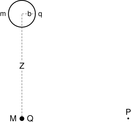
Figure 1: A spherical shell of radius $b$, mass $m$ and charge $q$ has a significant gravitational potential inside. It lies at coordinate distance $Z$ above a great mass $M$ with charge $Q$. They are of equal charge-to-mass-ratio, $\sqrt{G}$, and remain in equilibrium with the gravitational attractions balancing electrical repulsions. The acceleration of an uncharged test mass within the shell is compared to that at $P$ also distant $Z$ from $M$ but far from the shell $m$.

In continuation of our studies of Mach’s Principle & Machian effects within General Relativity[12, 16, 17, 18, 13], we demonstrate here the strong acceleration of the inertial frame within a massive charged spherical shell of mass $m$ and radius $b$, which is itself accelerated by a strong electric field. To do this we bring the system to rest by applying the equivalence principle and putting the system in an external gravity field $g$. Such a field can be provided by a distant massive body $M$ which can also be so charged that it supplies the electric field (Figure 1). To ensure that the principle of equivalence applies, the external tidal field of such a body across our spherical shell must be negligible. This can be achieved at constant internal potential by shrinking both the shell and its mass $m$ in proportion. We are interested in effects of order $gGm/(bc^{2})$ in acceleration. We fix $g$ and $m/b$. The tidal accelerations are of order $(GM/R^{3})b=g^{3/2}b(GM)^{-1/2}$ which can be made as small as we like by decreasing $b$ (and $m$) at constant ratio keeping $g$ and $M$ fixed.

The ratio of the accelerations we are interested in to those we wish to neglect is then $(Gm/bc^{2})(R/b)$ which we make as large as we like by taking $b\ll R$ with $m/b$ fixed. Notice we can do this with $g=GM/R^{2}$ held fixed at any value we like so we may study large accelerations and strong gravity $(Gm/bc^{2}\sim 1)$. We thus reduce the problem to statics and use the beautiful conformastatic solutions of Einstein’s equations for charged dust with balancing gravitational and electrostatic forces (see Appendix C). We show that the gravity field inside the massive charged spherical shell that sits balanced in such applied fields is smaller than the applied gravity field by the ratios of the $g_{00}$ which are themselves proportional to $[1+\sum Gm/(rc^{2})]^{-2}$. The problem may seem somewhat contrived in that it is not met in nature. We argue that it provides an ideal test-bed for study of strong linear dragging by large accelerations with strong relativistic effects and it is most unlikely that a simpler thought experiment can be devised.

However before entering the complications of general relativity it is wise to study the analogous problems in the electrodynamics of flat-space. For them we can determine truly time-dependent phenomena with the sphere initially at rest and only later given a uniform acceleration $\alpha$. For the transient behaviour see Appendix B. We encounter the oft discussed question whether a uniformly accelerated charge radiates and whether the equivalence principle applies to a radiating charge. This was well discussed by Fulton and Rohrlich (1960)[19] but even their excellent paper did not settle the question for some (Rosen 1962[20]). We have found it particularly interesting to draw the electric field lines of the Born (1909) solution [21] for a uniformly accelerated charge (see also Schott[22]) in several Lorentz frames including those in which the charged particle is momentarily at rest; see Figures 2a, b, c, d, e. The field lines are circles that intersect at the particle (Bondi & Gold 1955[23]). We join them far away to the initial Coulomb field of the fast moving particle before the steady deceleration brought it to near rest. In that field there is also a magnetic field with circular magnetic field lines around the direction the particle was moving. Such figures help us to envision how the Born solution describes the radiating field of an accelerated particle in the one case but can also describe the non-radiative static field of a particle held stationary in a uniform gravity field! As Boulware (1980)[24] showed, the principle of equivalence still holds in the region accessible to both the static and the coaccelerated observer, but does not hold beyond the event horizon of the coaccelerated observer who can see neither the radiation of the charge that is accelerated with him nor its effects.

2 The field of an accelerated charged spherical shell

For comparison to our sympathetic dragging calculations in gravity, we need the electromagnetic field inside a uniformly charged accelerated shell. Whereas the Born field of a point charge is well discussed, we give here the corresponding field inside and outside an accelerated charged shell. Inside the field rapidly $(2b/c)$ settles down to a uniform one but outside the propagation takes longer. Initially we calculate the field for short times only but the near field outside soon becomes that of a charge with a forward pointing electric dipole and no higher multipoles. These fit respectively the exact Born field and the exact field of uniformly accelerated dipole, both of which are known[25]. Thus our short-time calculation of the dipole moment tells us the coefficient of the dipole solution which should be added to the Born field to give the complete solution for the uniformly accelerated shell at all times.

We shall consider times close to the moment when the shell is stationary in our frame. Both charges and currents lie close to the shell $r=b$. The surface charge density is $Q/(4\pi b^{2})$ so we have a charge density

$$\rho={Q\over 4\pi b^{2}}\left(1-D{\partial\over\partial z}\right)\delta(r-b)\ ,$$

where $D(t)$ is the small displacement of the sphere at time $t$. Likewise the current on the sphere is

$${\bf j}={Q{\hat{\bf z}}\over 4\pi b^{2}c}\dot{D}\left(1-D{\partial\over\partial z}\right)\delta(r-b)\ .$$

Hats denote unit vectors.

To find the potentials we wish to solve

$$\Box^{2}\Phi=-4\pi\rho\ ,$$

$$\Box^{2}{\bf A}=-4\pi{\bf j}\ .$$

We first solve for the Green’s function $\chi$ such that

$$\Box^{2}\chi=-\delta(t-t^{\prime})\delta(r-b)\ .$$

Then

$$\Phi={Q\over b^{2}}\int\left(1-D(t^{\prime}){\partial\over\partial z}\right)\chi dt^{\prime}\ ,$$

and

$${\bf A}={Q{\hat{\bf z}}\over b^{2}c}\int{\dot{D}}(t^{\prime})\left(1-D(t^{\prime}){\partial\over\partial z}\right)\chi dt^{\prime}\ .$$

Now

$${1\over r}\left({\partial^{2}\over\partial r^{2}}-{1\over c^{2}}{\partial^{2}\over\partial t^{2}}\right)(r\chi)=-\delta(t-t^{\prime})\delta(r-b)\ .$$

The Green’s function $\chi$ which solves (2.5) and has only a retarded solution in $r\geq b$ is readily shown to be

$$\chi=-{bc\over 2r}\left\{{\Theta\left(t-t^{\prime}-{r+b\over c}\right)-\Theta\left(t-t^{\prime}+{r-b\over c}\right)\ ,\ r\leq b\atop\Theta\left(t-t^{\prime}-{r+b\over c}\right)-\Theta\left(t-t^{\prime}-{r-b\over c}\right)\ ,\ r\geq b}\right.$$

where ${\Theta}$ is 1 for a positive argument and zero otherwise. A detailed derivation of (2.9) is given in Katz et al. (1998)[13].

Returning to (2.6) and using ${\partial\over\partial z}f(r)={z\over r}{\partial\over\partial r}f$ we find

$$\Phi=Qb^{-2}\left[\int^{\infty}_{-\infty}\chi dt^{\prime}-{z\over r}{\partial\over\partial r}\int^{\infty}_{-\infty}D(t^{\prime})\chi(t^{\prime})dt^{\prime}\right]\ .$$

For a uniformly accelerated sphere, $D(t^{\prime})={\textstyle{1\over 2}}\alpha t^{\prime 2}$, and the integrals are readily evaluated to give

$$\Phi=\left\{{Qb^{-1}\left(1-{1\over 3}\alpha c^{-2}z\right)\quad\ \,{\rm inside,\ i.e.,}\ |{\bf r}-{1\over 2}\alpha t^{2}{\hat{\bf z}}|\leq b\atop Qr^{-1}\left\{1+{1\over 2}\alpha c^{-2}z\left[\left(c^{2}t^{2}+{1\over 3}b^{2}\right)r^{-2}-1\right]\right\},\ \ r\geq b}\right.\ .$$

Returning to (2.7) we see that the $\dot{D}D$ term is quadratic in the acceleration $\alpha$ so the first term will suffice when $\alpha bc^{-2}\ll 1$. For an acceleration of 1g this means $b$ much smaller than a light year $\sim 10^{18}$ cm! Evaluating ${\bf A}$ for a general $D$ we find

$${\bf A}=-{\textstyle{1\over 2}}Q{\hat{\bf z}}b^{-1}r^{-1}\left\{{D\left(t-{r+b\over c}\right)-D\left(t+{r-b\over c}\right)\qquad r\leq b\,,\atop D\left(t-{r+b\over c}\right)-D\left(t-{r-b\over c}\right)\qquad r\geq b\,,}\right.$$

or for $D={\textstyle{1\over 2}}\alpha t^{2}$

$${\bf A}=Q\alpha c^{-2}{\hat{\bf z}}\left\{{b^{-1}(ct-b)\qquad r\leq b\atop r^{-1}(ct-r)\qquad r\geq b}\right.\ .$$

The fields are readily derived from ${\bf E}=-c^{-1}{\dot{\bf A}}-\mbox{\boldmath$\nabla$}\Phi$. Inside the uniformly accelerated sphere we have, writing $a=c^{2}/\alpha$,

$${\bf E}_{\rm in}=-{2\over 3}Q(ab)^{-1}{\hat{\bf z}}\qquad r\leq b\ ,$$

and outside

$$\halign{\hbox to\displaywidth{$\hfil\displaystyle#\hfil$}\cr 0.0pt{\hfil$\displaystyle{\bf E}_{\rm out}=Qr^{-2}\left\{1-{\textstyle{1\over 2}}(z/a)\left[1-r^{-2}(3c^{2}t^{2}+b^{2})\right]\right\}{\hat{\bf r}}-\cr 0.0pt{\hfil$\displaystyle\hfill-{\textstyle{1\over 2}}Q(ar)^{-1}\left[1+{\textstyle{1\over 3}}r^{-2}(3c^{2}t^{2}+b^{2})\right]{\hat{\bf z}}\ \ \ \ ,\ \ \ \ \sqrt{ab}\gg r\geq b\ .\hfill{(2.15)}\cr}}}$$

We have performed our calculation under the assumption that the movement of the sphere during the time considered is much less than the radius of the sphere. Thus the result is only valid provided the times involved obey

$${\textstyle{1\over 2}}\alpha t^{2}\ll b\ .$$

During this time the signal will propagate to $r=ct$ so the solution is only valid where $r^{2}\ll 2bc^{2}\alpha^{-1}=2ab$. To get the field at greater distances we may refer to Born’s solution for the field of a point charge which is uniformly accelerated in its own frame so its position is given by

$$z=\sqrt{a^{2}+c^{2}t^{2}}-a={\overline{z}}-a\ .$$

This is given in Appendix A.

We initially expected the external field of our accelerated sphere on which the charge density was frozen, to match exactly the “small acceleration” (large $a$) limit of the Born solution. However the presence of $b^{2}$ terms in (2.15) shows that this cannot be the case since in Born’s solution there is no $b$. Indeed those terms show that our accelerated sphere has a dipole of moment ${\bf P}={\textstyle{1\over 6}}Q(b^{2}/a){\hat{\bf z}}$. Bičák and Muschall (1991)[25] showed how to get the exact solutions for uniformly accelerated multipoles by differentiating Born’s solution with respect to $a$. Putting their dipole equal to the above ${\bf P}$ and adding the result to Born’s solution gives the exact external solution for our uniformly accelerated sphere, see (2.17), etc. below. Of course if we set $b=t=0$ our external fields fit the Born solution including terms of order $1/a$ but not when $r>a$. The physical origin of our forward pointing dipole is interesting. Our ${\bf E}$ field arises as it should from a spherically symmetrical distribution of surface charge. In the Born solution the field-lines droop under their acceleration-induced weight (see Fig. 2b). By demanding that our sphere be of uniform surface density we have demanded no droop out to $r=b$. The droop of the Born field lines is therefore offset by the forward pointing dipolar field we have found.

If we cut Born’s solution at $r=b$ we may replace the inside with a charged shell but, its internal ${\bf E}$ field is not our $-{\textstyle{2\over 3}}Q(ab)^{-1}{\hat{\bf z}}$ but another uniform field whose coefficient is $-{\textstyle{1\over 2}}$ in place of $-{\textstyle{2\over 3}}$. The reason for this difference is that the surface charge density on a sphere that gives the Born field outside is not uniform but rather $\sigma={Q\over 4\pi b^{2}}(1-{\textstyle{1\over 2}}{b\over a}\cos\theta)$. It is the internal field of this non-uniform charge density with excess charge at the bottom that reduces the internal field strength from ${\textstyle{2\over 3}}$ to ${\textstyle{1\over 2}}$. Thus our ‘exact’ solution for a uniformly charged uniformly accelerated sphere is not Born’s field outside, but is given by

$${\left.\Phi=\left[1+{1\over 3}b^{2}\left({\partial\over\partial a^{2}}\right)_{{\overline{z}}}\right]\Phi^{B}(R,{\overline{z}},t,a^{z})\atop\ \ {\bf A}={\hat{\bf z}}\left[1+{1\over 3}b^{2}\left({\partial\over\partial a^{2}}\right)_{{\overline{z}}}\right]A^{B}(R,{\overline{z}},t,a^{2})\right\}}\ ,$$

where, to allow steady uniform acceleration, we have to take $b\ll a=c^{2}/\alpha$, and $\Phi^{B}$ and $A^{B}$ are given in Appendix A.

Inside the sphere, which becomes Lorentz contracted into an oblate spheroid away from $t=0$, the electric field is always given by (2.14) with no magnetic field there. These properties follow from Lorentz transformation of our $t=0$ field. We discuss the transients when the shell starts from rest in Appendix B.

Born’s field is static in uniformly accelerated axes.

3 Gravity in Accelerated Shells

In weak field theory, Einstein considered a spherical shell of mass $m$ and radius $b$ that was weakly accelerated by some unspecified forces and looked at the metric inside the shell. We wish to accelerate a massive shell quite rapidly and we need to specify some way of doing it because the stresses involved will produce their own gravity. We therefore consider a uniformly charged insulating massive spherical shell in an electric field so that every element will accelerate uniformly without any acceleration-induced stresses. Einstein using his 1912 theory[1] found a uniform gravity field of strength ${fGm\over c^{2}b}\,\mbox{\boldmath$\alpha$}$ within his accelerating shell, where $f$ was $3/2$ using coordinate time. However in his 1955 book[3] he gives the weak field relativistic formulae in the de Donder gauge. Evaluating these, including retardation in the potential, gives an ${\dot{\bf A}}$ term – $4\times$ the analogous electrical one and a ${\mbox{\boldmath$\nabla$}}\Phi$ term equal and opposite to the electrical one. So we get from Einstein’s weak field formulae $f=11/3$. So we should expect a free test body inside our shell to accelerate in sympathy but less rapidly than the shell itself. However time-dependent problems in general relativity are difficult, so rather than solving a difficult problem we shall use the principle of equivalence to reduce it to an easy one. The acceleration of the whole shell is equivalent to a uniform gravity field imposed from outside. If ${\bf E}$ is the accelerating electric field and $q$ and $m$ are the charge and mass of the shell, then the upward acceleration is $\mbox{\boldmath$\alpha$}=q{\bf E}/m$ as shown in Bičák 1980[26]. The extra ‘fictitious’ downward gravity field that appears to a coaccelerated observer is ${\bf g}=-\mbox{\boldmath$\alpha$}$, and the principle of equivalence is that the metric felt by such an observer will be the same as that static metric felt when the extra gravity field, ${\bf g}$, is really present. To generate such a real gravity field we place a very large mass $M$ at a large distance $Z$ down the z axis such that the gravity field due to it is just ${\bf g}$ that is $g\simeq GM/Z^{2}$. We may also use this mass to generate the electric field ${\bf E}$ by giving it a charge $Q=EZ^{2}$. Then the gravitational attraction of $m$ by $M$ exactly cancels their electrical repulsion so the whole system is static and at least classically $qQ=GmM$. Because it makes even the general relativity easy we shall take both the sphere and the large $M$ to have equal charge to mass ratio so $q/m=Q/M=\sqrt{G}$. That is each has the charge/mass ratio of the extreme Reisner-Nordström black hole. To attain bodies with $Q=\sqrt{G}M$ we put together $N(1-f)$ hydrogen atoms and $Nf$ protons to give $Q=fNe$ and $M\simeq Nm_{H}$. Then $QG^{-1/2}M^{-1}=eG^{-1/2}m^{-1}_{H}f=f/9\times 10^{-19}$, so we must choose $f=9\times 10^{-19}$ to get balanced electrical and gravitational forces. This gives about $10^{18}$ neutral hydrogens per proton, implying a charge of 1 Coulomb on $1.18\times 10^{13}$gm or about $1.7\times 10^{20}$ Coulombs on a solar mass which would give it a potential of $2.5\times 10^{19}$ volts, far more than realistic values.

With such $Q/M$ values we see that each element of the original spherical shell and the large mass $M$ is in balance with the electric and gravitational forces neutralising one another. But that is just the condition required for the metric to be one of what Synge[27] calls conformastatic spaces, whose metrics take the delightfully simple form

$$ds^{2}=V^{-2}dt^{2}-V^{2}(dx^{2}+dy^{2}+dz^{2})\ ,$$

where $V=V(x,y,z)$.

Take any function $V$ that $\rightarrow 1$ at infinity and satisfies $V^{-3}\nabla^{2}V\leq 0$. Then defining a proper energy density $\rho$ by

$$V^{-3}\nabla^{2}V=-{\textstyle{1\over 2}}\kappa\rho\ ,$$

where $\kappa=8\pi G/c^{4}$ and

$$\nabla^{2}={\partial^{2}\over\partial x^{2}}+{\partial^{2}\over\partial y^{2}}+{\partial^{2}\over\partial z^{2}}\ ,$$

we find that the metric solves the Einstein-Maxwell equations with electric field ${\bf E}=(G)^{1/2}\mbox{\boldmath$\nabla$}V^{-1}$. Here $\mbox{\boldmath$\nabla$}=\left({\partial\over\partial x},{\partial\over\partial y},{\partial\over\partial z}\right)$. Since these solutions are more commonly described for arbitrary point masses with the appropriate charges we give a brief outline of them in Appendix C. Now $\nabla^{2}$ is an operator in $(x,y,z)$ space while $\rho$ is a proper energy density of charged dust. To find the corresponding coordinate density of dust we set

$$\rho\,d{(\rm Volume)}\ =\rho V^{3}dxdydz=\rho_{c}dxdydz\ ,$$

so $\rho_{c}(x,y,z)=\rho V^{3}$, hence

$$\nabla^{2}V=-{\textstyle{1\over 2}}\kappa\rho_{c}\ .$$

For our problem we need the conformastatic metric of a spherical shell with a distant charged mass, see Fig. 1. Taking relativistic units $G=c=1$,

$$V=\left\{{{M\over R}+{m\over r}+1\qquad r\geq b\atop{M\over R}+{m\over b}+1\qquad r\leq b}\right\}\ ,$$

where $R$ and $r$ are the $x,y,z$ coordinate distances from $M$ and $m$. Far away from both shells, $g_{00}=V^{-2}=1-2M/R-2m/r$.

Any test mass with charge to mass ratio $\sqrt{G}$ will be in static equilibrium with balancing gravitational and electric forces if placed at any point in such a metric. However we shall be concerned with the motion of an uncharged test mass. Placed well away from the spherical shell $m$ and at the same distance $Z$ from $M$, Figure 1, a test mass will accelerate towards $M$ with initial acceleration $|{\bf g}|={M\over Z^{2}}$ but will the acceleration of a test mass placed inside the spherical shell be greater or less than $|{\bf g}|$?

Relative to freely falling axes the shell is accelerated upwards by the electric field so we expect a test mass inside to have an acceleration in sympathy. Thus relative to static axes we expect the acceleration of the test mass within the sphere to be smaller than $|{\bf g}|$. However in strong field general relativity there are other effects that work in the same direction. What should we compare, coordinate accelerations, $g_{c}=\left|d^{2}{\bf r}/dt^{2}\right|$, proper accelerations, $g_{p}=\left|d/d\tau\left(Vd{\bf r}/d\tau\right)\right|$, or proper length accelerations using universal coordinate $t$-time, $g_{u}=\left|d/dt\left(Vd{\bf r}/dt\right)\right|$? Here ${\bf r}$ stands for $(x,y,z)$. One could argue that because time runs slowly at greater gravitational potentials we expect a slower apparent acceleration in $t$-time irrespective of any sympathetic acceleration effect. The equations of geodesic motion in proper time $\tau$ are

$$d/d\tau(V^{2}d{\bf r}/d\tau)=(2V^{2}\varepsilon^{2}-1)\mbox{\boldmath$\nabla$}{\rm ln}V$$

and the conserved specific energy is $\varepsilon=V^{-2}{\dot{t}}$, where a dot means $d/d\tau$. Since $d\tau$ is $ds$ along the particle’s motion,

$$V^{-2}\,{\dot{t}}^{2}-V^{2}\,{\dot{\bf r}}^{2}=1\ .$$

From the above we find expressions for ${\bf g}_{c}\,,{\bf g}_{p}$ and ${\bf g}_{u}$. For a body released from rest $(\varepsilon=V^{-1})$ the initial accelerations are

$${\bf g}_{c}=V^{-5}\mbox{\boldmath$\nabla$}V\ ,$$

$${\bf g}_{p}=V^{-2}\mbox{\boldmath$\nabla$}V\ ,$$

$${\bf g}_{u}=V^{-4}\mbox{\boldmath$\nabla$}V\ .$$

Each of these measures of acceleration is affected by the value of $V$ as well as its gradient. So, if the potential, $m/b$, due to the shell is large, the acceleration of the body inside the shell will be much reduced compared with that of another body far from $m$ but at the same distance from $M$. Whereas in (3.7) and (3.9) much of this difference can be attributed to slowed time that does not account for the result (3.8) where such effects are eliminated by using time as measured on the particle. In these conformastatic models there is an invariant definition of the gravity field. All are agreed that the systems are in balance and that any test particle of charge to mass ratio $\sqrt{G}$ can be placed anywhere in such a metric and will be in equilibrium. Thus the electric field in the static frame (which is invariantly defined) must be equal and opposite to the gravitational field ${\bf g}$. Since the electric field is $\mbox{\boldmath$\nabla$}(V^{-1})$, the gravitational field is $-\mbox{\boldmath$\nabla$}(V^{-1})=V^{-2}\mbox{\boldmath$\nabla$}V$. So this invariant definition of the gravity field leads us back to ${\bf g}_{p}$. Comparing those accelerations inside the shell to those far from it we have

$$(g_{p})_{{\rm in}}/(g_{p})_{{\rm out}}=E_{{\rm in}}/E_{{\rm out}}=(V_{{\rm in}}/V_{{\rm out}})^{-2}=\left({1+{M\over Z}\over 1+{M\over Z}+{m\over b}}\right)^{2}\ ,$$

so if $m/b$ is larger than $1+M/Z$ the reduction can be very large. It is important to notice here that $b$ can be as small as we like; $b=0$ corresponds to an extreme Reinsner Nordström black hole. Indeed as shown by Hartle & Hawking 1972[28] our coordinate radius $r$ is related to Schwarzschild’s coordinate $r_{s}$ by $r=r_{s}-m$.

We have argued above that this reduction of the test mass’s acceleration is due to its sympathetic dragging produced by the acceleration of the surrounding shell (relative to freely falling axes). However, let us now take the view of the static observer at infinity; the shell is not accelerating at all. It then appears strange that this zero acceleration can have any effect. Indeed Einstein attributed such effects that did not involve his ‘vector potential’ ${\bf A}$ not to any sympathetic dragging but to mass induction – an increase of inertia due to the presence of the surrounding sphere. The calculation above shows that the reduced gravity field, as seen in the static frame, is parallelled by the reduction of the electric field. We do not attribute the latter to any change of charge, so the former should not be attributed to Einstein’s mass induction but is better viewed as a “diagravitational” effect of the potential, similar to a dielectric effect, but reducing both the electric and the gravitational fields inside the medium. Evidently the sympathetic dragging interpretation in the freely falling frame is equivalent to this diagravitational effect in the static frame.

4 Static Charge in a Conformastatic $(1+\beta\cos\theta)$ Weighted Shell

The method of the last section can be used to give a finite region of almost uniform gravity field within a single spherical shell of total mass $M$ with all charges equal to $\sqrt{G}$ times all masses. Take

$$V=\left\{{1+{M\over r}-Ab^{3}r^{-2}\cos\theta\qquad r\geq b\atop\ \ 1+{M\over b}-Ar\cos\theta\qquad\quad\ r\leq b}\right\}\ \ ,$$

where $A$ is a constant. Inside, ${\mbox{\boldmath$\nabla$}}V$ is constant but the gravity field $g$ varies at order $A^{2}$ as it is $V^{-2}{\mbox{\boldmath$\nabla$}}V$. The coordinate surface density of mass on the shell, $\sigma_{c}$, is given by integrating (3.3) across the shell

$$4\pi\sigma_{c}=4\pi V^{-2}\sigma=Mb^{-2}-3A\cos\theta\ ,$$

where we have written $\sigma$ for the proper surface density per unit proper area; the metric is

$$ds^{2}=V^{-2}dt^{2}-V^{2}\left[dr^{2}+r^{2}(d{\hat{\bf r}})^{2}\right]=V^{-2}dt^{2}-V^{2}\left(dx^{2}+dy^{2}+dz^{2}\right)\ .$$

For $r\leq b$ the transformation $t=K{\overline{t}}$, $K^{-1}=1+M/b$, $x=K{\overline{x}}(1+{\overline{A}}\,{\overline{z}})$, $y=K{\overline{y}}(1+{\overline{A}}\,{\overline{z}}),z=K\left[{\overline{z}}+{1\over 2}{\overline{A}}\left({\overline{z}}^{2}-{\overline{x}}^{2}-{\overline{y}}^{2}\right)\right],{\overline{A}}=K^{2}A$ yields for small $A$ $(A^{2}b^{2}$ neglected)

$$ds^{2}=\left(1+{\overline{A}}\,{\overline{z}}\right)^{2}d{\overline{t}}^{2}-\left(d{\overline{x}}^{2}+d{\overline{y}}^{2}+d{\overline{z}}^{2}\right)\ ,$$

which is flat space in accelerated axes (cf[26]) and ${\overline{A}}$ is identified with our former $a^{-1}$. The physical electric field in our conformastatic metric is ${\bf E}=\mbox{\boldmath$\nabla$}V^{-1}$ everywhere and this $\nabla$ is the coordinate $\nabla$. Writing it in terms of the physicists gradient per unit distance $\mbox{\boldmath$\nabla$}_{p}=V^{-1}\mbox{\boldmath$\nabla$}$ so ${\bf E}=-\mbox{\boldmath$\nabla$}_{p}\,{\rm ln}V$ and ln$V$ is the physicists potential (in volts say). Now this is invariant for purely spatial coordinate changes like that above. Hence the potential due to adding a small charge $q$ at the origin (with the mass appropriate for the conformastat) is $q/(rV)$. Rewriting $r$ and $V$, $r=K{\overline{r}}\left(1+{1\over 2}{\overline{A}}\,{\overline{z}}\right)$ and $V=K^{-1}\left(1-{\overline{A}}\,{\overline{z}}\right)$ we have the potential to order ${\overline{A}}=1/a$,

$$\Phi={q\over{\overline{r}}}\left(1+{1\over 2}\,{{\overline{z}}\over a}\right)\ ,$$

which agrees with Born’s field in accelerated axes to this order.

The field ${\bf E}$ is still given in conformastatic coordinates by

$${\bf E}=\mbox{\boldmath$\nabla$}\left(\delta{1\over V}\right)=-\mbox{\boldmath$\nabla$}\left(qr^{-1}V^{-2}\right)\ .$$

Outside the field is still static and given by (4.6) but of course the external form of $V$ must be used there.

5 Radiation and the Equivalence Principle

In the last section we had a static charge in the gravitational field of a shell. It produces the Born field locally but no radiation. In Section 2 we had an accelerated charged sphere in flat space which produced a ‘Born’ field with radiation at large distances.

Here we analyse the electromagnetic field of a particle which after moving uniformly at high speed has decelerated to rest and will continue its constant acceleration until it disappears whence it came. We draw the field lines and show that it radiates in a region inaccessible to the coaccelerating observer which does not exist for the static charge in the shell. Then we consider the corresponding problem for accelerated masses producing gravitational radiation.

Figure 2a is a space-time diagram with time plotted to the left and $z$ upwards. The reason for $z$ up will soon appear. $t$ is plotted leftwards so that creatures of habit can recover their familiar space-time diagram by rotating the page by 90^∘. The charged particle is confined to the line $x=y=0$ and at $P$ it is moving downwards at a little less than the light velocity. However it is uniformly accelerated upwards, for $t\geq t_{0}$, so that the acceleration felt in the momentary rest frames is constant thereafter. This acceleration slows it to momentary rest at $O$ before it continues to accelerate upwards to $O^{\prime}$ and beyond. The space-time diagram is drawn using coordinates and time appropriate for its rest moment at $O$. Prior to arrival at $P$ the particle was moving downwards at constant velocity so the acceleration only started at $P$. It is clear from Fig. 2a that a coaccelerated observer who moves with the particle can never see anything in the lower left of the diagram below the shaded line, ${\overline{z}}=z+a=t$. Light from such points can never reach any point of the hyperbola $POO^{\prime}$. Thus the region ${\overline{z}}<t$ is beyond his horizon which is at $\overline{z}=t$. Likewise nothing done by such an observer can influence the region below $\overline{z}=-t$ unless it was already done before the particle started to accelerate (and before the particle crossed out of that region at $S$).

Figure 2b shows a perpendicular slice of Minkowski space containing the $x,z$ plane through $O$. The lines of force of the Born electric field are a set of circles through $O$ whose centres lie on $z=-a$, (i.e., $\overline{z}=0$). $P^{\prime}$ is the same point of space as $P$ but at the later time (as reckoned in this Minkowski frame). Beyond the circle of radius $t_{0}$ around $P^{\prime}$ there has not been time for the field to feel the acceleration that started at $t_{0}$ so the field is the old field that there would have been had the particle continued its prior uniform motion to $Q$. Now the field of a fast moving particle is a radial electric field flattened by Lorentz contraction along its direction of motion (See Fig. 2d) and accompanied by circles of magnetic field around the direction of motion; so this is the field centred on $Q$ beyond $t_{0}$ from $P^{\prime}$. The field lines of the Born field in Figure 2b droop because in the accelerated frame that travels with the particle there is an apparent gravity field downwards and gravity acts on the field’s energy and stresses. There is no magnetic field in the Born region of this diagram because we have taken the time symmetric moment, $t=0$, when the particle is momentarily at rest. Then the Born fields in both the Minkowski and the accelerated frames coincide. There is no transient between the Born field and the fast particle’s field, merely the circular front (see Appendix B). It is of interest to see how the field in Figure 2b evolves at later times. We draw it in two instructively different ways when the particle has moved on to $O^{\prime}$. It seems natural to take moving axes and draw the field in the frame in which the particle at $O^{\prime}$ is at rest. We then get Figure 2c in which the Born part of the field extends farther, the front is now closer to $X$ and the original fast particle’s field beyond it is more Lorentz contracted since in these axes the particle at $P$ was moving faster. It is instructive to see what cut in space-time corresponds to this diagram. It is $O^{\prime}X$ in Figure 2a. Thus the set of such pictures in which the Born field is static are a set of cuts through $X$. These diagrams only cover the upper and lower of the four sectors through $X$, the others are unrepresented so far.

On the cut $PX$ the Born region has shrunk to zero and $P$ is reduced to rest so the field is just that of a static charge. We have not drawn that figure. However we have drawn in Figure 2d the field lines of the rapidly moving unaccelerated charge corresponding to the slice $YP$ through Figure 2a at time $t_{0}$. This shows the Lorentz contracted Coulomb field and the associated magnetic field in circles about the motion. The corresponding slice at time $t=0$ is of course Figure 2b. In Figure 2e we draw the vertical slice through $O^{\prime}$. We now reach into the radiation zone invisible to coaccelerating observers and indeed $Q$ has now moved into that zone at $Q^{\prime\prime}$. The electric field lines are again circles through $O^{\prime}$ centred on $\overline{z}=0$ but now they are accompanied by magnetic fields in circles and start to converge again before joining the old field of the fast moving particle outside the circular front. Some may feel surprised that the fields change discontinuously on this front although the potentials are of course continuous. One might have expected that discontinuous changes in field would always be accompanied by surface densities of charge or current but in fact such changes can happen on null surfaces as is the case here. An even more extreme configuration is illustrated in Gull et al.[29] among their pictures of various electromagnetic fields. To see the radiation in the Born field one sets $t=u+r$ which brings one clearly into the “radiative zone” of Figure 2a and takes the asymptotic form at large $r$ with $u$ fixed. This gives

$${\bf E}=qa^{2}{{\hat{\bf r}}\times({\hat{\bf r}}\times{\hat{\bf z}})\over r(u^{2}+a^{2}\sin^{2}\theta)^{3/2}}\ ,$$

$${\bf B}=qa^{2}{{\hat{\bf z}}\times{\hat{\bf r}}\over r(u^{2}+a^{2}\sin^{2}\theta)^{3/2}}\ .$$

Thus ${\bf E}$ and ${\bf B}$ are perpendicular and perpendicular to ${\hat{\bf r}}$, and fall only as $r^{-1}$ which demonstrates the radiative field in this region.

The only explicit solutions of Einstein’s equations available today that represent radiative gravitational fields of finite sources have much in common with the Born solution in electrodynamics. These “boost-rotation symmetric” space-times have two symmetries exhibited by the axial Killing vector, and the boost Killing vector which, in appropriate coordinates, has the flat-space form, $\zeta^{\alpha}=(z,0,0,t)$. The Born solution has the same symmetries. The boost-rotation symmetric space-times represent the fields of “uniformly accelerated particles” which may be black holes as is the case for the C-metric. The “sources” of the accelerations are strings along the z-axis. Analogously to the Born solution, gravitational waves are found in the region $|t|>|z|$ where the boost Killing vector is space-like. In the region $|z|>|t|$, the metrics can be transformed into static forms – the sources are at rest in uniformly accelerated reference frames, again in full analogy with the Born case. The radiative character of the solutions is best seen on asymptotic forms of the Riemann tensor at null infinity. The Riemann tensor falls-off as $r^{-1}$, in the analogy with the “radiative fall-off” of electric and magnetic fields at $r\rightarrow\infty$ with $u$ fixed, given in (5.1), (5.2). In addition, the analogous features of fields due to some specific exact boost-rotation symmetric space-times and uniformly accelerated charges appear even in the radiation patterns and total rates of radiation, as first demonstrated many years ago[30].

The structure of general boost-rotation symmetric space-times was analysed much later by Bičák & Schmidt (1989)[31]. In the review “Radiative space-times: exact approaches”[32], the main properties and applications of the boost-symmetric space-times are summarised.

Appendix A Born’s Solution $(c=1)$

Born’s solution is written in terms of $R^{2}=x^{2}+y^{2}$ and $\overline{z}=z+a$. We put

$$\zeta=\left[\left(a^{2}+t^{2}-R^{2}-\overline{z}^{2}\right)^{2}+4a^{2}R^{2}\right]^{1/2}\ .$$

The Born potentials are

$$\Phi^{B}=q[\overline{z}(R^{2}+\overline{z}^{2}+a^{2}-t^{2})\zeta^{-1}-t]/(\overline{z}^{2}-t^{2})$$

$${\bf A}^{B}={\hat{\bf z}}A^{B}={\hat{\bf z}}q[t(R^{2}+\overline{z}^{2}+a^{2}-t^{2})\zeta^{-1}-\overline{z}]/(\overline{z}^{2}-t^{2})\ .$$

From these follow the fields

$${\bf E}^{B}=4a^{2}q\zeta^{-3}[-(a^{2}+t^{2}+R^{2}-{\overline{z}}^{2}){\hat{\bf z}}+2R{\overline{z}}{\hat{\bf R}}]\ ,$$

$${\bf B}^{B}=8a^{2}q\zeta^{-3}Rt\,{\hat{\bf z}}\times{\hat{\bf R}}\ ,$$

where ${\hat{\bf R}}$ and ${\hat{\bf z}}$ are unit vectors along $(x,y,0)$ and $(0,0,1)$ respectively.

To evaluate the dipolar contribution to (2.17) we need

$$(\partial\zeta^{-1}/\partial a^{2})_{\overline{z}}=-\zeta^{-3}(a^{2}+t^{2}+R^{2}-\overline{z}^{2})$$

$$(\partial\Phi^{B}/\partial a^{2})_{\overline{z}}=-2q\overline{z}\zeta^{-3}(t^{2}+a^{2}-R^{2}-\overline{z}^{2})$$

$$\partial A^{B}/\partial a^{2}=(ct/\overline{z})\,\partial\Phi^{B}/\partial a^{2}\ .$$

Since dipoles are generated by small shifts we have following Bičák & Muschall (1980)[25]

$$\Phi=\Phi^{B}+{{\bf P}\cdot{\hat{\bf z}}\over Q}\left({\partial\Phi^{B}\over\partial a}\right)_{\overline{z}}=\Phi^{B}+{\textstyle{1\over 3}}b^{2}\left({\partial\Phi^{B}\over\partial a^{2}}\right)_{\overline{z}}$$

with an analogous formula for ${\bf A}$. Thus the total external potential $\Phi$ is given by multiplying (A7) by ${\textstyle{1\over 3}}b^{2}$ and adding it to (A2). ${\bf A}$ is constructed similarly.

Appendix B Electromagnetic Transients

It is of interest to see how the fields arise when the sphere is at rest initially and is then uniformly accelerated from $t=0$ onwards. To find such solutions, we put $D={\textstyle{1\over 2}}\alpha t^{2}\Theta(t)$ and evaluate our formulae as before. We find from (2.10) and (2.13) that for $r\leq b$, $\Phi$ takes the values

$$\left\{\begin{array}[]{ll}\!\!\!Qb^{-1}&\!\!\!\ \,t\leq{b-r\over c}\\ \!\!\!Qb^{-1}\left\{1+{\textstyle{1\over 12}}\alpha czr^{-3}\left(-3{r\over c}+t+{r-b\over c}\right)\left(t+{r-b\over c}\right)^{2}\right\}&\!\!\!\ \,{b+r\over c}\geq t\geq{b-r\over c}\\ \!\!\!Qb^{-1}\left(1-{\textstyle{1\over 3}}\alpha zc^{-2}\right)&\!\!\!\ \,t\geq{b+r\over c}\end{array}\!\!\!\right\}$$

and

$${\bf A}=\left\{\begin{array}[]{ll}0&\ \ \ t\leq{b-r\over c}\\ -{\textstyle{1\over 4}}Qb^{-1}{\hat{\bf z}}\alpha r^{-1}\left(t+{r-b\over c}\right)^{2}&\ \ \ {b+r\over c}\geq t\geq{b-r\over c}\\ -Qb^{-1}{\hat{\bf z}}\alpha c^{-2}(ct-b)&\ \ \ t\geq{b+r\over c}\end{array}\right\}$$

while for $r\geq b$, $\Phi$ takes the values

$$\left\{\begin{array}[]{ll}Qr^{-1}&\ \ \ t\leq{r-b\over c}\\ Qr^{-1}\left\{1-{\textstyle{1\over 12}}\alpha czb^{-1}r^{-2}\left({3r\over c}+t-{r-b\over c}\right)\left(t-{r-b\over c}\right)^{2}\right\}&\ \ \ {r+b\over c}\geq t\geq{r-b\over c}\\ Qr^{-1}\left\{1-{\textstyle{1\over 2}}\alpha c^{-2}z\left[1-{(3c^{2}t^{2}+b^{2})\over 3r^{2}}\right]\right\}&\ \ \ t\geq{r+b\over c}\end{array}\right\}$$

and

$${\bf A}=\left\{\begin{array}[]{ll}0&\ \ \ t\leq{r-b\over c}\\ -{\textstyle{1\over 4}}Qr^{-1}{\hat{\bf z}}\alpha b^{-1}\left(t-{r-b\over c}\right)^{2}&\ \ \ {r+b\over c}\geq t\geq{r-b\over c}\\ -Qr^{-1}{\hat{\bf z}}\alpha c^{-2}(ct-r)&\ \ \ t\geq{r+b\over c}\end{array}\right\}\ .$$

Evidently the internal potentials and fields settle down to their steady state after a transient that lasts for a period of $2b/c$. However these transients travel outwards with the velocity of light and are seen later at greater distances as we would expect. Transients for other starting times can be found by the Lorentz transformation which reduces the starting velocity to rest. We may apply similar considerations to the case $b=0$, a point charge started from rest. The field of a static or uniformly moving charge changes to Born’s field with a transient that lasts for zero time at each point and travels outward with the velocity of light.

Appendix C Conformastats

These static space-times, so named by Synge[27], have conformally flat spatial metrics. The Schwarzschild solution is a conformastat but the best known examples are electrovacuum solutions due to Majumdar[33] and Papapetrou[34] representing extreme Reissner-Nordström black holes in arbitrary positions in static equilibrium. Less known (not explicitly included in[35]) are the conformastatic space-times with charged dust, in which the ratio of the charge to mass densities $\rho_{e}/\rho$, is everywhere $\pm\sqrt{G}$. (In Section 3, we took $\rho_{e}/\rho=+\sqrt{G}$.) As in Newtonian physics the material is in equilibrium because the mutual gravitational attractions are balanced by the electrical repulsions. This class of exact solutions was studied, for example, by Das[36], Bonnor and Wikramasuriya[37], and Bonnor[38]. We did not, however, find a clear simple derivation of the general solutions of this type. Following Synge[27], consider the particular conformastat form of the metric,

$$ds^{2}=V^{-2}dt^{2}-V^{2}(dx^{2}+dy^{2}+dz^{2})\ ,$$

where $V=V(x,y,z)$. As a source, take a static electric field described by potential $\phi(x,y,z)$ and a charged dust with static proper matter and charge densities $\rho(x,y,z)$ and $\rho_{e}(x,y,z)$ (not initially assumed to be equal), in the coordinates of the metric (C1).

Therefore, the energy-momentum tensor of the dust is $T^{\mu\nu}\,({\rm dust})\ =\rho U^{\mu}U^{\nu}$, and its current density is $j^{\mu}=\rho_{e}U^{\mu}$, where $U^{\mu}=\delta^{\mu}_{0}V$. The electromagnetic field is described by $F_{\mu\nu}=A_{\nu,\mu}-A_{\mu,\nu}$, with $A_{\mu}=(\phi,0,0,0)$, and the standard energy-momentum tensor

$$T_{\mu\nu}({\rm em})\ ={1\over 4\pi}\left(-F_{\mu}^{\sigma}F_{\nu\sigma}+{\textstyle{1\over 4}}g_{\mu\nu}\,F_{\rho\sigma}F^{\rho\sigma}\right)\ .$$

The Ricci tensor components for the metric (C1) read

$$R_{ij}=-2V^{-2}V,_{i}V,_{j}+\delta_{ij}V^{-1}(-\nabla^{2}V+V^{-1}\nabla V\nabla V)\ ,$$

$$R_{00}=V^{-5}(V^{-1}\nabla V\nabla V-\nabla^{2}V)\ ,$$

$$R_{0i}=0\ ,$$

the scalar curvature is

$$R=2V^{-3}\nabla^{2}V\ .$$

Here the standard flat-space notation is used:

$$\nabla V\nabla V=V,_{i}V,_{i}\,,\,\nabla^{2}V=\left({\partial^{2}\over\partial x^{2}}+{\partial^{2}\over\partial y^{2}}+{\partial^{2}\over\partial z^{2}}\right)V\ .$$

(Our Ricci tensor components are defined so that they have opposite signs to those of Synge[27] in his equations (181) and his $U$ is our $V$.) Now the non-diagonal space components of the Einstein equations,

$$-2V^{-2}V,_{i}V,_{j}={\kappa\over 4\pi}(-V^{2}\phi,_{i}\phi,_{j}),\qquad\kappa=8\pi G\ ,$$

imply

$$\phi=-{1\over\sqrt{G}V}\ ,$$

where we have chosen the sign that corresponds to positive charges and we have set to zero an additive constant in the electric potential. [The solution with $\phi=+{1\over\sqrt{G}V}$ may be obtained by altering the signs of $\phi,{\bf E}$ and $\rho_{e}$.] Using $T_{ij}\,({\rm dust})\ =0$ for $i=j$ and $T_{ij}({\rm em})\ ={1\over 4\pi}\left(-V^{2}\phi,_{i}\phi,_{j}+{\textstyle{1\over 2}}\delta_{ij}V^{2}{\mbox{\boldmath$\nabla$}}\phi\cdot{\mbox{\boldmath$\nabla$}}\phi\right)$ for $i=j$ and substituting for $\phi$ from (C7), we see that the diagonal spatial components of the Einstein equations are automatically satisfied. Now the last Einstein equation to be solved, $R_{00}-{\textstyle{1\over 2}}g_{00}R=\kappa\left(T_{00}\ ({\rm dust})\ +T_{00}\ ({\rm em})\right)$ implies the non-linear Poisson-type equation

$$\nabla^{2}V=-{\textstyle{1\over 2}}\kappa\rho V^{3}\ ,$$

while the sole non-trivial Maxwell equation to be satisfied, is

$$V^{-2}{\mbox{\boldmath$\nabla$}}\ .\ (V^{2}{\mbox{\boldmath$\nabla$}}\phi)=-4\pi\rho_{e}V\ ,$$

with $\phi$ given by (C7) and $V$ fulfilling (C8). By comparison we conclude that the charge density must necessarily be equal to the mass density or, in non-relativistic units,

$$\rho_{e}=+\sqrt{G}\rho\ .$$

For any function $V(x,y,z)$ which satisfies $V^{-3}\nabla^{2}V\leq 0$, Eq. (C8) guarantees that the mass density is non-negative. Thus, a solution describing space-time with an arbitrary mass density $\rho=-2\kappa^{-1}V^{-3}\nabla^{2}V$, which is kept in equilibrium by the charged density $\rho_{e}=\sqrt{G}\rho$, is constructed. The additional condition, $V\rightarrow 1$ at infinity, makes the space-time asymptotically flat. The physical (frame) components of the electric field are given by

$${\bf E}=-{\mbox{\boldmath$\nabla$}}\phi={1\over\sqrt{G}}{\mbox{\boldmath$\nabla$}}V^{-1}\ .$$

These conformastats are useful because one can construct bodies of arbitrary shape and mass density[37], or study the model problems as here in Sections 3 and 4.

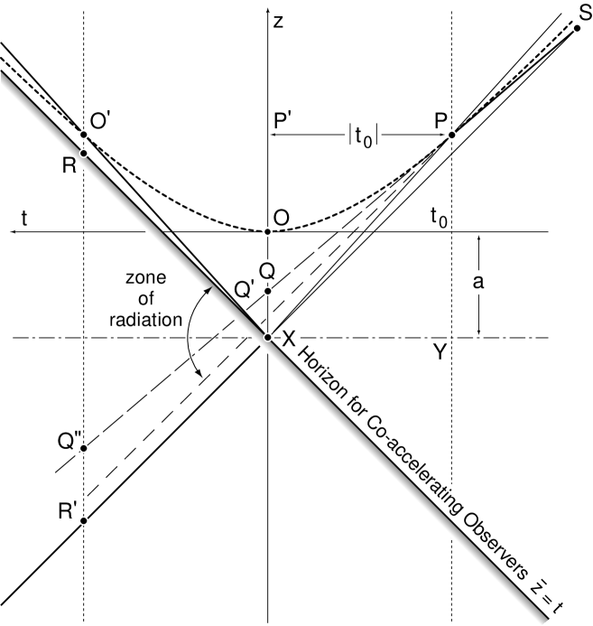
Figure 2a: In this space-time diagram the $z$-axis is upwards and time increases to the left. A charged particle moves uniformly downwards till it reaches $P$ when it is uniformly accelerated upwards coming to momentary rest at $O$ before accelerating up to $O^{\prime}$ and beyond. Had the particle not been accelerated it would have followed $SPQQ^{\prime}Q^{\prime\prime}$. The shaded line $\overline{z}=t$ is the event horizon for an observer accelerating with the charge. $X$ is a distance $c^{2}/\alpha=a$ below $O$; $\alpha$ is the acceleration.

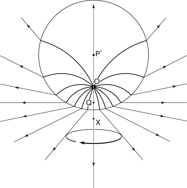
Figure 2b: Shows the lines of electric force in the $xz$ plane that corresponds to the line $OX$ through Figure 2a. The particle is momentarily at rest at $O$ but accelerating upward. The field lines droop under the effective gravity induced by this acceleration but beyond $ct_{0}$ from $P^{\prime}$ there has not been time for the field to be modified from what it would have been had the particle continued on its unaccelerated path to $Q$. The field would then have pointed at the particle so outside a sphere of radius $ct_{0}$ it still points there. There is no magnetic field within that sphere but outside it the field has a magnetic component as though the particle was at $Q$ and still moving downward at a rate that flattens the Coulomb field by a factor 2. The magnetic field is only present in this outer region and lies in rings about the particle’s original motion.

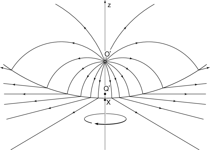
Figure 2c: This corresponds to the slice $O^{\prime}X$ through Figure 2a. The electric field lines are again shown after a Lorentz transformation has reduced the particle at $O^{\prime}$ to rest. Had the particle continued uniformly in a straight line from $P$ it would have been at $Q^{\prime}$, the far field still points there since the message that the particle has been accelerated has not yet come there. In this frame the particle was originally moving even faster so its Coulomb field is flattened by a factor 4.

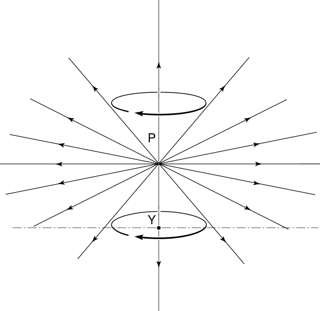
Figure 2d: This corresponds to the vertical slice $PY$ through Figure 2a at time $t_{0}$. The electric field lines are those of a rapidly moving charged particle with the Coulomb field flattened by a factor 2 and the magnetic field of a downward moving charge.

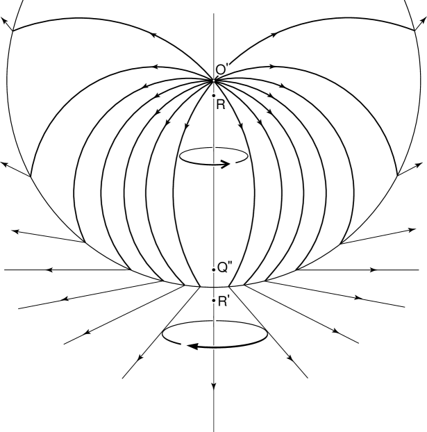
Figure 2e: This corresponds to the vertical slice $O^{\prime}Q^{\prime\prime}$ through Figure 2a. The drooping electric field lines even start reconverging in the region beyond the particle’s event horizon which is the zone where radiation is found. In the near zone the magnetic field has felt the upward motion of the particle so lies in opposing loops to the outer zone where the field still does not appreciate that the particle has ceased its downward motion.

References

- [1] A. Einstein, Viertel jahrsschrift für gerichtliche Medicin und offentliches Sanitat Wesenen 44 (1912).
- [2] A. Einstein, “Letter to Mach in collected papers”, Vol. 5, No. 448, p. 340, Princeton University Press, 1995.
- [3] A. Einstein, “The Meaning of Relativity”, 5th ed., p. 202, Princeton University Press, 1955.
- [4] C.H. Brans, Phys. Rev. 125 (1962), 388.
- [5] H. Thirring, Phys. Z. 19 (1918), 33, ibid. 22 (1921), 29.
- [6] J. Lense and H. Thirring, Phys. Z. 19 (1918), 156.
- [7] D.R. Brill and J.M. Cohen, Phys. Rev. 143 (1966), 1011.
- [8] L. Lindblom and D.R. Brill, Phys. Rev. D 10 (1974), 3151.
- [9] F. Embacher, in “Ernst Mach & the Development of Physics” (V. Prosser and J. Folta, Eds.), Charles University Press, Prague, 1988.
- [10] H. Pfister and K.H. Braun, Class. Quantum Grav. 2 (1985), 909.
- [11] C. Klein, Class. Quantum Grav. 10 (1993), 1619.
- [12] D. Lynden-Bell, J. Katz and J. Bičák, Mon. Not. R. Astr. Soc. 272 (1995), 150. Errata 277 (1995), 1600.
- [13] J. Katz, D. Lynden-Bell and J. Bičák, Class. Quantum Grav. (1998), to be published.
- [14] S.T. Hengge, Diploma Thesis, University of Tubingen (unpublished), 1997.
- [15] H. Farhoosh and R.L. Zimmerman, Phys. Rev. D 21 (1980), 317; see also Gen. Rel. Grav. 12 (1980), 935.
- [16] D. Lynden-Bell, in “Mach’s Principle” (J.B. Barbour and H. Pfister, Eds.), Einstein Studies, Vol. 6, Birkhauser, 1995.
- [17] D. Lynden-Bell and J. Katz, Phys. Rev. D 52 (1995), 7322.
- [18] J. Katz, J. Bičák and D. Lynden-Bell, Phys. Rev. D 55 (1997), 5957.
- [19] T. Fulton and F. Rohrlich, Annals of Phys. 9 (1960), 499.
- [20] N. Rosen, Annals of Phys. 17 (1962), 209.
- [21] M. Born, Ann. Physik 30 (1909), 1.
- [22] G.A. Schott, “Electromagnetic Radiation”, p. 63, Cambridge University Press, 1912. See also Phil. Mag. 29 (1915), 49.
- [23] H. Bondi and T. Gold, Proc. Roy. Soc. (London) A 229 (1955), 416.
- [24] D.G. Boulware, Annals of Phys. 124 (1980), 169.
- [25] J. Bičák and R. Muschall, Wiss Zeits. f. Schiller Univ. Jena Naturwiss 39 (1990), 15.
- [26] J. Bičák, Proc. Roy. Soc. (London) A 371 (1980), 429.
- [27] J.L. Synge, “Relativity the General Theory”, Ch. X, §4, p.367, North Holland, Amsterdam, 1971.
- [28] J.B. Hartle and S.W. Hawking, Commun. Math. Phys. 26 (1972), 87.
- [29] S. Gull, C. Doran and A. Lasenby, in “Clifford (Geometric) Algebras”, (W.E. Baylis, Ed.), p. 95, Birkhäuser, Boston, 1996.
- [30] J. Bičák, Proc. Roy. Soc. (London) A 302 (1968), 201.
- [31] J. Bičák and B.G. Schmidt, Phys. Rev. D 401 (1989), 827.
- [32] J. Bičák, in “Relativistic Gravity and Gravitational Radiation”, Proceedings of the Les Houches School, (J.A. Marck and J.P. Lasota, Eds.), p. 82, Cambridge University Press, 1997.
- [33] S.D. Majumdar, Phys. Rev. 72 (1947), 930.
- [34] A. Papapetrou, Proc. R. Irish Acad. A 51 (1947), 191.
- [35] D. Kramer, H. Stephani, M.A.H. McCallum and E. Herlt, “Exact Solutions of Einstein’s Equations”, Cambridge University Press, 1980.
- [36] A. Das, Proc. Roy. Soc. (London) A 267 (1962), 1.
- [37] W.B. Bonnor and S.B.P. Wickramasuriya, Mon. Not. R. Astr. Soc. 170 (1975), 643.
- [38] W.B. Bonnor, Gen. Rel. Grav. 12 (1980), 453.