GEODESICS IN THE $\gamma$ SPACETIME

Abstract

Circular and radial geodesics are studied in the spacetime described by the $\gamma$ metric. Their behaviour is compared with the spherically symmetric situation, bringing out the sensitivity of the trajectories to deviations from spherical symmetry.

1 Introduction

The influence of small perturbations of a Schwarzschild black hole, on the trajectories of test particles around the source, has atracted the attention of many researchers. These perturbations are usually introduced as additional mass and charge concentrations [1, 2, 3, 4, 5, 6], magnetic fields [7] or gravitational waves [8]. The common results of all these works being, that essentially any perturbation of a Schwarzschild black hole will lead to chaotic orbits.

In this work we want to present another approach to the problem of introducing perturbations to spherical symmetry. This consists in considering an exact solution of Einstein equations continuously linked to the Schwarzschild metric, through one of its parameters. The rationale behind this approach lies on the known [9], though usually overlooked, fact that as the source approaches the horizon, any finite perturbation of the Schwarzschild spacetime, becomes fundamentally different from any Weyl metric, even if the latter is characterized by parameters whose values are arbitrarily close to those corresponding spherical symmetry.

The solution to be considered here is the so called $\gamma$ metric [10, 11], which is also known as the Zipoy-Vorhees metric [12], and belongs to the family of the Weyl solutions [13].

The motivation for this choice may be found in the fact that the $\gamma$ metric corresponds to a solution of the Laplace equation, in cylindrical coordinates, with the same Newtonian source image [14], as the Schwarzschild metric (a rod). In this sense the $\gamma$ metric appears as the natural generalization of the Schwarzschild spacetime to the static axisymmetric case.

We shall find the geodesic equations for test particles in the $\gamma$ metric. Particular attention will be devoted to circular and radial geodesics. The qualitative differences in the dynamics of the test particles as compared to the spherically symmetric case will be illustrated and discussed.

The paper is organized as follows. In the next section the $\gamma$ metric is briefly presented. In section 3 geodesic equations are found and analyzed and in section 4 the gravitational and centrifugal forces are studied. Finally the results are discussed in the last section.

2 The $\gamma$ metric

In cylindrical coordinates, static axisymmetric solutions to the Einstein equations are given by the Weyl metric [13]

$$ds^{2}=e^{2\lambda}dt^{2}-e^{-2\lambda}[e^{2\mu}(d\rho^{2}+dz^{2})+\rho^{2}d\phi^{2}],$$ (1)

with

$$\lambda_{,\rho\rho}+\rho^{-1}\lambda_{,\rho}+\lambda_{,zz}=0,$$ (2)

and

$$\mu_{,\rho}=\rho(\lambda^{2}_{,\rho}-\lambda^{2}_{,z}),\qquad\mu_{,z}=2\rho\lambda_{,\rho}\lambda_{,z}.$$ (3)

Observe that (2) is just the Laplace equation for $\lambda$ in the Euclidean space.

The $\gamma$ metric is defined by [10]

$$e^{2\lambda} = \left(\frac{R_{1}+R_{2}-2m}{R_{1}+R_{2}+2m}\right)^{\gamma},$$ (4)

$$e^{2\mu} = \left[\frac{(R_{1}+R_{2}+2m)(R_{1}+R_{2}-2m)}{4R_{1}R_{2}}\right]^{\gamma^{2}},$$ (5)

where

$$R_{1}^{2}=\rho^{2}+(z-m)^{2},\qquad R_{2}^{2}=\rho^{2}+(z+m)^{2}.$$ (6)

It is worth noticing that $\lambda$, as given by (4), corresponds to the Newtonian potential of a line segment of mass density $\gamma/2$ and length $2m$, symmetrically distributed along the $z$ axis. The particular case $\gamma=1$, corresponds to the Schwarzschild metric.

It will be useful to work in Erez-Rosen coordinates [12], given by

$$\rho^{2}=(r^{2}-2mr)\sin^{2}\theta,\qquad z=(r-m)\cos\theta,$$ (7)

which yields the line element (1) with (4,5) as [10]

$$ds^{2}=Fdt^{2}-F^{-1}[Gdr^{2}+Hd\theta^{2}+(r^{2}-2mr)\sin^{2}\theta d\phi^{2}],$$ (8)

where

$$F = \left(1-\frac{2m}{r}\right)^{\gamma},$$ (9)

$$G = \left(\frac{r^{2}-2mr}{r^{2}-2mr+m^{2}\sin^{2}\theta}\right)^{\gamma^{2}-1},$$ (10)

$$H = \frac{(r^{2}-2mr)^{\gamma^{2}}}{(r^{2}-2mr+m^{2}\sin^{2}\theta)^{\gamma^{2}-1}}.$$ (11)

Now it is easy to check that $\gamma=1$ corresponds to the Schwarzschild metric.

The total mass $M$ of the source is [10, 11]

$$M=\gamma m,$$ (12)

and the quadrupole moment $Q$ is given by

$$Q=\frac{\gamma}{3}(1-\gamma^{2})M^{3}.$$ (13)

From (13) we have that $\gamma>1(\gamma<1)$ corresponds to the oblate (prolate) spheroid.

3 The geodesics

The equations governing the geodesics can be derived from the Lagrangian

$$2{\cal L}=g_{\alpha\beta}\dot{x}^{\alpha}\dot{x}^{\beta},$$ (14)

where the dot denotes differentiation with respect to an affine parameter $s$ , which for timelike geodesics coincides with the proper time. Then, from the Euler-Lagrange equations,

$$\frac{d}{ds}\left(\frac{\partial{\cal L}}{\partial\dot{x}^{\alpha}}\right)-\frac{\partial{\cal L}}{\partial x^{\alpha}}=0,$$ (15)

it follows, for the metric (8),

$$\ddot{t}+\gamma\dot{t}\dot{r}\nu^{\prime}=0,$$ (16)

$$-2\ddot{r}\frac{e^{-\gamma\nu}}{A^{\gamma^{2}-1}}+\dot{r}^{2}\left[\gamma\frac{e^{-\gamma\nu}\nu^{\prime}}{A^{\gamma^{2}-1}}+(1-\gamma^{2})m^{2}\>\frac{e^{-(1+\gamma)\nu}}{r^{2}A^{\gamma^{2}}}\left(\frac{2}{r}+\nu^{\prime}\right)\sin^{2}\theta\right]$$

$$-4\dot{r}\dot{\theta}(1-\gamma^{2})m^{2}\>\frac{e^{-(1+\gamma)\nu}}{r^{2}A^{\gamma^{2}}}\sin\theta\cos\theta-\dot{t}^{2}\gamma\nu^{\prime}e^{\gamma\nu}$$

$$+\dot{\theta}^{2}\left\{\frac{r^{2}e^{(1-\gamma)\nu}}{A^{\gamma^{2}-1}}\left[\frac{2}{r}+(1-\gamma)\nu^{\prime}\right]+(1-\gamma^{2})m^{2}\>\frac{e^{-\gamma\nu}}{A^{\gamma^{2}}}\left(\frac{2}{r}+\nu^{\prime}\right)\sin^{2}\theta\right\}$$

$$+\dot{\phi}^{2}r^{2}e^{(1-\gamma)\nu}\left[\frac{2}{r}+(1-\gamma)\nu^{\prime}\right]\sin^{2}\theta=0,$$ (17)

$$-\ddot{\theta}\frac{r^{2}e^{(1-\gamma)\nu}}{A^{\gamma^{2}-1}}-\dot{\theta}^{2}(1-\gamma^{2})m^{2}\>\frac{e^{-\gamma\nu}}{A^{\gamma^{2}}}\sin\theta\cos\theta$$

$$+\dot{\theta}\dot{r}\left\{-\frac{r^{2}e^{(1-\gamma)\nu}}{A^{\gamma^{2}-1}}\left[\frac{2}{r}+(1-\gamma)\nu^{\prime}\right]+(1-\gamma^{2})m^{2}\>\frac{e^{-\gamma\nu}}{A^{\gamma^{2}}}\left(\frac{2}{r}+\nu^{\prime}\right)\sin^{2}\theta\right\}$$

$$+\dot{r}^{2}(1-\gamma^{2})m^{2}\>\frac{e^{-(1+\gamma)\nu}}{r^{2}A^{\gamma^{2}}}\sin\theta\cos\theta+\dot{\phi}^{2}r^{2}e^{(1-\gamma)\nu}\sin\theta\cos\theta=0,$$ (18)

$$\left\{\ddot{\phi}+\dot{\phi}\dot{r}\left[\frac{2}{r}+(1-\gamma)\nu^{\prime}\right]+2\dot{\phi}\dot{\theta}\cot\theta\right\}e^{(1-\gamma)\nu}\sin^{2}\theta=0,$$ (19)

with

$$e^{\nu}\equiv 1-\frac{2m}{r},\qquad A\equiv 1+\frac{m^{2}e^{-\nu}\sin^{2}\theta}{r^{2}},$$ (20)

and prime denotes differentiation with respect to $r$.It is a simple matter to check that if $\gamma=1$ we recover the geodesic equations of the Schwarzschild spacetime.

Let us first consider circular geodesics. From (16-19) we obtain using $\dot{r}=\dot{\theta}=0$,

$$\ddot{t}=\ddot{\phi} = 0,$$ (21)

$$\gamma\dot{t}^{2}e^{\gamma\nu}\nu^{\prime} = \dot{\phi}^{2}r^{2}e^{(1-\gamma)\nu}\left[\frac{2}{r}+(1-\gamma)\nu^{\prime}\right]\sin^{2}\theta,$$ (22)

$$2\dot{\phi}^{2}r^{2}e^{(1-\gamma)\nu}\sin\theta\cos\theta = 0.$$ (23)

Then from the definiton of the angular velocity $\omega$ of a test particle along circular geodesics

$$\omega=\frac{\dot{\phi}}{\dot{t}},$$ (24)

we obtain, using (22),

$$\omega^{2}=\frac{\gamma m}{[r-(1+\gamma)m]r^{2}\sin^{2}\theta}\left(1-\frac{2m}{r}\right)^{2\gamma-1}.$$ (25)

First of all, we observe that, as it follows from (23), circular geodesics out of the equatorial plane $\theta=\pi/2$, are now possible, if only $\gamma<1$ and $r=2m$. This kind of trajectories do not exist in Schwarzschild spacetime ($\gamma=1$). From (25) it also follows that physically meaningful values of $\omega$ at $r=2m$, exist only for $\gamma=1/2$. Therefore circular geodesics for $\theta\neq\pi/2$ can ocur if only $\gamma=1/2$ and $r=2m$, with angular velocity

$$\omega^{2}=\frac{1}{4m^{2}\sin^{2}\theta}.$$ (26)

Circular geodesics outside the equatorial plane also exist in the Kerr metric [15]. These kind of orbits implies the presence of repulsive forces whose nature is still not well understood [16, 17]. However it should be stressed that since $r=2m$ represents a physical singularity in the $\gamma$ metric, these orbits are deprived of physical meaning. In the weak field limit one obtains from (25), for $\theta=\pi/2$, up to the first order in $m/r$,

$$\omega^{2}\approx\frac{\gamma m}{r^{3}}\left[1+(1-\gamma)\frac{3m}{r}\right]+O\left(\frac{m}{r}\right)^{2}.$$ (27)

If $\gamma=1$, we recover the well known Kepler law, which is also valid, if $\gamma=1$, without any approximation.

If $\gamma\neq 1$ the second term within the brackets, in (27), gives the correction due to the quadrupole moments of the source. In troducing the dimensionless variable $x\equiv 2m/r$, we can rewrite (25), for $\theta=\pi/2$,

$$\tilde{\omega}^{2}\equiv m^{2}\omega^{2}=\frac{\gamma(1-x)^{2\gamma-1}x^{3}}{4[(1-\gamma)x+2(1-x)]}.$$ (28)

Figure 1 shows the behaviour of $\tilde{\omega}^{2}$ as a function of $x$ for different values of $\gamma$, including $\gamma=1$.

The bifurcation between the $\gamma=1$ and $\gamma\neq 1$ cases, for values of $x$ close to one, clearly illustrates the sensitivity of the system under perturbations of $\gamma$ in the neighborhood of $\gamma=1$.

For comparative purposes it will be useful to find an expression for the tangential velocity $W^{\mu}$ of the test particle along the circular geodesic. From [18], we have

$$W^{\alpha}=\frac{V^{\alpha}}{\sqrt{g_{00}}dx^{0}},$$ (29)

with

$$V^{\alpha}=(0,dx^{1},dx^{2},dx^{3}),$$ (30)

and we obtain from (8) for $\theta=\pi/2$,

$$W^{2}\equiv W_{\alpha}W^{\alpha}=\left(1-\frac{2m}{r}\right)^{1-2\gamma}\omega^{2}r^{2}=\frac{\gamma m}{r-(1+\gamma)m},$$ (31)

where $\omega^{2}$ is given by (25). In the weak field limit, $m/r\ll 1$, the classical expression, $W=\omega r$ is recovered. Figure 2 shows $W^{2}$ as a function of $x$ for different values of $\gamma$. Furthermore, we see from (31), that null circular geodesics appear when $r=(1+2\gamma)m$. Since the physical singularity lies for $r=2m$ then null circular geodesics can only exist for $\gamma>1/2$, otherwise, for $\gamma<1/2$, they do not exist.

The Levi-Civita metric, which represents the field of an infinite line mass of constant energy density $\sigma$, can be obtained as a limiting case from the $\gamma$ metric by taking $m\rightarrow\infty$ and associating $\gamma=2\sigma$ [19]. Next we see, in the equatorial plane, how the angular velocity $\omega$ and the tangential velocity $W$ of the circular geodesics, respectively given by (25) and (31), behave for big values of $m$.

Rewriting (25) in terms of the coordinates given by (7), with $\theta=\pi/2$, we obtain

$$\omega^{2}=\frac{\gamma m(\sqrt{m^{2}+\rho^{2}}-m)^{2\gamma-1}}{(\sqrt{m^{2}+\rho^{2}}-\gamma m)(m+\sqrt{m^{2}+\rho^{2}})^{2\gamma+1}}.$$ (32)

Expanding in series (32) for big values of $m$ and keeping only the term in its lowest order of $\rho/m$, we obtain

$$\omega^{2}\approx\frac{2\sigma}{1-2\sigma}(4m^{2})^{-4\sigma}\rho^{2(4\sigma-1)},$$ (33)

where we have substituted $\gamma=2\sigma$. The expression (33) is the same as for the Levi-Civita metric obtained in [17] provided the topological defect $a$, as given in [17], is associated in (33) as $a=(4m)^{-2\sigma}$. In [19] it is proved that the limiting case of Levi-Civita spacetime from the $\gamma$ spacetime produces an infinite topological defect.

Now rewriting (31) in terms of the coordinates given by (7), we have

$$W^{2}=\frac{\gamma m}{\sqrt{m^{2}+\rho^{2}}-\gamma m}.$$ (34)

Expanding (34) in series for big values of $m$ up to the second order of $\rho/m$, we obtain

$$W^{2}\approx\frac{2\sigma}{1-2\sigma}-\frac{2\sigma}{2(1-2\sigma)^{2}}\left(\frac{\rho}{m}\right)^{2}+O\left(\frac{\rho}{m}\right)^{4},$$ (35)

where we have substituted $\gamma=2\sigma$. From (35) we have that, for a given $\gamma$ and a fixed radius $\rho$, decreasing the length $2m$ of the line segment of mass decreases the tangential speed $W$ of the circular geodesics.When $m\rightarrow\infty$ we have that the tangential velocity (34) is the same as the one obtained for the Levi-Civita metric [17], being

$$\lim_{m\rightarrow\infty}W^{2}=\frac{\gamma}{1-\gamma}=\frac{2\sigma}{1-2\sigma}.$$ (36)

Observe that (36) sets a constraint on possible values of $\sigma$ to avoid values of $W$ larger than 1, i.e. the velocity of light. This is in contrast with the situation in the $\gamma$ metric (34), where such constraint $W\leq 1$ involves $\gamma$ and the radial coordinate $\rho$ of the orbit.

Let us now consider radial geodesics. From (8), in the $\theta=\pi/2$ plane, it follows

$$1=\dot{t}^{2}\left(1-\frac{2m}{r}\right)^{\gamma}-\dot{r}^{2}\left(1-\frac{2m}{r}\right)^{-\gamma}\left(\frac{r^{2}-2rmr}{r^{2}-2mr+m^{2}}\right)^{\gamma^{2}-1}$$

$$-\dot{\phi}^{2}\left(1-\frac{2m}{r}\right)^{1-\gamma}r^{2}.$$ (37)

Next, it follows from (15),

$$\frac{\partial{\cal L}}{\partial\dot{t}}=\mbox{constant}=E = \dot{t}\left(1-\frac{2m}{r}\right)^{\gamma},$$ (38)

$$\frac{\partial{\cal L}}{\partial\dot{\phi}}=\mbox{constant}=L = -\dot{\phi}\left(1-\frac{2m}{r}\right)^{1-\gamma}r^{2},$$ (39)

where $E$ and $L$ represent, respectively, the total energy and the angular momentum of the test particle. Then using (38,39) in (37), we obtain

$$\dot{r}^{2}=\left(1-\frac{2m}{r}\right)^{\gamma^{2}-1}(E^{2}-V^{2}),$$ (40)

where $V(x)$, which can be associated to the potential energy of the test particle, is given by

$$V^{2}\equiv\left(1-\frac{2m}{r}\right)^{\gamma}\left[\frac{m^{2}\tilde{L}^{2}}{r^{2}}\left(1-\frac{2m}{r}\right)^{\gamma-1}+1\right],$$ (41)

with

$$\tilde{L}^{2}\equiv\frac{L^{2}}{m^{2}},$$ (42)

or, in terms of $x$ (41) becomes

$$V^{2}=\left(1-\frac{2}{x}\right)^{\gamma}\left[\frac{\tilde{L}^{2}}{x^{2}}\left(1-\frac{2}{x}\right)^{\gamma-1}+1\right].$$ (43)

Figure 3 shows $V$ for different values of $\gamma$ and $\tilde{L}^{2}=55$. For indicated values of the total energy $E$, there exist unstable circular orbits, which illustrate the sensitivity to small perturbations.

4 Gravitational and centrifugal forces

The study of the gravitational and centrifugal forces follows the same treatment as in [20]. The four velocity of a particle moving on a circular orbit in the equatorial plane $\theta=\pi/2$ of the $\gamma$ spacetime (8) can be expressed as

$$v^{\alpha}=(\delta^{\alpha}_{t}+\Omega\delta^{\alpha}_{\phi})\Gamma,$$ (44)

where $\Omega$ is a parameter and, since $v_{\alpha}v^{\alpha}=1$, $\Gamma$ is given by

$$\Gamma^{2}=\frac{F}{F^{2}-\Omega^{2}r(r-2m)}.$$ (45)

Assuming uniform motion, $\Omega=$constant, the acceleration $a^{\alpha}$ of the particle,

$$a^{\alpha}=v^{\beta}v^{\alpha}_{;\beta},$$ (46)

using (8,44,45) is

$$a^{\alpha}=\delta^{\alpha}_{r}\frac{r^{1-\gamma-\gamma^{2}}(r-2m)^{\gamma(1-\gamma)}(r-m)^{2(\gamma^{2}-1)}}{r^{-2\gamma}(r-2m)^{2\gamma-1}-\Omega^{2}r}$$

$$\times\left\{\frac{\gamma m}{r^{2}}\left(1-\frac{2m}{r}\right)^{2\gamma-1}-\Omega^{2}[r-(1+\gamma)m]\right\}.$$ (47)

If $\gamma=1$, then (47) reduces to the Schwarzschild spacetime result [20],

$$a^{\alpha}=\delta^{\alpha}_{r}\frac{1}{r}\left(1-\frac{2m}{r}\right)\frac{m-\Omega^{2}r^{3}}{r-2m-\Omega^{2}r^{3}}.$$ (48)

The acceleration $a^{\alpha}$ can be split into its gravitational component $g^{\alpha}$, when $\Omega=0$, and its centrifugal component $c^{\alpha}$, as

$$-a^{\alpha}=g^{\alpha}+c^{\alpha},$$ (49)

and so we have from (47),

$$g^{\alpha} = -\delta^{\alpha}_{r}\frac{\gamma m}{r^{2}}\left(1-\frac{2m}{r}\right)^{\gamma(1-\gamma)}\left(1-\frac{m}{r}\right)^{2(\gamma^{2}-1)},$$ (50)

$$c^{\alpha} = \delta^{\alpha}_{r}\Omega^{2}r[r-(1+2\gamma)m]\frac{(r-2m)^{\gamma(1-\gamma)}(r-m)^{2(\gamma^{2}-1)}}{r^{\gamma(\gamma-1)}(r-2m)^{2\gamma-1}-\Omega^{2}r^{\gamma^{2}+\gamma+1}}.$$ (51)

When the gravitational acceleration is balanced by the centrifugal acceleration, which means $a^{\alpha}=0$, then we have $\Omega=\omega$, as it can be checked from (25). The gravitational acceleration $a^{\alpha}$ always points inwards, being $g^{\alpha}<0$. The centrifugal acceleration $c^{\alpha}$ for values of $r>(1+2\gamma)m$ is always positive, while for $r<(1+2\gamma)m$ it becomes negative. Since $r=2m$ is the physical singularity only $1/2<\gamma$ allows negative values for $c^{\alpha}$, while $1/2>\gamma$ makes always $c^{\alpha}$ positive.

5 Conclusions

We have considered deviations from spherical symmetry by considering exact solutions of the Weyl family, instead of perturbing the Schwarzschild metric. As it should be expected from the Israel theorem [21], these approaches differ qualitatively as the orbit of the test particle gets close to the horizon. Though it was not our purpose here to describe the chaotic behaviour of the trajectories, it should be clear that such behaviour is the expression of the sensitivity to small changes of $\gamma$. This sensitivity in turn, appears sistematically in the cinematics of the particles, for orbits close to $2m$, as illustrated by figures 1–3.

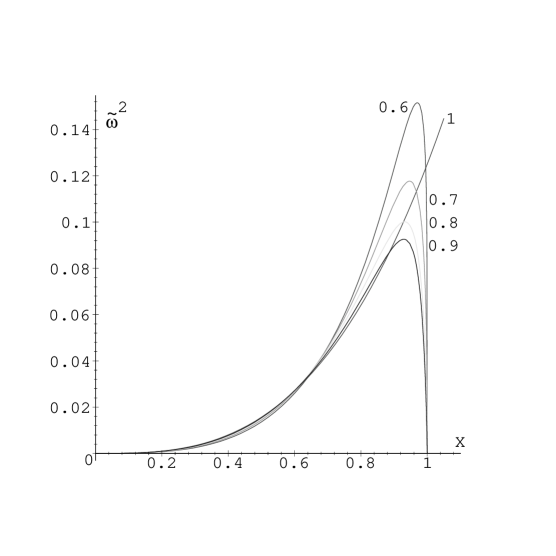
Figure 1: $\tilde{\omega}^{2}$ as function of $x$ for the five values of $\gamma$ indicated.

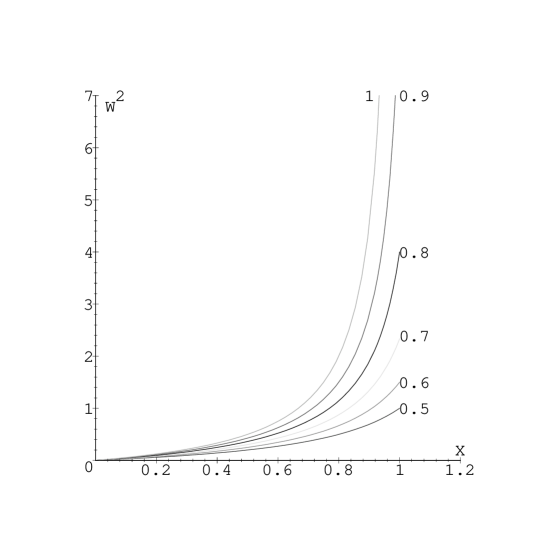
Figure 2: $W^{2}$ as function of $x$ for six different values of $\gamma$.

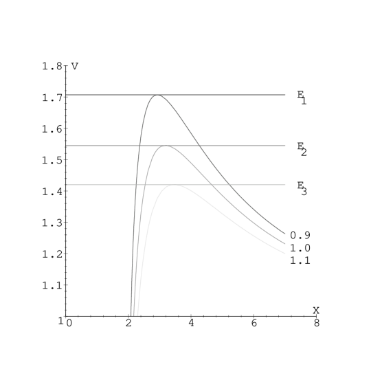
Figure 3: $V$ as function of $x$ for three different values of $\gamma$. For the three values of $E$, there are three different unstable circular orbits.

References

- [1] Chandrasekhar S Proc. R. Soc. London A 421 227 (1989)
- [2] Contopoulos G Proc. R. Soc. London A 431 183 (1990); 435 551 (1991)
- [3] Moeckel R Commun. Math. Phys. 150 415 (1992)
- [4] Dettmann C P, Frankel N E and Cornish N J Phys. Rev. D 50 R618 (1994); Fractals 3 161 (1995)
- [5] Vieira W M and Letelier P S Phys. Rev. Lett. 76 1409 (1996)
- [6] Cornish N J and Frankel N E Phys. Rev. D 56 1903 (1997)
- [7] Karas V and Vokrouhlicky Gen. Rel. Grav. 24 729 (1992)
- [8] Bombelli L and Calzetta E Class. Quantum Grav. 9 2573 1992)
- [9] Winicour J, Janis A and Newman E Phys. Rev. 176 1507 (1968); Janis A, Newman E and Winicour J Phys. Rev. Lett. 20 878 (1968); Cooperstock F I and Junevicus G J G Il Nuovo Cimento 16B 387 (1973)
- [10] Esposito F and Witten L Phys. Lett. 58B 357 (1975)
- [11] Virbahdra K S Directional naked singularities in General Relativity preprint gr-gc/9606004
- [12] Bach R and Weyl H Math. Z. 13 134 (1920); Darmois G Les quations de la gravitation Einsteinienne (Gauthier-Villars, Paris, 1927) p.36; Erez G and Rosen N Bull. Res. Council Israel 8F 47 (1959); Zipoy D M J. Math. Phys. 7 1137 (1966); Gautreau R and Anderson J L Phys. Lett. A 25 291 (1967); Cooperstock F and Junevicus G Int. J. Theor. Phys. 9 59 (1968); Vorhees B Phys. Rev. D 2 2119 (1970)
- [13] Weyl H Ann. Phys. 54 117 (1918); 59 185 (1919); Levi-Civita T Atti. Accad. Naz. Lincei Rend. Classe Sci. Fis. Mat. e Nat. 28 101 (1919); Synge J L Relativity: the general theory (North-Holland Publ. Co., Amsterdam, 1960)
- [14] Bonnor W B Proceedings of the 3rd Canadian Conference on General Relativity and Relativistic Astrophysics eds. Coley A, Cooperstock F I and Tupper B (World Scientific Publishing Co., Singapore, 1990) p. 216
- [15] Bonnor W B J. Phys. A [10 1673 (1977)
- [16] Schücking E L Atti del Convegno sulla Cosmologia (G Barbèra Editore, Florence, 1966)
- [17] Herrera L and Santos N O J. Math. Phys. 39 3817 (1998)
- [18] Anderson J L Principles of Relativity (Academic Press, New York, 1967) Sec. 10.6(a)
- [19] Herrera L, Paiva M Paiva and Santos N O The Levi-Civita spacetime as a limiting case of the spacetime preprint (1998) gr-qc/9810079
- [20] Sonego S and Massar M Mon. Not. R. Astron. Soc. 281 659 (1996)
- [21] Israel W Phys. Rev. 164 1776 (1967)